Approximation method for the sewer drainage effect for urban flood modeling in areas without drainage-pipe data

Introduction: The underground drainage-pipe network is one of the vital components of a modern city, and it plays an important role in preventing or mitigating urban flooding. Thus, pipe network data are necessary for simulation of the entire urban rainfall–runoff process. However, pipe network data are sparse or unavailable in most urban areas.

Methods: To solve this problem, we developed a novel approximation method that can be used calculate the drainage capacity of the pipe system. This method is named the road-drainage method, and it works under the assumption that the pipe network functions by subtracting the corresponding mass from the water conservation equation only from areas of road. The mass is determined from weir flow formulas together with the road properties and correction for this mass is applied to the rainfall source term.

Results: Two test cases were used to compare the performance of the new method with an existing method, under which mass is subtracted from the entire area during the rainfall–runoff process. The results showed that the new method considerably improves the accuracy of simulated peak volume, with an improvement of 2.62%–58.75% compared with the existing method across various scenarios. Moreover, the proposed new method reduces the time shift of the rise and peak of surface inundation by 10–45 min in various scenarios, which reflects a more realistic model of the rainfall–runoff process.

Discussion: These results demonstrate that the proposed new method can represent the drainage capability more accurately and is more consistent with reality. The road-drainage method has promising potential for application in urban flood simulation in areas without drainage system data and for the support of large-scale urban hydrologic modeling.

1 Introduction

Urban floods that severely affect urban development, caused by climate change and rapid urbanization, have become one of the more serious urban hazards (Ali et al., 2011; Zhang and Pan, 2014; Lashford et al., 2019; Kratt et al., 2020). The increasing frequency and intensity of extreme rainfall events have inevitably caused extra surface runoff that exceeds designed drainage capacity (Jang et al., 2018; Ilderomi et al., 2022; Jia et al., 2022; Kuriqi and Hysa, 2022), which causes further urban floods. A better understanding of the causes of flooding is crucial for flood risk management (Debarati et al., 2016; Tariq et al., 2021; Avand et al., 2022). As an essential part of drainage infrastructure, the pipeline is often complex and staggered underground, which makes it more challenging to evaluate drainage capacity using a numerical model (Jang et al., 2018).

In recent years, with increasing computational performance, the availability of high-resolution data, and the demand for detailed information on flood location and drainage efficiency, one-dimensional (1D) and two-dimensional (2D) coupled models are commonly used for urban flood and inundation simulation (Bladé et al., 2012; Li et al., 2022). Most such 1D and 2D coupled models have been developed by coupling with the Storm Water Management Model (SWMM) to emulate the full rainfall–runoff and drainage process (Adeogun et al., 2015; Wu et al., 2017; Martinez et al., 2018). The same methodology is also used in some commercial software, for example, XP-SWMM (SOLUTIONS.X.P, 2013) and MIKE SWMM (I., 2014). In addition, many researchers have developed other coupled models for urban flooding. Bladé et al. (2012) used a fully conservative 1D and 2D coupled model based on finite volumes to emulate a characterization of the fluid dynamics of a river–reservoir system in the River Ebro in Spain. Fan et al. (2017) introduced and tested a coupled model based on the implicit technique in a real-world urban catchment. Chang et al. (2015) developed a new coupled model for urban flood modeling that simulates flow interactions between sewers and the surface. Jang et al. (2018) used a coupled flood model based on diffusion waves to investigate the impact of inlet modeling on drainage efficiency.

Nevertheless, these models are subject to several limitations, mainly arising when they are applied in an area without drainage-pipe data (Li et al., 2020; Hou et al., 2021). In most urban areas, drainage-pipe networks built decades ago were either lost or barely documented when constructed, which has consequently resulted in a lack of drainage system data. Even if there is a drainage network layout drawing, it is usually inconsistent with the actual drainage system due to adjustments made during construction. Furthermore, onsite measurement of the layout of the drainage network is both expensive and difficult (Tscheikner-Gratl et al., 2019; Kratt et al., 2020). Under such circumstances, to cope with this problem, several approximation methods combined with the 2D model have been considered as alternative approaches for the simulation of urban rainfall–runoff processes. Some of the most common approximation methods used to calculate drainage effects on pipe networks include the discounted rainfall rate method and fixed infiltration rate method. The United Kingdom Environment Agency (AGENCY, 2013) reduced its design rainfall to account for the effect of drainage capacity. Hou et al. (2018) used stable infiltration, with a value of 10.47 mm/h across the entire study area, to reflect urban drainage capacity when simulating rainfall–runoff inundation processes. Wang et al. (2018) used two approaches—rainfall reduction and constant infiltration at 5 mm/h ∼ 20 mm/h—to represent the urban drainage effect. These studies show that the constant infiltration method is better than the rainfall reduction method for representing drainage capacity, which could be explained by the fact that the constant infiltration method provides a more accurate description of the flood recession process than the constant rain reduction method.

However, all the aforementioned methods assume that the drainage effect is at work over the entire study area, which is inconsistent with the actual rainfall–runoff process, resulting in a large simulation error and difficulty in ensuring calculation accuracy in the actual process. Several studies have shown that most of the drainage pipe network is laid along roads, and the real runoff process should be conceptualized as follows: after rainfall occurs, water will first flow to the road area after generation and confluence and will then be discharged through the rainwater pipe network. For example, Li et al. (2020) proposed a method for approximate computation of inlet drainage, in which the inlet or gully was assumed to be a drainage area, and the weir equation was used to calculate the water discharged into the drainage system from the surface. However, it is difficult to extract the location of the gully, especially in a large urban area. Inspired by the valuable findings of the aforementioned research, the main purpose of this study was to propose an effective method for approximate calculation of the drainage effect that is more in line with the actual physical process. Specifically, a new method (named the road-drainage method) is proposed that incorporates the role of the drainage effect by subtracting mass in the balance equation only from the road area. The rainfall–runoff drainage processes were simulated using a 2D urban hydrodynamic flood model with the proposed road-drainage method incorporated. Moreover, the simulation results from a coupled model consisting of a 2D surface model and a 1D pipe network model were used as a benchmark to evaluate the performance of the new and existing methods.

The specific objectives of this study were: 1) to introduce the governing equations and numerical schemes of the numerical models used in the study, including the 2D surface flow model, 1D sewer flow model, and 1D–2D coupled calculation method; 2) to propose a novel method for approximate computation of drainage capacity in urban flood modeling, which can be used in certain urban areas without drainage data; 3) to evaluate the simulation performance of the proposed method for surface inundation and time shift; and finally, 4) to provide practical recommendations for flood simulation in urban areas without drainage-pipe data. We believe that this research can provide valuable information for modelers and further improve the simulation accuracy of urban rainfall–runoff processes in cases of missing pipe network data. In addition, the approximation method can also be used to study the process of surface runoff and inundation processes for research areas with large amounts of pipe network data to reduce the complexity of the model and improve the efficiency of simulation calculations (Hou et al., 2021). The paper is organized as follows: the numerical model and methods of approximate computation are briefly introduced in Section 2; Section 3 provides brief information on the case study; the results are presented in Section 4; and the discussion and conclusions are given in Section 5.

2 Numerical model and approximation method

Soil infiltration, evaporation, surface runoff, and sewer discharge are the four components of the rainfall–runoff process (Li et al., 2020). The volume of water discharged into the sewer system can be estimated by mass subtraction from a water balance perspective. This work introduces two approximation methods for this problem, namely an existing method and a new method. Under the concept of the existing method, the corresponding water volume of the entire area is subtracted to reflect the drainage effect of the sewer pipe, while in the new method, the capacity of the drainage pipes is represented by subtracting the mass from the road area only. Both these methods neglect the hydrodynamic processes of the sewer flow, which means that only mass balance in the 2D surface model is taken into consideration. The modification of the rainfall source term represents the drainage effect.

The existing method reduces water mass in the process of runoff generation, while the new method deducts the water quantity after the rainwater flows to the road, which is much closer to the actual case (Li et al., 2020; Klipalo et al., 2022). In this study, a hydrodynamics-based urban flood model was adopted as a standard for comparison with the two methods. Thus, three methods were applied in this work to calculate the capacity of drainage pipes: the new method, the existing method, and the coupled model method. The methodology of each of the three methods is described in detail below.

2.1 Numerical model

The rainfall–runoff and inundation model based on hydrodynamics couples the 2D surface flow model and 1D SWMM, which couples underground drainage systems and surface flows. The surface flow model with rainfall generation and overland flow processes solves the 2D shallow water equations (SWEs) using the dynamic wave method. The SWMM is used to simulate the hydrodynamic flow process of a pipe or channel. The 1D–2D coupled model was developed and verified in detail by Li et al. (2022). The governing equations and numerical methods for the different processes are described in detail below.

2.1.1 Governing equations for the surface flow model

The surface flow model solves the SWEs, which are derived from the Navier–Stokes equations, and assumes hydrostatic pressure distribution. If the kinematic and turbulent viscosity terms, wind stresses, and Coriolis effects are neglected, a conservation law of two-dimensional non-linear SWEs can be written in vector form as follows (Liang and Marche, 2009; Xia et al., 2017):

$\frac{\partial \mathit{q}}{\partial \mathit{t}}+\frac{\partial \mathit{f}}{\partial \mathit{x}}+\frac{\partial \mathit{g}}{\partial \mathit{y}}=\mathit{S},(1)$

$\mathit{q}=\left[\begin{array}{l}h\\ q_x\\ q_y\end{array}\right],\mathit{f}=\left[\begin{array}{c}uh\\ {uq}_x+{gh}^{\mathit{2}}/\mathit{2}\\ {uq}_y\end{array}\right],\mathit{g}=\left[\begin{array}{c}vh\\ {vq}_x\\ {vq}_y+{gh}^{\mathit{2}}/\mathit{2}\end{array}\right],\mathit{S}=\left[\begin{array}{l}R\\ -gh\partial z_b/\partial x-C_{f}u\sqrt{u^{\mathit{2}}+v^{\mathit{2}}}\\ -gh\partial z_b/\partial y-C_{f}v\sqrt{u^{\mathit{2}}+v^{\mathit{2}}}\end{array}\right],(2)$

where x and y are the Cartesian coordinates; t represents time; q denotes the vector of conserved flow variables consisting of h and uh and vh, which are the water depth and unit-width discharges in the x and y directions; f and g are the flux vectors in the x and ydirections, respectively; g is gravity; S is the source vector, which can be further subdivided into net rain terms R, friction terms S_f, and slope terms S_b; and C_f depends on the Manning coefficient and can be expressed as C_f = gn²/h^1/3, where n is the Manning coefficient.

R represents the rainfall term, including evaporation, infiltration, rainfall, and water exchange between the surface model and sewer model. However, the surface flow model ignores evaporation and interception; therefore, R in the surface flow model can be written as in Eq. 3 (Li et al., 2020).

$R=i-f_c.(3)$

Here, $i$ is the rainfall and $f_c$ represents infiltration.

2.1.2 Governing equations for the 1D sewer flow model

The SWMM (Rossman, 2009), developed by the United States Environmental Protection Agency (USEPA), is one of the most widely used dynamic rainfall–runoff simulation models for simulating runoff from primarily urban areas. The SWMM consists of two major components, the runoff component and the routing component. In this study, only the routing component was integrated into the coupled model in the form of the 1D sewer flow module. Moreover, dynamic wave analysis solves the complete form of the Saint-Venant flow equations and therefore produces the most theoretically accurate results. It can account for channel storage, backwater effects, entrance/exit losses, culvert flow, flow reversal, and pressurized flow. Thus, dynamic wave theory was selected to analyze the routing process in the sewer system. In the transport compartment, the SWMM solves the Saint-Venant equation using the implicit finite difference method and successive approximation. The Saint-Venant equation consists of mass conservation and momentum conservation equations, and can be expressed as follows (Rossman, 2009):

$\frac{\partial A}{\partial t}+\frac{\partial Q}{\partial x}=0,(4)$

$\frac{\partial Q}{\partial t}+\frac{\partial \left(Q^2/A\right)}{\partial x}+gA\frac{\partial H}{\partial x}+gA{S}_{f1D}=0,(5)$

where $A$ is the flow cross-sectional area, $t$ denotes time, $Q$ is the flow rate, $g$ is the acceleration of gravity, $H$ is the hydraulic head of water in the conduit (Z + Y), Z is the conduit invert elevation, Y is the conduit water depth, and $S_{f1D}$ is the friction slope (head loss per unit length).

2.1.3 Coupling between the 2D and 1D models

The rainfall–runoff drainage processes in the sewer networks and surfaces were simulated by coupling the 2D surface flow model and the SWMM model. The two models were connected through appropriate linkages to exchange water level and flow, after both had been executed individually to a suitable time. Rainfall was simulated in the 2D surface model; this form is more in line with the actual process (Chen et al., 2018).

Between the sewer system and the surface, only vertical exchange occurs in most cases. Water enters the drainage pipe system at the inlet when it flows through the inlets. When the water depth in an inlet exceeds the elevation of the surface, flooding from the sewer pipes to the surface occurs. In this work, the water exchange between the sewer and surface was coupled through the inlet (hereinafter, this approach is referred to as the coupled model). For the sewer pipe system simulation, only the vertical linkage was considered.

The model calculates inflow using the weir equation or the orifice equation (Eq. 6), considering surface water flow to the sewer system (Figure 1) (Chen et al., 2007; Chen et al., 2018).

$Q_{in}=\left\{\begin{array}{l}{c}_w{C}_i{h}_{2D}\sqrt{2g{h}_{2D}}if{Z}_{1D}\le {Z_b}_{2D}\le Z_{2D}\\ c_{o}A{}_i\sqrt{2g\left(Z_{2D}-Z_{1D}\right)}if{Z_b}_{2D}\le Z_{1D}<Z_{2D}\end{array}\right..(6)$

Here, $Q_{in}$ is the flow from the 2D surface to the sewer, $c_w$ represents the weir coefficient, $c_o$ represents the orifice coefficient, $C_i$ denotes the perimeter of the inlet, $g$ is the acceleration of gravity, $h_{2D}$ represents the water level at the surface, $h_{2D}=Z_{2D}-Z_{b2D}$, ${Z_b}_{2D}$ is the bed elevation of the surface, $Z_{2D}$ is the surface water elevation, $Z_{1D}$ is the inlet water elevation, and $A_i$ denotes the inlet area.

FIGURE 1

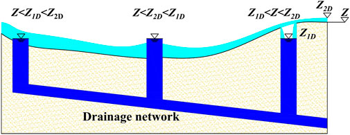
FIGURE 1. Exchange conditions of vertical flow in the 1D–2D coupled model.

The orifice equation (Eq. 7) is used to calculate the overflow from the sewer pipe to the surface when the water depth in inlets exceeds the surface water elevation.

$Q_{over}=c_{o}A{}_i\sqrt{2g\left(Z_{1D}-Z_{2D}\right).}(7)$

Here, $Q_{over}$ represents the overflow from the sewer system to the surface.

In this work, the source term method was used to couple the 1D model and the 2D model. $R$ is the source or sink of mass caused by rainfall, infiltration, and water exchange with the sewer system. Hence, the rainfall source term can be expressed using the following equation (Li et al., 2020):

$R=i-f_c-c\left(Q_{in}-Q_{over}\right),(8)$

where $i$ is the rainfall, $f_c$ represents the infiltration, $c\left(Q_{in}-Q_{over}\right)$ denotes the water exchange with the sewer system, and c is a correction factor to account for the difference in unit and grid size.

2.2 Existing method for computing the drainage effect

In the existing method, in addition to considering the basic soil infiltration (Figure 2), extra mass is subtracted from the entire area to represent the drainage system capacity. Eq. 9 is applied in the existing method (Li et al., 2020).

$R_E=i-f_c-E.(9)$

Here, $R_E$ represents the rainfall source term in the existing method; $E$ represents the subtracted mass rate (mm/h).

FIGURE 2

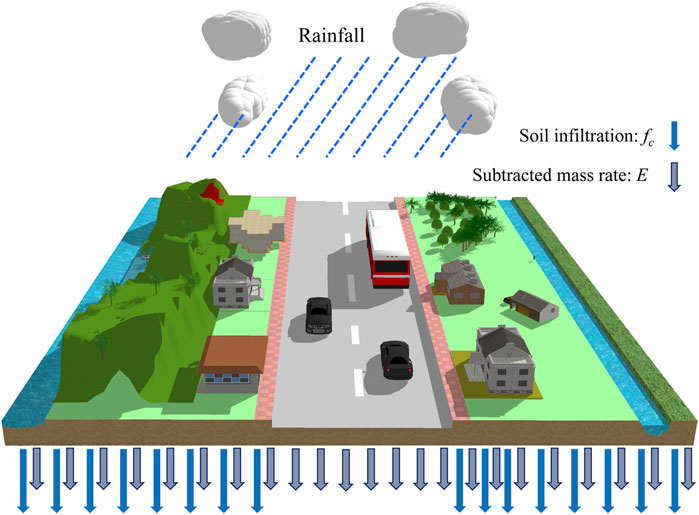
FIGURE 2. Schematic diagram of the existing method.

2.3 New method for computing the drainage effect

To be more specific, the actual rainfall–runoff process consists of generation and confluence. In addition, surface water usually travels a long distance, such as over roofs and through gardens, before it can flow into the drainage system (Li et al., 2020). The drainage system, consisting of pipes and gutters, is mainly built under the road line. Thus, extra subtraction is applied to the mass flow into the road area to represent the capacity of the drainage pipes (Figure 3). This new method is described by Eq. 10.

$R_N=\left\{\begin{array}{l}i-N\mathrm{i}\mathrm{f}\mathrm{f}\mathrm{l}\mathrm{a}\mathrm{g}=\mathrm{R}\mathrm{o}\mathrm{a}\mathrm{d}\\ i-f_c\mathrm{i}\mathrm{f}\mathrm{f}\mathrm{l}\mathrm{a}\mathrm{g}\ne \mathrm{R}\mathrm{o}\mathrm{a}\mathrm{d}\end{array}\right..(10)$

Here, $R_N$ denotes the rainfall source term in the new method; the flag represents the type of land use. In the new method, the mass is subtracted only in land of the road type, and $N$ represents the mass subtraction rate for roads that is applied in the new method (mm/h).

$N=c_N\frac{N_i}{N_r}{c}_w{C}_i{h}_{2D}\sqrt{2g{h}_{2D}}/A_{cell.}(11)$

FIGURE 3

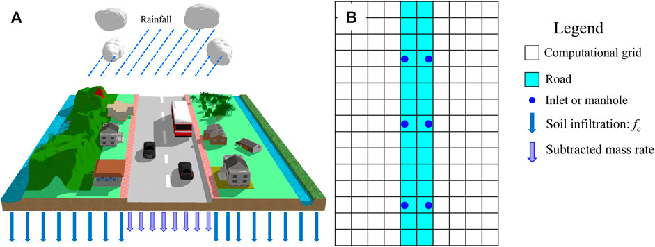
FIGURE 3. Schematic diagram of the new method. (A) Schematic diagram of road drainage. (B) Calculation method for the subtracted mass rate N.

Here, $c_N$ represents the correction factor of the new method; $N_i$ is the inlet number, which can be estimated by the length of the road; $N_r$ is the grid number of the road land use; $c_w$ represents the weir coefficient; $C_i$ denotes the perimeter of the inlet; $g$ is the acceleration of gravity; $h_{2D}$ represents the water level at the surface; and $A_{cell}$ is the area of a 2D cell.

Figure 4 shows a flow chart for the existing and new methods. First, fundamental data are provided as inputs to the different methods, together with the digital elevation model (DEM), the initial conditions, and the land use type. Subsequently, rainfall and infiltration are calculated. Next, the rainfall term is modified to reflect the capacity of the drainage pipes. Both of the two methods of approximation correct the rainfall term in the model to reflect the drainage capacity. The rainfall term for the entire area is reduced under the existing method, while the mass is reduced only in road areas in the new method. Finally, the fluxes, slope, and friction terms are calculated in the same way in both methods.

FIGURE 4

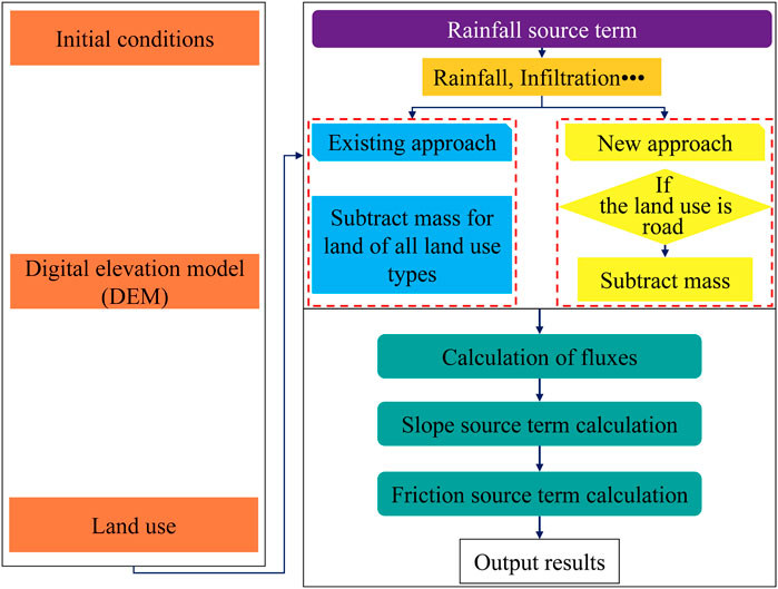
FIGURE 4. Methodology diagram for the two approximation methods.

3 Case study

In order to examine the representations of drainage capacity computed by each of the two approximation methods in the simulation of rainfall–runoff–drainage processes, the idealized urban catchment case (Li et al., 2020) and the case of the Fengxi urban area were used as case studies for analysis. Their results were compared with those of the 1D–2D coupled model.

3.1 Basic data

Both cases were taken from Li et al. (2020). The size of the ideal urban catchment is 284 m and 240 m (Figure 5), which is based on the size of an actual urban catchment. The longitudinal slope i₁ is 0.003, and the transverse slope i₂ is 0.005. The cross-section is shown in Figure 5B. The width is composed of a 130-m-wide confluence area on both sides and a 24-m-wide road, and there is a slope of i₃ = 0.02 from the middle to the side of the road. There are 20 inlets, one outlet, and 20 pipelines in the idealized catchment. The inlet size is 0.4 × 0.7 m, and the pipe diameter is 0.8 m. The drainage pipe layout is shown in Figure 5A. The infiltration of the entire catchment is 0 mm/h. All boundaries except exits are closed boundaries. The Manning value of the road is 0.014, and the value on both sides is 0.03. The computational domain is discretized to a resolution of 1 m (Li et al., 2020).

FIGURE 5

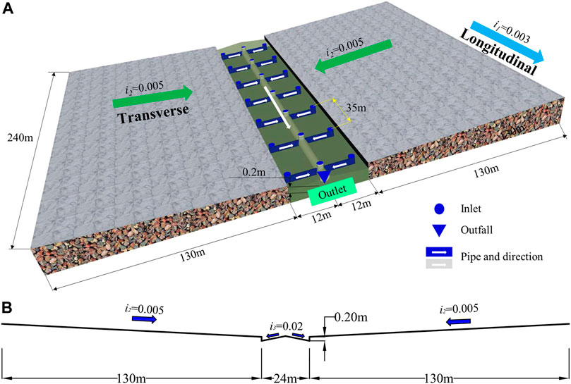
FIGURE 5. Sketch map of the ideal test case. (A) Drainage system layout and stereogram. (B) Cross-section.

The second test case is part of Fengxi New City, located in Xixian New Area, Shaanxi Province, China (Figure 6A). It is a typical urban region with an area of 47.35 hm². The input data of the model included the DEM with 2 m resolution (Figure 6B), infiltration rates, and Manning coefficients (Table 1). The Manning coefficients and soil infiltration rates of different underlying surfaces were based on Li et al. (2020). Figure 6C shows the five basic land use types of the catchment: grassland, roads, bare land, buildings, and forests. The layout of drainage pipes in the catchment was based on the actual layout, as shown in Figure 6D. This layout included 81 inlets, 81 pipes, and four outfalls. The diameter of the pipes was 0.8 m. This information was provided by the Technology Research Center for Sponge City of Fengxi New City.

FIGURE 6

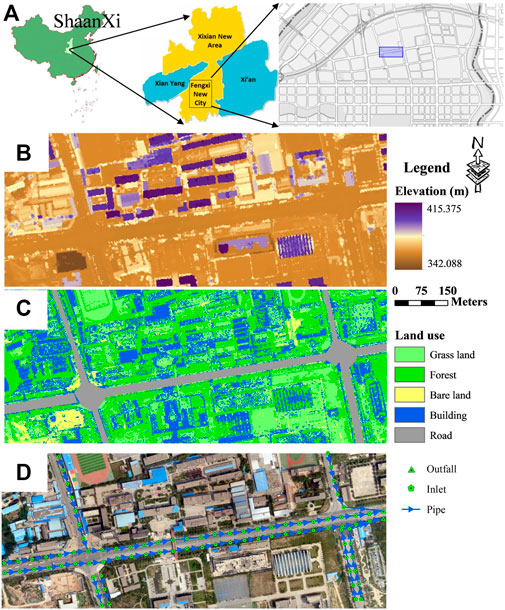
FIGURE 6. Actual test case. (A) Location map. (B) DEM map. (C) Land use map. (D) Layout of the drainage system and digital orthophoto map.

TABLE 1

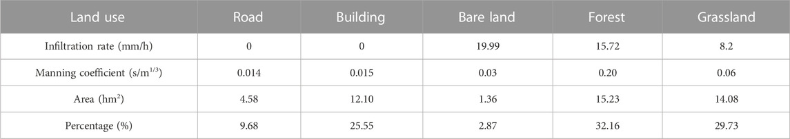
TABLE 1. Infiltration rates, Manning coefficients, and percentage of land under different types of use in the coupled model.

3.2 Parameter calibration

For calibration of the subtracted values used by each of the two approximation approaches, a rainfall event with an intensity of 60 mm/h and a duration of 1 h was used; the simulation period was 2 h. Under the aforementioned rainfall event, the following three steps were followed to calibrate the parameters:

Step 1. the coupled model method to obtain the discharge amount at the outlet, and these results were taken as the standard for calibration.

Step 2. The subtracted values under each of the two approximation methods were adjusted until the difference in discharge volumes between each of the two approaches and the coupled model at the second hour was less than 1%.

Step 3. subtracted values of E = 26.0 mm/h under the existing method and c_N = 1.15, N_i = 21, N_r = 5,760 under the new method were obtained.

Furthermore, the error in discharge volume was −1% between the existing method and the coupled model, and 1% between the new method and the coupled model. To reflect the drainage effect, a simulation with no drainage pipes and no infiltration in the urban area was run. Figure 7 depicts the progress of a rainstorm event and the discharge volume at the road’s outlet under various scenarios.

In regard to the real case examined, a measured rainfall hyetograph (Figure 8) represents a particular rainfall event that occurred in the actual urban catchment. This event lasted 7.5 h, starting at 00:30 AM and continuing until 08:00 AM on 25 August 2016. The total rainfall was 66 mm, the maximum hourly rainfall for 3.1 h was 65.4 mm/h, and the return period of this storm event is about 50 years (Li et al., 2020). According to inundation data observed at the site, the inundation area measured in the 5th hour was approximately 1,600 m². The calibration process used in the ideal test case was also carried out for this scenario.

The result of the coupled model for inundation area at the 5th hour was 1,656 m². This value was in good agreement with the measured data, thus validating the coupled model. Finally, after many trial calculations, when the reduction rate for the entire area in the existing method was calibrated to 9.0 mm/h and the parameters of the new method were calibrated to c_N = 0.26, N_i = 82, N_r = 11,461, the inundation extents computed under each approach at the 5th hour were 1,652 m² and 1,616 m², respectively. Compared with the measured data, the error in both results was less than 5%, which represents good agreement with the measured data. The time course of the inundation area under each of the different methods is shown in Figure 8. This indicates that the new method is superior, because its representation of the later flooding process is closer to that of the coupled model.

FIGURE 7

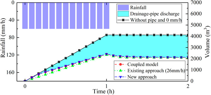
FIGURE 7. Volume time course and rainfall process under various scenarios.

FIGURE 8

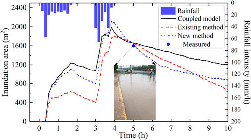
FIGURE 8. Measured hyetography for calibration and simulation results of the time course of inundation area for various methods under the actual catchment scenario.

3.3 Storm

Design storms (Eq. 12) defined for Xi’an County, Shaanxi Province (Bi et al., 2015), with return periods of 2, 5, 10, 30, 50, and 100 years and a duration time of 2 h (Figure 9) were employed as rainfall input data.

$q_r=\frac{2210.87\times \left(1+2.915\times \lg p\right)}{{\left(t+21.933\right)}^{0.974}},(12)$

where q_r denotes the rainfall intensity (L/(s·hm²)); p is the return period in years; and t denotes rainfall duration in min.

FIGURE 9

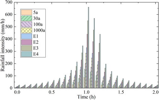
FIGURE 9. Design storm hyetography for various return periods.

3.4 Modeling accuracy evaluation index

The relative error (RE) of the inundation volume was used to measure the difference between volume values under the coupled model and under each of the approximation approaches in order to describe the effects of the two methods statistically and quantitatively. The equation for RE is as follows:

$RE=\left(V_c-V_a\right)/V_c*100\%,(13)$

where $V_c$ represents the inundation volumes (m³) simulated by the coupled model and $V_a$ represents the value in the approximation method. $RE$ < 0 indicates that the approximation method overestimated the capacity of the drainage pipes, and $RE$ > 0 indicates that it underestimated their capacity.

To statistically and quantitatively describe the effects of the approximation methods on the time shift (TS) of the inundation rise and peak, the TS is assigned to quantify the difference of the inundation rising and peak between the coupled model and the two methods. The formulation of TS is as follows:

$TS=T_c-T_a,(14)$

where $TS$ represents the time shift; $T_c$ represents the occurrence time (minutes) of the inundation rise or peak in the coupled model; and $T_a$ represents the occurrence time under the approximation method.

4 Results

4.1 Idealized urban catchment

The time course of the inundation volume over the entire idealized urban catchment area and the peak volume, as calculated via different methods (coupled model, existing method, and new method), are presented in Figure 10 and Table 2. RE between the coupled model and the existing method ranged between −9.74% and 60.36%, decreasing with the increase in rainfall return period. The existing method overestimated the capacity of the drainage pipes under rainfall with a return period of less than 30 years and underestimated drainage capacity with a return period of more than 50 years.

FIGURE 10

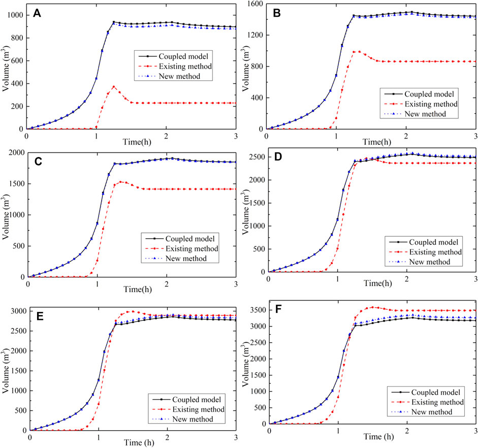
FIGURE 10. Simulated volume time course for the entire area under three different methods for the idealized urban catchment in the case of rainfall events with return periods of (A) 2 years, (B) 5 years, (C) 10 years, (D) 30 years, (E) 50 years, and (F) 100 years.

TABLE 2

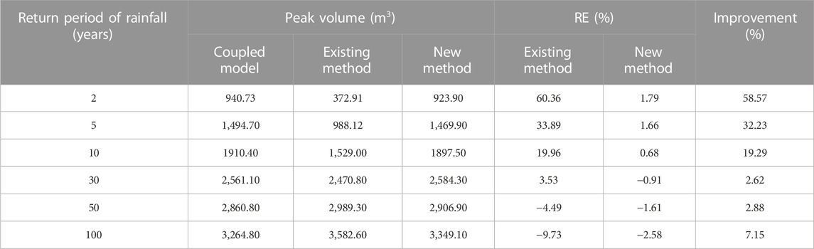
TABLE 2. Comparison of peak volume estimates under different methods for the idealized urban catchment case study.

RE values between the coupled model and the new method were 1.79%, 1.66%, 0.68%, −0.91%, −1.61%, and −2.58% for rainfall events with return periods of 2, 5, 10, 30, 50, and 100 years, respectively. Similar to the results for the existing method, RE for the new method decreased with the increase in rainfall return period. The new method overestimated the capacity of the drainage pipes under rainfall with a return period of less than 10 years and underestimated drainage capacity with a return period of more than 30 years. Overall, RE for the new method was no more than 3%, which is very small. Compared with the existing method, the new method improves the estimate of peak volume by 2.62%–58.57% for rainfall events with different return periods. The results clearly show that the new method is more effective than the existing one (Li et al., 2020; Hou et al., 2021).

Moreover, the runoff delay under the different methods can be clearly observed in Figure 10. Compared with the coupled model, the TS of the inundation rise under the existing method was approximately 35–40 min for different return periods. The TS of the inundation peak was approximately 35–45 min for different return periods (Figure 11A). There was no runoff delay for the inundation rise and peak under the new method; that is, TS was 0. The phenomenon of runoff delay would directly reduce the formation of inundations and occurrence of flood peaks in urban catchments (Wang et al., 2018). The reason for this is that the runoff would not occur until half an hour after the rainfall under non-constant rainfall with different return periods under the existing method, because the volume of rainfall up to that point would be less than the subtracted value of 26.0 mm/h over the entire area. However, under the new method, runoff could be generated on both sides of the road, so such a delay is not inevitable (Li et al., 2020). There are also runoff delays under the existing method in the process of calibrating parameters under constant rainfall; these delays are of approximately 5 min. Hence, the simulation results are consistent with those of the calibration process.

FIGURE 11

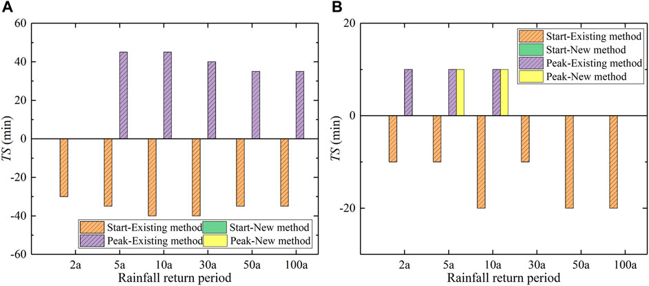
FIGURE 11. TS of the inundation start and peak under two approximation methods (A) in the idealized urban catchment and (B) in the Fengxi urban catchment.

4.2 Fengxi urban catchment

Design storms and the three methods were also imported into the model in order to simulate the runoff process in the actual urban catchment with a simulation duration of 10 h. Figure 12 shows the time course of water volume over the entire urban catchment area under rainfall with different return periods. The peak volume calculated by each of the different methods for the actual urban catchment area is presented in Table 3. The results clearly demonstrate that there are differences between the existing method and the new method. RE for both methods decreased with increase in the rainfall return period. In addition, the peak volume values under both the existing method and the new method were less than that of the coupled model for rainfall events with various return periods, which means that the two methods overestimated the drainage capacity of the sewer pipes. Compared to the peak volume of the coupled model, the range of RE for the existing and new methods was 5.57%–39.79% and 2.00%–6.93%, respectively. The improvement provided by the new method compared to the existing method ranged from 3.57%–32.87% for rainfall events with different return periods. Furthermore, RE for the new method was less than 7% in the actual urban catchment under various scenarios. Moreover, compared with the coupled model, the TS of the inundation rise under the existing method was approximately 10–20 min for different return periods. The TS of the inundation peak was approximately 0–10 min for different return periods (Figure 11B). The TS of inundation peak is 10 min under the rainfall with 5 and 10 years return period in the actual urban catchment. The trend of the result was consistent with the findings for the idealized urban catchment.

FIGURE 12

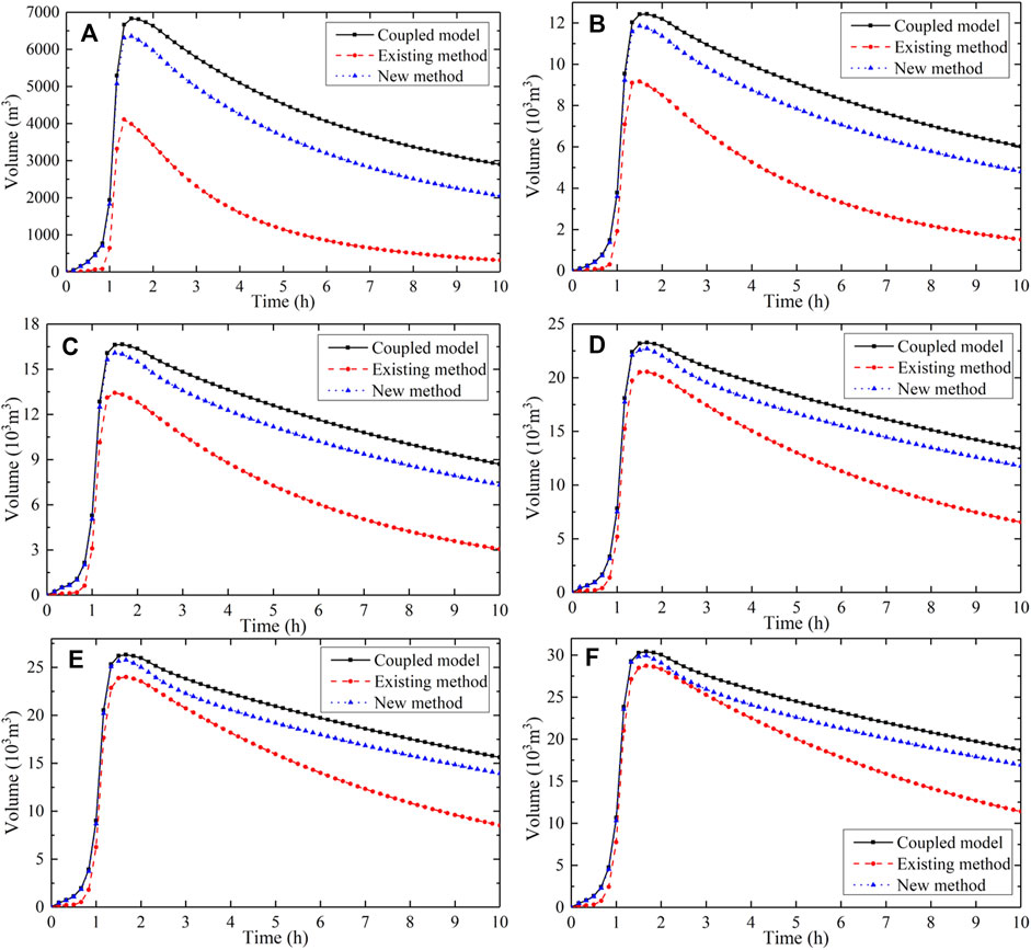
FIGURE 12. Comparison of the water volume time course in the actual urban catchment scenario under different methods in the case of rainfall events with return periods of (A) 2 years, (B) 5 years, (C) 10 years, (D) 30 years, (E) 50 years, and (F) 100 years.

TABLE 3

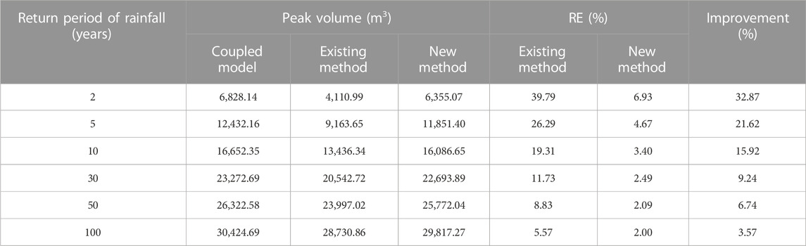
TABLE 3. Inundation peak volume under different methods for the actual urban catchment case study.

5 Discussion and conclusion

The use of 1D–2D coupled models represents a critical approach for evaluating urban flooding. Nonetheless, a significant deficiency in data pertaining to municipal sewer systems impedes the full utilization of flood modeling (Hou et al., 2021; Li et al., 2022). The utilization of approximation methods to reflect the effects of discharge pipes can provide a more accurate representation of surface rainfall flooding events in circumstances where the underlying mechanisms of subterranean sewer network water flow are disregarded (Li et al., 2020). However, the existing approximation methods for this drainage effect are inconsistent with the actual rainfall–runoff process, and the simulation error is relatively large. As a result, improving the accuracy of the values calculated via such an approximation method is crucial to accurately simulate the urban flood process. In this study, a novel road-drainage method is presented, which is more consistent with the physics of the rainfall–runoff process. This method does not require the construction of underground pipe network data, and the corresponding reduction in the rainfall source term for areas of road in the 2D model can reflect the drainage effect.

The proposed method was evaluated via simulation of an ideal and an actual urban catchment. Due to a lack of monitoring data, the calculation results of the coupled model were used as the benchmark in this paper. First, a single rainfall event was used to calibrate the relevant parameters; subsequently, the effects of the new method on the results of simulations of storm-related flooding were evaluated for rainfall events with return periods of 2, 5, 10, 30, 50, and 100 years. In the ideal case study, a scenario with constant rainfall of 60 mm/h was used to calibrate the correction parameters of the new method and the existing method. To increase reliability, the subtracted values of the two methods were also calibrated under rainfall events with an intensity of 30 mm/h and 90 mm/h for the idealized urban catchment. Moreover, the same scenario was simulated under rainfall events with return periods of 2, 5, 10, 30, 50, and 100 years. All the results showed that the new method produces smaller RE values than the existing method for various rainfall events.

However, the new method is not able to reflect the backflow and overflow processes of the drainage piping. Overflow usually occurs when the drainage capacity of the pipe network is insufficient, and rainwater flows back from the underground pipe network to the surface under water pressure. Hou et al. (2021) proposed an approximate simulation method based on non-linear reservoirs to simulate the overflow process, but this method also needs the support of pipe network data. Constructing underground pipe network data according to urban characteristics is also an effective way to solve this problem, but these methods are relatively complicated, and the vast amount of pipe network data required also brings new challenges to flood simulation for large-scale urban areas (Chegini and Li, 2022). Further research is needed for more advanced methods to reflect the drainage system of areas where the data are unavailable.

The results showed that RE between the new method and the coupled model decreased with increase in the return period for both urban catchment case studies. RE for the inundation peak ranged from 1.72% to 2.58% for rainfall return periods ranging from 2 years to 100 years in the idealized urban catchment scenario, and from 6.93% to 2.00% in the actual urban catchment scenario. This means that the approximation method with a fixed parameter exhibited the best adaptability for modeling of rainfall events with a certain return periods. For example, RE was smallest when c = 1.15 in the new method for a rainfall event with a 10-year return period in the idealized urban catchment. Additionally, under this method, drainage system capacity was overestimated when the return period of the rainfall was less than 10 years and underestimated when the return period was greater than 10 years. Similar patterns were also found for the existing method. One reason for this could be that the surface water depth is variable under rainfall with different return periods. The water depth at the inlet node is considered in the coupled model, while the water depth over the entire road is considered in the new method (Li et al., 2020; Hou et al., 2021). Generally, the subtracted values, which may be related to both the calibrated rainfall and the pipe diameter of different methods, need to be studied further. The actual situation may be more complicated, and in-depth research will continue in the future. An important direction for further work might be to investigate the possibility of adopting variable parameters for approximation methods in scenarios representing rainfall events with different return periods.

To summarize, the main findings and implications of this study are as follows. 1) A method for approximate computation of drainage capacity for urban flood modeling is proposed; this is named the road-drainage method. 2) Relative error in inundation peak volume between the proposed method and the coupled model is less than 3% in an idealized urban catchment and 7% in an actual urban catchment. 3) The TS of the inundation rise and peak is 0 in an idealized urban catchment, and the TS of the inundation peak is only 10 min under rainfall events with 5- and 10-year return periods in an actual urban catchment. 4) The simulation accuracy of peak volume is improved by 2.62%–58.75% and 3.57%–32.87% compared with the existing method for the idealized urban catchment scenario and the actual urban catchment scenario, respectively. In addition, TS is reduced by 10–45 min over various scenarios. The results of the new method indicate that it could reflect the influence of the drainage system more accurately than the existing method in the ideal urban catchment and an actual urban catchment.

Overall, the simulation results show that the road-drainage method is a more reliable and efficient approach to modeling of drainage capacity than the existing method. This finding is useful for the modeling of urban areas with inaccessible drainage system data. In particular, the road-drainage method holds great promise as a solution for simulating urban flooding in areas where drainage system data are not available. It has the potential to support large-scale urban hydrological modeling, making it an invaluable tool for predicting and preventing the impacts of flood events. Furthermore, the application of this method to large-scale regions will be investigated. More advanced approximation methods that can incorporate backflow and overflow processes are also a research direction for the future.

Data availability statement

The original contributions presented in the study are included in the article/supplementary material; further inquiries can be directed to the corresponding authors.

Author contributions

DL carried out the numerical simulation and drafted the original manuscript. JH and RS conducted the analyses and conceived the manuscript. YT reviewed and polished the manuscript. BL and TW performed the data analyses and edited the manuscript. All authors have read and agreed to the published version of the manuscript.

Funding

This work is partly supported by the National Natural Science Foundation of China (Grant Nos. 52079106 and 52009104), the Key R&D Program of Ningxia of China (Grant No. 2022BEG02020), Key Science and Technology Projects of PowerChina (DJ-ZDXM-2022-41), and major company-level Science and Technology Projects of Northwest Engineering Corporation Limited, PowerChina (XBY-ZDKJ-2022-9).

Conflict of interest

Author RS was employed by Ningxia Capital Sponge City Construction & Development Co., Ltd.

The authors declare that this study received funding from Northwest Engineering Corporation Limited, Power China. The funder had the following involvement in the study: basic data collection.

The remaining authors declare that the research was conducted in the absence of any commercial or financial relationships that could be construed as a potential conflict of interest.

Publisher’s note

All claims expressed in this article are solely those of the authors and do not necessarily represent those of their affiliated organizations, or those of the publisher, the editors, and the reviewers. Any product that may be evaluated in this article, or claim that may be made by its manufacturer, is not guaranteed or endorsed by the publisher.

References

Adeogun, A. G., Daramola, M. O., and Pathirana, A. (2015). Coupled 1D-2D hydrodynamic inundation model for sewer overflow: Influence of modeling parameters. Water Sci. 29 (2), 146–155. doi:10.1016/j.wsj.2015.12.001

CrossRef Full Text | Google Scholar

Agency, E. (2013). Updated flood map for surface water-national scale surface water flood mapping methodology. Bristol, UK: Environment Agency.

Google Scholar

Ali, M., Khan, S. J., Aslam, I., and Khan, Z. (2011). Simulation of the impacts of land-use change on surface runoff of Lai Nullah Basin in Islamabad, Pakistan. Landsc. Urban Plan. 102 (4), 271–279. doi:10.1016/j.landurbplan.2011.05.006

CrossRef Full Text | Google Scholar

Avand, M., Kuriqi, A., Khazaei, M., and Ghorbanzadeh, O. (2022). DEM resolution effects on machine learning performance for flood probability mapping. J. Hydro-environment Res. 40, 1–16. doi:10.1016/j.jher.2021.10.002

CrossRef Full Text | Google Scholar

Bi, X., Dang, C.-q., and Cheng, L. (2015). Study on compiling rainstorm intensity formula in xi'an urban. J. Anhui Agri 43 (26), 223–225+228. doi:10.13989/j.cnki.0517-6611.2015.26.212

CrossRef Full Text | Google Scholar

Bladé, E., Gómez-Valentín, M., Dolz, J., Aragón-Hernández, J. L., Corestein, G., and Sánchez-Juny, M. (2012). Integration of 1D and 2D finite volume schemes for computations of water flow in natural channels. Adv. Water Resour. 42, 17–29. doi:10.1016/j.advwatres.2012.03.021

CrossRef Full Text | Google Scholar

Chang, T.-J., Wang, C.-H., and Chen, A. S. (2015). A novel approach to model dynamic flow interactions between storm sewer system and overland surface for different land covers in urban areas. J. Hydrology 524, 662–679. doi:10.1016/j.jhydrol.2015.03.014

CrossRef Full Text | Google Scholar

Chegini, T., and Li, H. Y. (2022). An algorithm for deriving the topology of below-ground urban stormwater networks. EGUsphere 2022, 1–30. doi:10.5194/egusphere-2022-90

CrossRef Full Text | Google Scholar

Chen, A., Djordjević, S., Leandro, J., and Savic, D. (2007). The urban inundation model with bidirectional flow interaction between 2D overland surface and 1D sewer networks.

Google Scholar

Chen, W., Huang, G., Zhang, H., and Wang, W. (2018). Urban inundation response to rainstorm patterns with a coupled hydrodynamic model: A case study in haidian island, China. J. Hydrology 564, 1022–1035. doi:10.1016/j.jhydrol.2018.07.069

CrossRef Full Text | Google Scholar

Debarati, G.-S., Philippe, H., Pascaline, W., and Regina, B. (2016). Annual disaster statistical review 2016: The numbers and trends. Brussels: Université Catholique de Louvain.

Google Scholar

Fan, Y., Ao, T., Yu, H., Huang, G., and Li, X. (2017). A coupled 1D-2D hydrodynamic model for urban flood inundation. Adv. Meteorology 2017, 1–12. doi:10.1155/2017/2819308

CrossRef Full Text | Google Scholar

Hou, J., Wang, R., Li, G., and Li, G. (2018). High-performance numerical model for high-resolution urban rainfall-runoff process based on dynamic wave method. J. Hydroelectr. Eng. 37 (3), 40–49.

Google Scholar

Hou, J., Yang, D., Li, B., Bai, G., Xia, J., Wang, Z., et al. (2021). Approximate method for evaluating the drainage process of an urban pipe Netw. Unavailable Data. 147(10), 04021043. doi:10.1061/(ASCE)IR.1943-4774.0001607

CrossRef Full Text | Google Scholar

I., D. H. S. (2014). MIKE 21 FLOW MODEL hydrodynamic module scientific documentation. Denmark: Danish Hydraulic Institute.

Google Scholar

Ilderomi, A. R., Vojtek, M., Vojteková, J., Pham, Q. B., Kuriqi, A., and Sepehri, M. J. A. J. o. G. (2022). Flood prioritization integrating picture fuzzy-analytic hierarchy and fuzzy-linear assignment model. Arab. J. Geosci. 15 (13), 1185. doi:10.1007/s12517-022-10404-y

CrossRef Full Text | Google Scholar

Jang, J.-H., Chang, T.-H., and Chen, W.-B. (2018). Effect of inlet modelling on surface drainage in coupled urban flood simulation. J. Hydrology 562, 168–180. doi:10.1016/j.jhydrol.2018.05.010

CrossRef Full Text | Google Scholar

Jia, L., Yu, K.-x., Li, Z.-b., Li, P., Zhang, J.-z., Wang, A.-n., et al. (2022). Temporal and spatial variation of rainfall erosivity in the Loess Plateau of China and its impact on sediment load. CATENA 210, 105931. doi:10.1016/j.catena.2021.105931

CrossRef Full Text | Google Scholar

Klipalo, E., Besharat, M., and Kuriqi, A. (2022). Full-scale interface friction testing of geotextile-based flood defence structures. Def. Struct. 12 (7), 990. doi:10.3390/buildings12070990

CrossRef Full Text | Google Scholar

Kratt, C. B., Woo, D. K., Johnson, K. N., Haagsma, M., Kumar, P., Selker, J., et al. (2020). Field trials to detect drainage pipe networks using thermal and RGB data from unmanned aircraft. Agric. Water Manag. 229, 105895. doi:10.1016/j.agwat.2019.105895

CrossRef Full Text | Google Scholar

Kuriqi, A., and Hysa, A. (2022). “Multidimensional aspects of floods: Nature-based mitigation measures from basin to river reach scale,” in Nature-based solutions for flood mitigation: Environmental and socio-economic aspects. Editors C. S. S. Ferreira, Z. Kalantari, T. Hartmann, and P. Pereira (Cham: Springer International Publishing), 11–33.

Google Scholar

Lashford, C., Rubinato, M., Cai, Y., Hou, J., Abolfathi, S., Coupe, S., et al. (2019). SuDS & Sponge cities: A comparative analysis of the implementation of pluvial flood management in the UK and China. Sustainability 11 (1), 213. doi:10.3390/su11010213

CrossRef Full Text | Google Scholar

Li, D., Hou, J., Xia, J., Tong, Y., Yang, D., Zhang, D., et al. (2020). An efficient method for approximately simulating drainage capability for urban flood. Front. Earth Sci. 8. doi:10.3389/feart.2020.00159

CrossRef Full Text | Google Scholar

Li, D., Hou, J., Zhang, Y., Guo, M., and Zhang, D. (2022). Influence of time step synchronization on urban rainfall-runoff simulation in a hybrid CPU/GPU 1D-2D coupled model. Water Resour. Manag. 36, 3417–3433. doi:10.1007/s11269-022-03158-5

CrossRef Full Text | Google Scholar

Liang, Q., and Marche, F. (2009). Numerical resolution of well-balanced shallow water equations with complex source terms. Adv. Water Resour. 32 (6), 873–884. doi:10.1016/j.advwatres.2009.02.010

CrossRef Full Text | Google Scholar

Martinez, C., Sanchez, A., Toloh, B., and Vojinovic, Z. J. W. R. M. A. I. J. (2018). Published for the European water resources AssociationMulti-objective evaluation of urban drainage networks using a 1D/2D flood inundation model. Water Resour. manage. 32 (13), 4329–4343. doi:10.1007/s11269-018-2054-x

CrossRef Full Text | Google Scholar

Rossman, L. A. (2009). Storm Water Management Model: User's Manual Version 5.0. Washington, DC: Environmental Protection Agency.

Google Scholar

SOLUTIONS.X.P (2013). XP-SWMM stormwater and wastewater management model. Newbury, UK: Getting Started ManualXP SOLUTIONS.

Google Scholar

Tariq, A., Shu, H., Kuriqi, A., Siddiqui, S., Gagnon, A. S., Lu, L., et al. (2021). Characterization of the 2014 indus river flood using hydraulic simulations and satellite images. Remote Sens. (Basel). 13 (11), 2053. doi:10.3390/rs13112053

CrossRef Full Text | Google Scholar

Tscheikner-Gratl, F., Caradot, N., Cherqui, F., Leitão, J. P., Ahmadi, M., Langeveld, J. G., et al. (2019). Sewer asset management – state of the art and research needs. Urban Water J. 16 (9), 662–675. doi:10.1080/1573062X.2020.1713382

CrossRef Full Text | Google Scholar

Wang, Y., Chen, A. S., Fu, G., Djordjević, S., Zhang, C., and Savić, D. A. (2018). An integrated framework for high-resolution urban flood modelling considering multiple information sources and urban features. Environ. Model. Softw. 107, 85–95. doi:10.1016/j.envsoft.2018.06.010

CrossRef Full Text | Google Scholar

Wu, X., Wang, Z., Guo, S., Liao, W., Zeng, Z., and Chen, X. (2017). Scenario-based projections of future urban inundation within a coupled hydrodynamic model framework: A case study in dongguan city, China. J. Hydrology 547, 428–442. doi:10.1016/j.jhydrol.2017.02.020

CrossRef Full Text | Google Scholar

Xia, X., Liang, Q., Ming, X., and Hou, J. (2017). An efficient and stable hydrodynamic model with novel source term discretization schemes for overland flow and flood simulations. Water Resour. Res., 53, 3730–3759. doi:10.1002/2016WR020055

CrossRef Full Text | Google Scholar

Zhang, S., and Pan, B. (2014). An urban storm-inundation simulation method based on GIS. J. Hydrology 517, 260–268. doi:10.1016/j.jhydrol.2014.05.044

CrossRef Full Text | Google Scholar

Glossary

1D One-dimensional

2D Two-dimensional

SWMM Storm Water Management Model

SWEs Shallow water equations

USEPA United States Environmental Protection Agency

DEM Digital elevation model

RE Relative error of the inundation volume

TS Time shift of the inundation rise and peak

t Time

subscript x x-axis of the Cartesian plane

subscript y y-axis of the Cartesian plane

q Variable vector

f Flux vector of the x direction

g Flux vector of the y direction

h Depth of water

q_x Single-width discharge in the x-axis direction

q_y Single-width discharge in the y-axis direction

S Source vector

S_b Slope source terms

S_f Friction source terms

u Current velocity in the x direction

v Current velocity in the y direction

C_f Chezy’s coefficient

n Manning coefficient

R Rainfall term

$\mathit{i}$ Rainfall

${\mathit{f}}_{\mathit{c}}$ Infiltration

$\mathit{A}$ Flow cross-sectional area

$\mathit{Q}$ Flow rate

$\mathit{g}$ Acceleration of gravity

$\mathit{H}$ Hydraulic head of water in the conduit (Z + Y)

Z Conduit invert elevation

Y Conduit water depth

${\mathit{S}}_{\mathit{f}\mathbf{1}\mathit{D}}$ Friction slope (head loss per unit length) in the pipe

${\mathit{Q}}_{\mathit{i}\mathit{n}}$ Flow from the 2D surface to the sewer

${\mathit{c}}_{\mathit{w}}$ Weir coefficient

${\mathit{c}}_{\mathit{o}}$ Orifice coefficient

${\mathit{C}}_{\mathit{i}}$ Perimeter of the inlet

${\mathit{h}}_{\mathbf{2}\mathit{D}}$ Water level at the surface

${{\mathit{Z}}_{\mathit{b}}}_{\mathbf{2}\mathit{D}}$ Bed elevation of the surface

${\mathit{Z}}_{\mathbf{2}\mathit{D}}$ Surface water elevation

${\mathit{Z}}_{\mathbf{1}\mathit{D}}$ Inlet water elevation

${\mathit{A}}_{\mathit{i}}$ Inlet area

${\mathit{Q}}_{\mathit{o}\mathit{v}\mathit{e}\mathit{r}}$ Overflow from the sewer system to the surface

c Correction factor for the difference in unit and grid size

${\mathit{R}}_{\mathit{E}}$ Rainfall source term in the existing method

E Subtracted mass rate in the existing method

${\mathit{R}}_{\mathit{N}}$ Rainfall source term in the new method

N Subtracted mass rate for road areas in the new method

${\mathit{c}}_{\mathit{N}}$ Correction factor in the new method

${\mathit{N}}_{\mathit{i}}$ Inlet number

${\mathit{N}}_{\mathit{r}}$ Grid number of the road land use

${\mathit{A}}_{\mathit{c}\mathit{e}\mathit{l}\mathit{l}}$ Area of a 2D cell

q_r Rainfall intensity

p Return period