Estimation of hazardous and noxious substance (toluene) thickness using hyperspectral remote sensing

A hazardous noxious substance (HNS) spill accident is one of the most devastating maritime disasters as it is accompanied by toxicity, fire, and explosions in the ocean. To monitor an HNS spill, it is necessary to develop a remote sensing–based HNS monitoring technique that can observe a wide area with high resolution. We designed and performed a ground HNS spill experiment using a hyperspectral sensor to detect HNS spill areas and estimate the spill volume. HNS images were obtained by pouring 1 L of toluene into an outdoor marine pool and observing it with a hyperspectral sensor capable of measuring the shortwave infrared channel installed at a height of approximately 12 m. The pure endmember spectra of toluene and seawater were extracted using principal component analysis and N-FINDR, and a Gaussian mixture model was applied to the toluene abundance fraction. Consequently, a toluene spill area of approximately 2.4317 m² was detected according to the 36% criteria suitable for HNS detection. The HNS thickness estimation was based on a three-layer two-beam interference theory model. Because toluene has a maximum extinction coefficient of 1.3055 mm at a wavelength of 1,678 nm, the closest 1,676.5 nm toluene reflectance image was used for thickness estimation. Considering the detection area and ground resolution, the amount of leaked toluene was estimated to be 0.9336 L. As the amount of toluene used in the actual ground experiment was 1 L, the accuracy of our estimation is approximately 93.36%. Previous studies on HNS monitoring based on remote sensing are lacking in comparison to those on oil spills. This study is expected to contribute to the establishment of maritime HNS spill response strategies in the near future based on the novel hyperspectral HNS experiment.

1 Introduction

According to the Protocol on Preparedness, Response and Co-operation to Pollution Incidents by Hazardous and Noxious Substances, a hazardous and noxious substance (HNS) is any chemical substance, except oils, that pollutes the ocean by destroying the environment or is harmful to humans and marine life (Neuparth et al., 2011). Owing to the development of the petrochemical industry, there are approximately 6,000 types of HNSs, which are classified into bulk liquids, gases, solids in bulk, and packaged goods. HNSs are transported worldwide via vessels such as oil tankers, chemical tankers, container ships, liquefied petroleum gas, liquefied natural gas tankers, and bulk tankers (Cho et al., 2013). Oil spill accidents have occurred continuously with a wide distribution over the global ocean, especially in coastal waters (Chen et al., 2019). The spatial distribution of accident sites in the western North Pacific region where more than 10 tons of oil and HNSs were spilled from 1990 to 2019 is shown in Figure 1. During this period, 372 oil spills and 49 HNS spills occurred, primarily near the coast. Although the number of HNS accidents is smaller than that of oil spills, the various physicochemical properties of HNSs, such as flammability, explosiveness, toxicity, and persistence, can cause severe human, property, and environmental damage compared to that caused by oil spills (Harold et al., 2014). The increase in maritime transport of HNSs from larger and faster ships entails the potential risk of marine HNS spill accidents. In Korea, the percentage of HNS cargo ships arriving and departing increased from 30.7% in 2011 to 35.4% in 2018 (Figure 2A). The HNS transport volume increased by approximately 32.0%, from 253 million tons to 334 million tons, from 2011 to 2018 (Figure 2B). However, the rate and volume of HNS ships are considered to have decreased slightly between 2019 and 2020, probably because of the coronavirus disease 2019 pandemic (Michail and Melas, 2020).

FIGURE 1

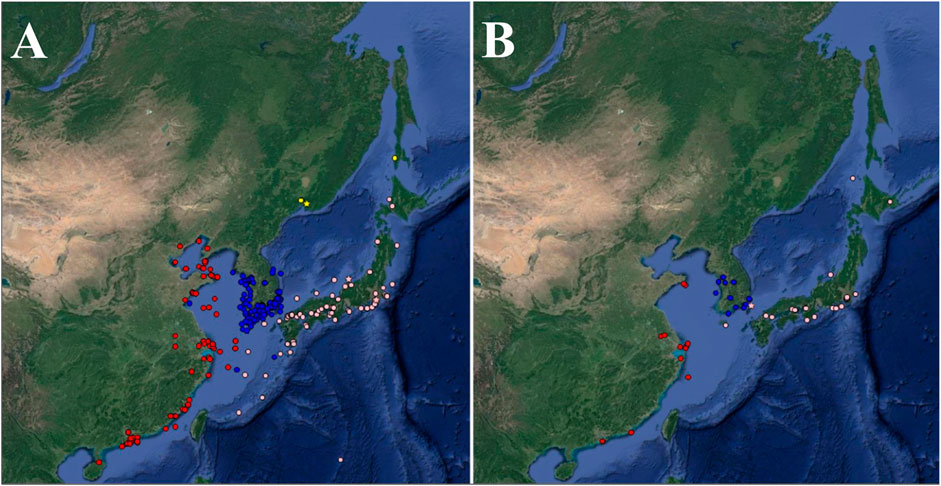
FIGURE 1. Spatial distribution of incident sites for (A) oil and (B) HNS spills greater than 10 tons in volume in the western North Pacific region. The stars represent the location of accidents that occurred in 2019 (blue: Korea, red: China, pink: Japan, yellow: Russia) (https://merrac.nowpap.org).

FIGURE 2

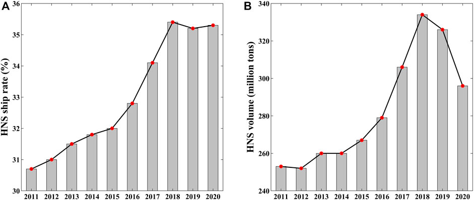
FIGURE 2. (A) Rate of arrival and departure of HNS cargo ships and (B) maritime transport volume of HNS in Korea from 2011 to 2020 (https://www.kmi.re.kr).

Because maritime HNS accidents usually occur in adverse weather conditions, such as strong winds, typhoons, and heavy rains, leaked HNS are highly likely to spread over a wide area in a short time owing to the ocean currents (Ceyhun, 2014). Highly toxic HNSs, such as benzene, toluene, and xylene, have serious adverse effects on the human body and various organisms living in marine ecosystems (Greenberg, 1997; Filley et al., 2004). Most colorless and transparent HNSs have limitations in visual identification and can cause secondary accidents because of explosions and fires, making human access difficult. To minimize the damage caused by an HNS spill accident that can lead to a large-scale disaster, a rapid and effective response strategy is required, and research in various fields pertaining to HNSs needs to be conducted.

Oil spill accidents are the main cause of the destruction of marine ecosystems, resulting in a high frequency of accidents and enormous damage. Numerous studies on oil spills have been conducted over a long period of time using various research methods and parameters, including diffusion models, spectral analysis, remote sensing, ecosystem impacts, risk assessment, and control strategies (Fingas and Brown, 2014; Duke, 2016; Spaulding, 2017; Chen et al., 2020; Viallefont-Robinet et al., 2021). Meanwhile, research on HNS is still at a basic stage because it is relatively new compared to the research on oil spills. Studies have focused on the construction of databases based on information on the behavior, fate, weathering and impacts of maritime HNS spills that have occurred worldwide (Cunha et al., 2015). In Korea, a spatial risk distribution map of the coast was presented based on a statistical analysis of HNS traffic volume and spill accidents (Lee and Jung, 2013). The HNS initial environmental risk assessment was introduced using the physicochemical properties, hazard, persistence, accumulation, emissions, and transport volume of HNS (Kim et al., 2019). Near-field propagation and metamodels have been analyzed to predict HNS spillage from ships, and a rapid toxicity evaluation method for HNS using shadow parameters for microalgae has also been developed (Ko et al., 2019; Seo et al., 2020). HNS has been detected using a faster region-based convolutional network in single-spectral ultraviolet images observed at a wavelength of 365 nm (Huang et al., 2020).

HNS remote sensing based on satellites and aircraft is effective in detecting HNS at sea because it has the advantage of monitoring a wide area and observing it at a high resolution. The HNS remote sensing project, PROOF improvement of HNS maritime POLLution by airborne radar and optical facilities, was conducted from 2014 to 2017 with the cooperation of several organizations, such as Office National d’Etudes et de Recherches Aérospatiales (ONERA), Centre of Documentation, Research and Experimentation on Accidental Water Pollution (CEDRE), Centre of Practical Expertise in Pollution Response, and Defence Research and Development Canada. In this campaign, HNSs were spilled into the Mediterranean Sea to perform aerial observations using hyperspectral and microwave synthetic aperture radar sensors (Angelliaume et al., 2017; Boisot et al., 2018).

To prepare for HNS spill accidents, it is important to not only detect the discharge area but also estimate the spill volume by calculating the thickness of the HNS floating in seawater. The thickness of oil can be roughly estimated according to color specifications such as silver, rainbow, metallic, transition dark, and dark colors, and it can also be estimated using the spectral reflectance measured from the satellite. A model for estimating oil film thickness based on the reflectance of near-infrared channels of the Moderate Resolution Imaging Spectro-radiometer and Medium Resolution Imaging Spectrometer has been proposed (Cox, 1954; De Carolis et al., 2013). Lu et al. (2012) introduced a quantitative theory between oil reflectance and thickness obtained via field experiments. In the case of mostly colorless HNSs, there is a limit to estimating the thickness visually; therefore, it is necessary to use the reflectance spectrum for thickness estimation. Recent research on the HNS spectra has focused on detection using a visible channel rather than the thickness; however, studies on HNS thickness estimation are infrequent (Park et al., 2021; Park et al., 2022). Therefore, this study aimed to (1) perform a ground hyperspectral spill experiment and acquire images assuming a marine HNS spill accident, (2) present the characteristics of radiance and reflectance in the shortwave infrared (SWIR) channel via spectral analysis, (3) estimate the toluene spill area by applying spectral mixture analysis, and (4) represent the spatial distribution of toluene thickness based on the two-beam interference model.

2 Data

2.1 Toluene spill experiment in a marine pool

Toluene is a colorless liquid that easily floats in water owing to its lower density and is classified as a volatile organic compound that evaporates easily (McCay et al., 2006; Diz Castro et al., 2015). In this study, we selected toluene as a representative HNS. Toluene ranks high in the HNS risk database, which is reflected in variables such as shipment volume, physicochemical properties, toxicity, persistence, bioaccumulation, and emissions (Kim et al., 2015). On land and in the coastal sea area around the Korean Peninsula, HNS spill accidents are caused by the collision and sinking of ships as well as by fires and explosions in industrial facilities located on the coast. A total of 24 toluene exposure incidents occurred, with spill volumes of up to 1 ton in some cases, from 2014 to 2021 (https://www.kmi.re.kr). The toluene spill experiment was first conducted to obtain spectral information regarding this substance on 2 September 2019, at the CEDRE’s marine pool in Brest, France. The length and width of the marine pool were 20 and 11 m, respectively. An Erlenmeyer flask with 1 L of toluene was attached to a long stick and poured inside a frame located at the center of the pool. After the spill, the diffused toluene was observed using a hyperspectral camera installed at a height of approximately 12 m (Figure 3A). The hyperspectral sensor was adjusted for observation at a perpendicular angle with the water surface, preventing sun glint effects. The effect of the sensor–zenith angle difference on the reflectance was negligible, with a maximum of 0.0035 at the farthest edge from the nadir, compared to the reflectance value at the nadir. Therefore, in this study, the differences in reflectance according to the zenith angle were not considered.

FIGURE 3

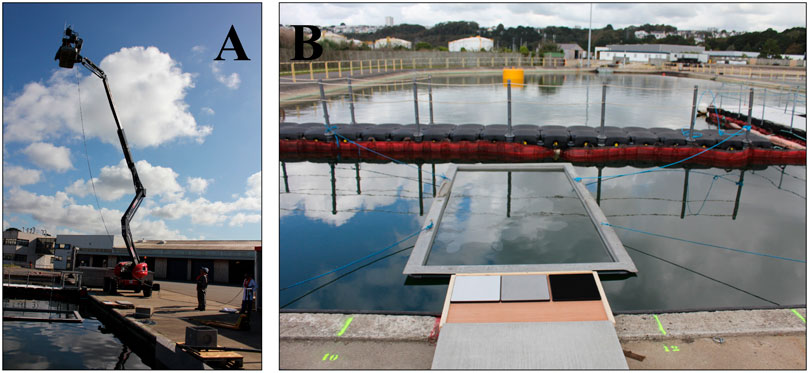
FIGURE 3. (A) Ground marine pool with a hyperspectral camera installed at a height of approximately 12 m. (B) Toluene spillage on the water surface.

Each hyperspectral camera of the visible and near-infrared (VNIR)-1600 and SWIR-1800 manufactured by HySpex was used by bonding. The VNIR-1600 sensor divides the wavelength range from 400 to 1,000 nm into 160 channels, and the SWIR-1800 sensor divides the wavelength range from 1,000 to 2,500 nm into 256 channels. At a height of 12 m, the spatial resolution of the SWIR sensor is 10.3 mm and 5.3 mm in the horizontal and vertical directions, respectively. Figure 3B shows an image taken with a digital single-lens reflection camera after the toluene spill showing transparent toluene with a circular shape. The frame was fastened using ropes to prevent movement. The white, gray, and black plates in the image are the reference targets for the reflectance conversion. The experiment was designed to ensure that all hyperspectral spectrum observations were obtained within 3 min of the toluene spill.

2.2 Spatial distribution of toluene RGB false color composite image

Hyperspectral toluene RGB (red: 997 nm, green: 1,238 nm, blue: 1,652 nm) false color composite images from the SWIR channel are shown in Figure 4A. Toluene and seawater can be identified in the RGB composite image with relatively high radiance in the visible channel (Park et al., 2021); however, composite images in the SWIR channel limit the classification of toluene in seawater because of its overall low radiance. The spatial distributions of the radiance of toluene and seawater were different at each RGB wavelength. At a wavelength of 997 nm, toluene and seawater pixels exhibited radiances of approximately 0.0010 and 0.0005, respectively (Figure 4B). Toluene and seawater pixels represent radiances of approximately 0.0005 and 0.0003, respectively, at a wavelength of 1,238 nm (Figure 4C). Toluene has a radiance of approximately 0.0002 at a wavelength of 1,652 nm (Figure 4D). In the RGB channel, the radiance of toluene and seawater, as well as the difference in radiance between the two substances, decreased as the wavelength increased.

FIGURE 4

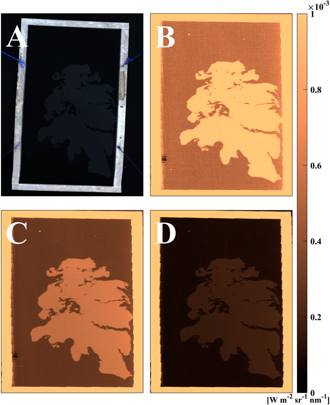
FIGURE 4. (A) Toluene RGB (red: 997 nm, green: 1,238 nm, blue: 1,652 nm) false color composite image observed with a hyperspectral SWIR sensor. Spatial distribution of toluene radiance in the (B) red, (C) green, and (D) blue channels.

3 Methods

3.1 Conversion of observed radiance to reflectance

The HNS raw data measured by the hyperspectral sensor were converted into radiance via radiometric correction provided by Norsk Elektro Optikk. In addition, reflectance conversion by atmospheric correction is required for HNS detection and thickness estimation. Empirical linear calibration based on vicarious radiometric calibration was used as an atmospheric correction method for hyperspectral images. It constructs a linear equation using the pixel value of a specific index, whose reflectance is known in advance and is applied to the total image. Eq. 1 is the relationship between radiance and reflectance, where the radiance ($L_s$) measured by the hyperspectral sensor is calculated as the product of the total downwelling radiance ($H$), reflectance ($\rho$), and atmospheric transmittance ($T$). Radiance is achieved by adding the atmospheric path radiance ($L_p$) to the product of three variables (Lavreau, 1991; Chavez, 1996; Song et al., 2001). Rectangular-shaped target plates with white (95%), gray (50%), and black (5%) reflectance were pre-positioned for inclusion in the hyperspectral image. $H\bullet T$ and $L_p$ are calculated from the average radiance and reflectance of the plate pixels in each channel; thus, toluene and seawater reflectance can be extracted at all wavelengths.

$L_s=H\bullet \rho \bullet T+L_p(1)$

3.2 Extraction of endmember spectra

HNS hyperspectral images obtained from the ground experiments were filled with pure toluene and seawater pixels, as well as mixtures of both substances. Spectral mixture analysis is a technique for extracting the spectra of pure substances that comprise hyperspectral images (Somers et al., 2011). Here, independent substances, such as toluene and seawater, are called endmembers. This method assumes that every pixel in the hyperspectral image consists of a linear mixture of endmembers, allowing the quantitative abundances of toluene and seawater to be compared at every pixel via both endmember spectra. Toluene and seawater endmember spectra were extracted using N-FINDR, a representative spectral mixture analysis method (Chang et al., 2010; Xiong et al., 2011). Assuming that the simplex composed of pure endmembers has the largest volume, the endmember representing the largest volume is extracted via training on randomly set p pixel combinations. In N-FINDR, the number of p endmembers is selected in advance, and the hyperspectral data are compressed into $p-1$ dimension via principal component analysis (Farrell and Mersereau, 2005). This method has the advantage of not requiring input variables other than the number of pure substances. The $p$ endmembers were calculated as the maximum volume ($V_{\mathit{max}}$) using Eq. 2. The volume of each simplex ($V_r$) is iteratively computed until the maximum volume is obtained by substituting all pixels ($r$) (Eq. 3).

$V_{\mathit{max}}=\frac{\left|\det \left[\begin{array}{c}1\\ e_1\end{array}\begin{array}{c}1\\ e_2\end{array}\begin{array}{c}\dots \\ \dots \end{array}\begin{array}{c}1\\ e_p\end{array}\right]\right|}{\left(p-1\right)!}(2)$

${V_r>V}_{\mathit{max}}(3)$

After extracting the representative endmember spectra of toluene and seawater, the abundance fraction ($\widehat{\alpha })$ occupied by each pixel is required. Eq. 4 represents the minimum reconstruction error ($e$) between the spectrum of the pixel vector ($r$) and the spectrum of the endmember ($M$) according to the abundance fraction. Heinz (2001) presented constraints that satisfy the abundance sum-to-one and non-negative constraints. Eqs 4, 5 represent the unconstrained least square (LS) and fully constrained least square (FCLS) solutions of the abundance fractions, where $I$ is a matrix of $p$ rows with elements 1. The hyperspectral toluene images in this study satisfy the FCLS.

$e={‖r-M\widehat{\alpha }‖}^2(4)$

${\widehat{\alpha }}_{LS}={\left(M^{T}M\right)}^{-1}{M}^{T}r(5)$

${\widehat{\alpha }}_{FCLS}={\widehat{\alpha }}_{LS}-{\left(M^{T}M\right)}^{-1}I*\left(I*{\left(M^{T}M\right)}^{-1}{I}^T\right)*\left(I^T*{\widehat{\alpha }}_{LS}-1\right)(6)$

3.3 HNS Gaussian mixture model

To improve toluene detection accuracy, it is important to select the optimal abundance fraction from seawater. In this study, a Gaussian mixture model (GMM)—a representative unsupervised learning method—was applied to the abundance fraction for all pixels assuming that both toluene and seawater abundance follow a Gaussian distribution. This model is useful when the data contain multiple Gaussian distributions. The GMM represents a normally distributed subpopulation within the entire population, and it is possible to automatically learn subpopulations without requiring data on subpopulations (Singh et al., 2009; Melnykov and Maitra, 2010). The types of values that parameterize the GMM are component weights, variances, and covariances (McLachlan et al., 2019). The probability distribution function of GMM is written as Eq. 7, where $x$ is the number of data points, and ${\mu }_k$ and ${\mathrm{\Sigma }}_k$ are the mean and covariance of the kth component, respectively. ${\pi }_k$ is defined as the weight of the mixture components and must be equal to 1. The probability distribution function of the D-dimensional Gaussian mixture is defined by Eq. 8. $\mu$ and $\mathrm{\Sigma }$ are the mean and Gaussian covariance matrices, respectively. Considering that the histogram of the abundance fraction corresponding to all pixels constituting the HNS image is composed of two peaks containing toluene and seawater rather than a single peak, the GMM is judged to be more suitable than a single model. The fraction with the lowest probability density between the two distributions was selected as the detection criterion.

$p\left(x\right)={\displaystyle \sum }_{k=1}^K{\pi }_{k}N\left(x\left|{\mu }_k\right.,{\sum }_k\right)(7)$

$P\left(x\left|\mu \right.,\sum \right)=\frac{1}{{\left(2\pi \right)}^{\frac{D}{2}}{\left|{\mathrm{\Sigma }}_k\right|}^{\frac{1}{2}}}\mathit{exp}\left(-\frac{1}{2}{\left(x-\mu \right)}^T{\mathrm{\Sigma }}^{-1}\left(x-\mu \right)\right)(8)$

3.3 HNS thickness estimation model

A two-beam interference theory model for oil thickness estimation was proposed by Lu et al. (2011) that is based on experiments measuring reflectance by increasing the amount of oil slick in seawater. In this model, the oil thickness was estimated based on the relationship between the reflectance and transmittance at the interface composed of three layers of air, oil, and seawater (Figure 5). The reflectance measured by the sensor consists of the ratio of the electric field strength $\stackrel{\rightharpoonup }{E_0}$ of sunlight to the sum of the reflected $\stackrel{\rightharpoonup }{E_1}$ and $\stackrel{\rightharpoonup }{E_2}$. $R_{12}$ and $T_{12}$ represent the reflectivity and transmissivity when incident from the atmosphere to the oil, respectively. $R_{23}$ is the reflectivity between the oil and seawater layers, and $T_{21}$ represents the transmissivity when incident from the oil to the atmosphere. $k$ and $\alpha$ denote the wavenumber and extinction coefficient of oil, respectively. $s$ is a variable for thickness $d$ and $\cos \theta$. Experiments were performed to determine the relationship between thickness and spectral reflectance using oil and seawater. Considering both zero and maximum oil thickness, an oil reflectance ($R$) model consisting of the maximum reflectance of oil ($R_{\mathit{max}}$), seawater reflectance $\left(R_{seawater}\right)$, $\alpha$, and thickness ($d)$ is suggested. In this study, the toluene reflectance spectrum was used instead of that of oil (Eq. 9). Toluene, an aromatic hydrocarbon (C-H), is a representative crude oil material in which one hydrogen atom occupying the benzene ring is substituted with a methyl group (-CH₃) (Moncayo-Riascos et al., 2020). It is similar to oil containing C-H compounds and exhibits an analogous reflectance tendency at SWIR wavelengths (Szwarc, 1948).

$R=R_{HNS-\mathit{max}}+\left(R_{seawater}-R_{HNS-\mathit{max}}\right)e^{-2\alpha d}(9)$

FIGURE 5

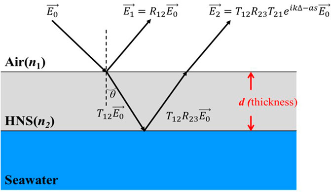
FIGURE 5. Schematic diagram of the two-beam interference model for offshore hazardous noxious substance (HNS) thickness estimation according to Lu et al. (2011).

3.4 Variation in toluene extinction coefficient

The toluene extinction coefficient was measured using a spectrophotometer (PerkinElmer Lambda 950), which covers a 400–2,500 nm wavelength range. The toluene thickness was classified into three cases: 0.2, 1, and 10 mm. As the extinction coefficient is independent of thickness, these three measurements were fitted using a model (Eq. 10) where $i$ is the thickness index and $T_i$ is the transmittance of the thickness $t{h}_i$. Variations in the toluene extinction coefficient from 400 to 1,750 nm are shown in Figure 6. In the wavelength range from 400 to 1,100 nm, the extinction coefficient has a value close to zero, indicating that toluene has little absorption of sunlight. However, the extinction coefficients of toluene at 1,140 nm and 1,380 nm were 0.1295 mm⁻¹ and 0.5777 mm⁻¹ with weak peaks. In the case of oil, it is known that the reflectance decreases at a wavelength of approximately 1,140 nm (Leifer et al., 2012). Contrastingly, toluene shows a higher response at wavelengths longer than 1,600 nm, indicated by a maximum peak of the extinction coefficient of approximately 1.3055 mm⁻¹ at 1,678 nm. The absorption of toluene primarily proceeds in the range of 1,600–1,700 nm; therefore, the SWIR channel is more suitable for measuring toluene thickness than the visible wavelength.

FIGURE 6

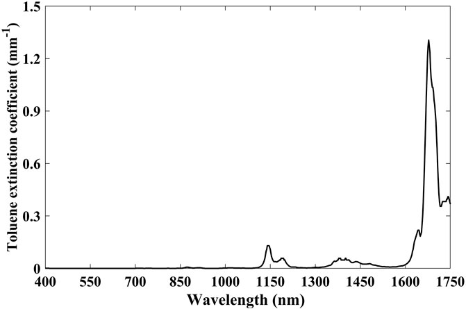
FIGURE 6. Variations in the toluene extinction coefficient as a function of wavelength.

The toluene reflectance spectrum in Figure 7B shows a marked decrease in the wavelength range from 1,650 to 1,700 nm, which is explained by the increasing trend in the toluene extinction coefficient. The trend of toluene reflectance in the SWIR channel is commonly observed for oils. The reflectance trend of deep-water horizontal oil decreases markedly at wavelengths of approximately 1,200 nm and 1,700 nm, known as the main spectral characteristic of C-H bonds (Leifer et al., 2012). In this study, toluene reflectance was utilized instead of oil reflectance in the thickness estimation model.

$T_i=e^{-\alpha \bullet t{h}_i}(10)$

FIGURE 7

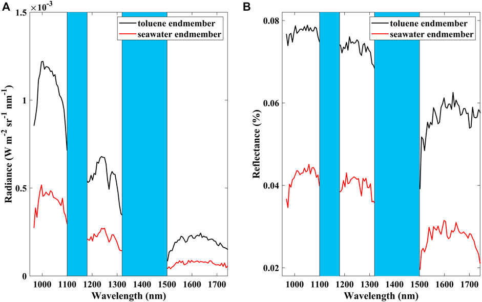
FIGURE 7. Comparison of toluene and seawater (A) radiance and (B) reflectance endmember spectra from shortwave infrared (SWIR) wavelength. The blue bars correspond to null transmission in the atmosphere.

4 Results

4.1 Endmember spectra of toluene

N-FINDR, a spectral mixing analysis, was applied to extract pure spectra representing HNS images. It was assumed that the hyperspectral image included toluene, seawater, and a mixture of the two substances, and the number of endmembers was set to two in advance. Figure 7A shows the variation in the radiance between the two endmembers at the SWIR wavelength extracted via N-FINDR. The black line with a relatively large radiance indicates toluene, and the red line represents seawater. Toluene tends to rapidly change its radiance at a wavelength of approximately 997 nm and shows a bimodal distribution with maximum radiances of 0.0007 and 0.0006 at 1,238 nm and 1,280 nm, respectively. It has an overall low radiance at wavelengths greater than 1,500 nm. Compared with toluene, the seawater endmember spectrum exhibited a relatively low radiance.

Toluene and seawater can be classified using quantitative differences in radiance (Park et al., 2021). As the purpose of this study is to estimate the thickness of toluene based on reflectance, two reflectance spectra were obtained by applying atmospheric correction to radiance in hyperspectral images (Figure 7B). The black and red lines represent toluene and seawater, respectively. Toluene has a reflectance of 0.078 at a wavelength of 1,003 nm, which remains relatively constant up to a wavelength of 1,100 nm. In particular, the reflectance gradually increased from 0.039 to 0.062 in the wavelength range of 1,500–1,650 nm but exhibited a tendency to markedly decrease to 0.053 at wavelength of 1,700 nm. This is in contrast to the rapid increase in the toluene extinction coefficient in a similar wavelength range, which is considered to be a relatively increased absorption rather than reflection at that wavelength. Seawater had a relatively low reflectance of 0.020–0.045 in the SWIR wavelength range. In the case of oil, its reflectance decreases at wavelengths near 1,730 nm owing to its C-H properties (Leifer et al., 2012). In contrast, the reflectance spectrum of toluene revealed a sharp decrease at approximately 1,680 nm, which was attributed to its C-H features. The toluene extinction coefficient also exhibited a sharp increase at a wavelength of approximately 1,680 nm. Thus, toluene showed a different reflectance characteristic than that of seawater.

4.2 Spatial distribution of the toluene abundance fraction

The spatial distribution of the abundance fractions was determined from the reflectance endmember spectra of toluene and seawater. The fraction must have a positive value, and the sum of the fractions of the two endmembers in every pixel must satisfy 100% (Heinz, 2001). In the abundance fraction map for the toluene endmember (Figure 8A), red pixels with a ratio greater than 60% represent toluene, and blue pixels with a ratio of less than 20% correspond to seawater. Toluene is primarily located in the center and is surrounded by seawater. Pixels close to 100% indicate pure toluene endmembers, whereas violet pixels close to 0% are considered pure seawater spectra.

FIGURE 8

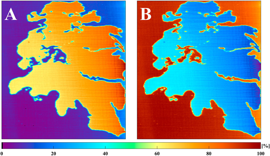
FIGURE 8. Spatial distribution of (A) toluene and (B) seawater abundance fraction maps from endmember spectra in shortwave infrared wavelengths.

The proportion of toluene pixels distributed on the right side of the image was greater than 80%, whereas the proportion of pixels located on the left side was between 60% and 80%. Pixels with a ratio lower than 10% are distributed in the center of toluene, which is considered to be occupied by seawater because it is splashed during the process of pouring toluene. From the center of the toluene to the boundary, the proportion of pixels decreased sharply by approximately 40%. This indicates that pixels with a mixture of toluene and seawater existed. The abundance fraction of the seawater endmember was opposite to that of the toluene endmember (Figure 8B). The fraction of most toluene pixels was less than 40%, whereas the ratio of the surrounding seawater pixels was greater than 80%.

4.3 Classification of toluene and seawater pixels

It is important to select the optimal abundance fraction threshold for the classification of toluene and seawater. The probability density of toluene occupancy for all pixels was expressed via a histogram analysis. The probability densities of the toluene and seawater pixels were represented as multimodal distributions at 72% and 8% ratios, respectively. Most of the toluene and seawater fractions appeared in the ranges of 63–81% and 3–9%, respectively (Figure 9A). The boundary pixels of the two substances are in the range of 30–60%, and the minimum density of the curve fit was close to zero at a 36% fraction. Therefore, a ratio of 36% was selected as the criterion to distinguish between toluene and seawater.

FIGURE 9

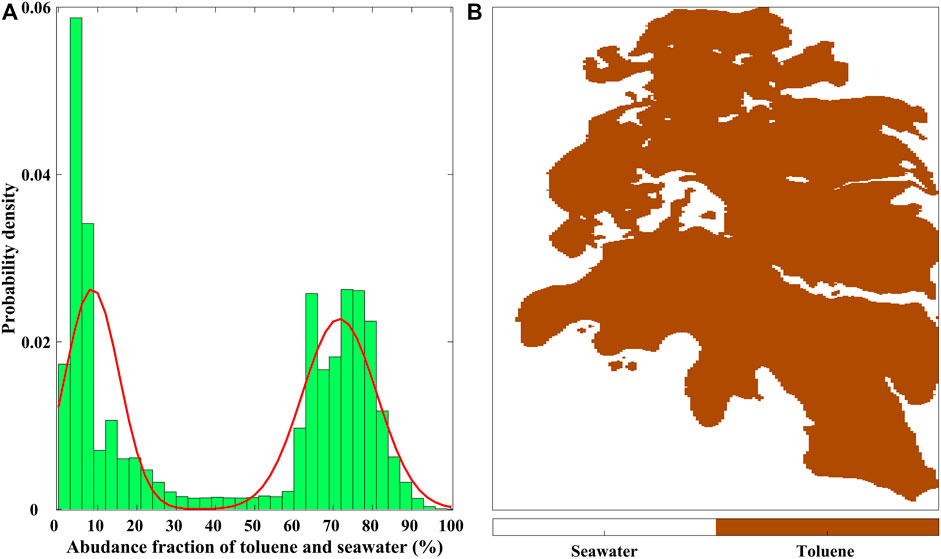
FIGURE 9. (A) Histogram of probability density distribution based on the abundance fraction of toluene endmember spectra and (B) spatial distribution of classification result of toluene and seawater (<36%).

The spatial distributions of toluene and seawater, according to the abundance fraction at 36%, are shown in Figure 9B. The total number of pixels detected with toluene was 44,544, accounting for 54.11% of the image. Considering the spatial resolution of the hyperspectral image, the extent of the toluene spill was estimated to be approximately 2.4317 m². Assuming that 1 L of toluene used in the experiment is 100% floating, the average thickness of the detected toluene pixels is 0.4112 mm. However, because toluene floats on water and is volatile, it is expected that there will be some errors because of its evaporation or partial dissolution after spillage.

4.4 Spatial distribution of toluene thickness

Toluene thickness was estimated using toluene reflectance at 1,676.5 nm closest to the wavelength showing the maximum extinction coefficient. Figure 10A shows the spatial distribution of toluene and seawater reflectance at 1,676.5 nm. Applying the 36% abundance fraction as the toluene detection criterion to the image, the average and maximum toluene reflectance were 0.0493 and 0.0605, respectively. The average reflectance of seawater was 0.0316. Figure 10B shows the spatial distribution of the toluene thickness estimated using the two-beam interference thickness model. The average and maximum thicknesses in the images were 0.3839 mm and 2.0854 mm, respectively. The toluene pixels located on the right side rather than the left side of the image are relatively thick, which is similar to the spatial distribution of the toluene abundance fraction. Assuming that 1 L of toluene is only floating in seawater, the average thickness should be 0.4112 mm; however, the average thickness estimated in this study is approximately 0.3839 mm. The total volume of toluene calculated using spectral mixture analysis and thickness model was approximately 0.9336 L. This error is approximately 6.64% of the actual amount of toluene spilled.

FIGURE 10

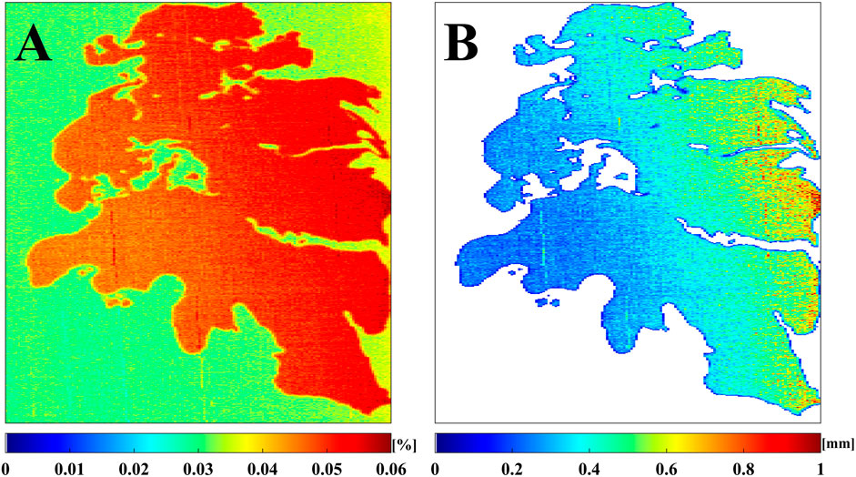
FIGURE 10. Spatial distribution of (A) toluene reflectance at 1,676.5 nm wavelength and (B) estimated thickness.

5 Discussion and conclusion

Toluene is a colorless organic compound that floats in water owing to its low density and evaporates easily. Absorption of toluene into the human body upon breathing or skin exposure for a long time exerts adverse effects on the nervous system, such as headaches, dizziness, memory loss, and hallucinations (Saito and Wada, 1993). Such an HNS leakage accident is highly likely to occur anywhere in the world, not just in the Korean Peninsula. From 2002 to 2021, 20 incidents of toluene exposure have occurred consistently, as reported by the Department of Labor, Occupational Safety and Health Administration of the United States. Unlike oil, HNSs floating in seawater are exceedingly difficult to detect visually; therefore, satellite and aircraft-based HNS remote sensing approaches are needed. In this study, a ground hyperspectral HNS spill experiment was performed as a basic study for maritime HNS detection. After spilling 1 L of toluene into an outdoor marine pool, it was observed using a hyperspectral sensor with SWIR wavelengths. To detect toluene, a spectral mixing technique was applied to the images obtained from the experiment, and the thickness was estimated using a two-beam interference model.

Although we precisely designed and constructed the HNS spill experiment and retrieved the actual amount of spill material with reasonable results, there are many factors that could affect the estimation of HNS thickness in the complex marine environment. One of the most important factors may be wind speed, which controls the evaporation of HNSs and their rapid mixing with the sea water. The effect of the wind field on thickness estimation should be further investigated based on more intensive experiments in both marine pools and a real sea environment. In this study, the estimated total toluene volume was slightly reduced compared with the amount of toluene spilled in the experiment. As the elapsed time from the toluene leak to the observation with the hyperspectral sensor is up to 3 min, this is unlikely; however, there is a slight possibility that the toluene may evaporate into the air or dissolve into the water. In addition to the effect of wind speed, the evaporation of toluene is affected by other atmospheric and marine conditions, such as air temperature, humidity, the temperature difference between the air and sea surface temperatures, and the sea state, including various waves.

Even though we conducted the HNS experiment under calm atmospheric conditions, its evaporation could potentially contribute to errors. To verify the evaporation of HNSs, it is necessary to consider the brightness temperature difference at the LWIR wavelength (Foucher et al., 2016). In the case of aromatic substances, including toluene, xylene, and benzene, they are known to form a cold slick via endothermic reaction after a spill. Conversely, for alcohol substances such as methanol and propanol, the slick is measured at high temperatures via an exothermic reaction. Further, there are two approaches to the quantitative analysis of gas plumes (Foucher and Doz, 2019). The first is an endmember decomposition technique to estimate background properties and detect trace elements (Funk et al., 2001). The second method is based on the estimation of all radiative terms, including background, atmospheric condition, and gas species. Most quantitative algorithms aim to estimate ground and gas properties using iterative minimization between radiative transfer model calculations and measurements (Gafalk et al., 2016; Kuai et al., 2016). In this study, we tried to minimize the effect of evaporation by performing immediate and simultaneous observation with a hyperspectral sensor after spillage. Although specific environmental information was not monitored in the experiment, the ECMWF Reanalysis v5 data showed that the air temperature, evaporation rate, and wind speed were 18.176°C, 0.243 mm day⁻¹, and 2.053 m s⁻¹ respectively, at approximately 12:30 p.m. local time in the study area. These weak winds are expected to have caused little evaporation. In future studies, a more detailed experiment design, including atmospheric measurements, and a more accurate model for toluene thickness estimation will be necessary.

It is possible that there was an error in the toluene and seawater boundary pixels. Toluene and seawater were classified on the basis of the minimum probability density of the toluene abundance fraction. Most of the pixels affected by the toluene endmember spectrum were classified as toluene; however, some toluene pixels near the threshold were considered as seawater. In addition, as the two-beam interference theory for thickness estimation is based on oil reflectance, toluene may have limitations that were not considered in the model equation of this study, which focused on the reflectance spectrum trend of the two materials at the SWIR wavelength. When toluene and oil emulsification occurred, a decrease in reflectance was commonly observed at wavelengths ranging 1,600–1,700 nm owing to the chemical properties associated with the C-H bonds.

Although some studies on HNS detection using remote sensing have been introduced, a model for quantitative HNS thickness estimation has not yet been proposed. Even though the two-beam model represents a reasonable HNS thickness, additional experiments should be performed on an upper limit of HNS thickness under controlled conditions in the future. Considering these limitations, this study evaluated the applicability of HNS detection and thickness estimation based on oil-like reflectance spectral trends at SWIR wavelengths. Despite the various limitations and potential interfering factors of this approach, this study is meaningful in the field of HNS monitoring as it is the first attempt to detect toluene and estimate its thickness based on hyperspectral remote sensing. Therefore, this study is expected to be helpful for marine HNS accident monitoring and harmful marine ecosystem environment evaluation.

Data availability statement

The datasets presented in this article are not readily available because data can be shared only through collaboration between scientists with non-commercial purposes. Requests to access the datasets should be directed to a2FwYXJrQHNudS5hYy5rcg==.

Author contributions

Conceptualization, K-AP; data processing, P-YF and J-JP; methodology, K-AP and J-JP; writing—original draft preparation, J-JP; writing—review and editing, K-AP; discussion and funding, T-SK and ML. All authors contributed to the final version of the manuscript.

Funding

This study was supported by the National Research Foundation of Korea (NRF), grant funded by the Korean government (MSIT) (No. 2020R1A2C2009464). The first author was partly supported by the Korea Institute of Marine Science and Technology Promotion (KIMST) and funded by the Ministry of Oceans and Fisheries, Republic of Korea (20210660).

Conflict of interest

The authors declare that the research was conducted in the absence of any commercial or financial relationships that could be construed as a potential conflict of interest.

Publisher’s note

All claims expressed in this article are solely those of the authors and do not necessarily represent those of their affiliated organizations, or those of the publisher, the editors and the reviewers. Any product that may be evaluated in this article, or claim that may be made by its manufacturer, is not guaranteed or endorsed by the publisher.

References

Angelliaume, S., Minchew, B., Chataing, S., Martineau, P., and Miegebielle, V. (2017). Multifrequency radar imagery and characterization of hazardous and noxious substances at sea. IEEE Trans. Geosci. Remote Sens. 55 (5), 3051–3066. doi:10.1109/tgrs.2017.2661325

CrossRef Full Text | Google Scholar

Boisot, O., Angelliaume, S., and Guérin, C. A. (2018). Marine oil slicks quantification from L-band dual-polarization SAR imagery. IEEE Trans. Geosci. Remote Sens. 57 (4), 2187–2197. doi:10.1109/tgrs.2018.2872080

CrossRef Full Text | Google Scholar

Ceyhun, G. C. (2014). The impact of shipping accidents on marine environment: A study of Turkish seas. Eur. Sci. J. 10 (23), 10–23. doi:10.19044/esj.2014.v10n23p%25p

CrossRef Full Text | Google Scholar

Chang, C. I., Wu, C. C., and Tsai, C. T. (2010). Random N-finder (N-FINDR) endmember extraction algorithms for hyperspectral imagery. IEEE Trans. Image Process 20 (3), 641–656. doi:10.1109/TIP.2010.2071310

PubMed Abstract | CrossRef Full Text | Google Scholar

Chavez, P. S. (1996). Image-based atmospheric corrections-revisited and improved. Photogramm. Eng. Remote Sens. 62 (9), 1025–1035.

Google Scholar

Chen, J., Di, Z., Shi, J., Shu, Y., Wan, Z., Song, L., et al. (2020). Marine oil spill pollution causes and governance: A case study of sanchi tanker collision and explosion. J. Clean. Prod. 273, 122978. doi:10.1016/j.jclepro.2020.122978

CrossRef Full Text | Google Scholar

Chen, J., Zhang, W., Wan, Z., Li, S., Huang, T., and Fei, Y. (2019). Oil spills from global tankers: Status review and future governance. J. Clean. Prod. 227, 20–32. doi:10.1016/j.jclepro.2019.04.020

CrossRef Full Text | Google Scholar

Cho, S. J., Kim, D. J., and Choi, K. S. (2013). Hazardous and noxious substances (HNS) risk assessment and accident prevention measures on domestic marine transportation. J. Korean Soc. Mar. 19 (2), 145–154. doi:10.7837/kosomes.2013.19.2.145

CrossRef Full Text | Google Scholar

Cox, C. (1954). Statistics of the sea surface derived from sun glitter. J. Mar. Res. 13, 198–227.

Google Scholar

Cunha, I., Moreira, S., and Santos, M. M. (2015). Review on hazardous and noxious substances (HNS) involved in marine spill incidents—an online database. J. Hazard. Mat. 285, 509–516. doi:10.1016/j.jhazmat.2014.11.005

PubMed Abstract | CrossRef Full Text | Google Scholar

De Carolis, G., Adamo, M., and Pasquariello, G. (2013). On the estimation of thickness of marine oil slicks from sun-glittered, near-infrared MERIS and MODIS imagery: The Lebanon oil spill case study. IEEE Trans. Geosci. Remote Sens. 52 (1), 559–573. doi:10.1109/tgrs.2013.2242476

CrossRef Full Text | Google Scholar

Diz Castro, M., Gómez-Díaz, D., Amrane, A., and Couvert, A. (2015). Toluene biodegradation in a solid/liquid system involving immobilized activated sludge and silicone oil as pollutant reservoir. Environ. Technol. 36 (4), 450–454. doi:10.1080/09593330.2014.951402

PubMed Abstract | CrossRef Full Text | Google Scholar

Duke, N. C. (2016). Oil spill impacts on mangroves: Recommendations for operational planning and action based on a global review. Mar. Pollut. Bull. 109 (2), 700–715. doi:10.1016/j.marpolbul.2016.06.082

PubMed Abstract | CrossRef Full Text | Google Scholar

Farrell, M. D., and Mersereau, R. M. (2005). On the impact of PCA dimension reduction for hyperspectral detection of difficult targets. IEEE Geosci. Remote Sens. Lett. 2 (2), 192–195. doi:10.1109/lgrs.2005.846011

CrossRef Full Text | Google Scholar

Filley, C. M., Halliday, W., and Kleinschmidt-DeMasters, B. K. (2004). The effects of toluene on the central nervous system. J. Neuropathol. Exp. Neurol. 63 (1), 1–12. doi:10.1093/jnen/63.1.1

PubMed Abstract | CrossRef Full Text | Google Scholar

Fingas, M., and Brown, C. (2014). Review of oil spill remote sensing. Mar. Pollut. Bull. 83 (1), 9–23. doi:10.1016/j.marpolbul.2014.03.059

PubMed Abstract | CrossRef Full Text | Google Scholar

Foucher, P. Y., and Doz, S. (2019). Real time gas quantification using thermal hyperspectral imaging: Ground and airborne applications. STO-MP-SET-277-18. NATO’s Science and Technology Organization.

Google Scholar

Foucher, P. Y., Poutier, L., Déliot, P., Puckrin, E., and Chataing, S. (2016). “Hazardous and Noxious Substance detection by hyperspectral imagery for marine pollution application,” in Proceedings of the IGARSS 2016 - 2016 IEEE International Geoscience and Remote Sensing Symposium, 10-15 July 2016, Beijing, China (IEEE), 7694–7697.

CrossRef Full Text | Google Scholar

Funk, C. C., Theiler, J., Roberts, D. A., and Borel, C. C. (2001). Clustering to improve matched filter detection of weak gas plumes in hyperspectral thermal imagery. IEEE Trans. Geosci. Remote Sens. 39 (7), 1410–1420. doi:10.1109/36.934073

CrossRef Full Text | Google Scholar

Gafalk, M., Olofsson, G., Crill, P., and Bastviken, D. (2016). Making methane visible. Nat. Clim. Change 6, 426–430. doi:10.1038/nclimate2877

CrossRef Full Text | Google Scholar

Greenberg, M. M. (1997). The central nervous system and exposure to toluene: A risk characterization. Environ. Res. 72 (1), 1–7. doi:10.1006/enrs.1996.3686

PubMed Abstract | CrossRef Full Text | Google Scholar

Harold, P. D., De Souza, A. S., Louchart, P., Russell, D., and Brunt, H. (2014). Development of a risk-based prioritisation methodology to inform public health emergency planning and preparedness in case of accidental spill at sea of hazardous and noxious substances (HNS). Environ. Int. 72, 157–163. doi:10.1016/j.envint.2014.05.012

PubMed Abstract | CrossRef Full Text | Google Scholar

Heinz, D. C., and Chein-I-Chang, (2001). Fully constrained least squares linear spectral mixture analysis method for material quantification in hyperspectral imagery. IEEE Trans. Geosci. Remote Sens. 39 (3), 529–545. doi:10.1109/36.911111

CrossRef Full Text | Google Scholar

Huang, H., Wang, C., Liu, S., Sun, Z., Zhang, D., Liu, C., et al. (2020). Single spectral imagery and faster R-CNN to identify hazardous and noxious substances spills. Environ. Pollut. 258, 113688. doi:10.1016/j.envpol.2019.113688

PubMed Abstract | CrossRef Full Text | Google Scholar

Kim, Y. R., Kim, T. W., Son, M. H., Oh, S., and Lee, M. (2015). A study on prioritization of HNS management in Korean waters. J. Korean Soc. Mar. Environ. Saf. 21 (6), 672–678. doi:10.7837/kosomes.2015.21.6.672

CrossRef Full Text | Google Scholar

Kim, Y. R., Lee, M., Jung, J. Y., Kim, T. W., and Kim, D. (2019). Initial environmental risk assessment of hazardous and noxious substances (HNS) spill accidents to mitigate its damages. Mar. Pollut. Bull. 139, 205–213. doi:10.1016/j.marpolbul.2018.12.044

PubMed Abstract | CrossRef Full Text | Google Scholar

Ko, M. K., Jeong, C. H., Lee, M., and Lee, S. H. (2019). Development of a metamodel for predicting near-field propagation of hazardous and noxious substances spilled from a ship. Appl. Sci. 9 (18), 3838, doi:10.3390/app9183838

CrossRef Full Text | Google Scholar

Kuai, F. L., Worden, J. R., Li, K. F., Hulley, G. C., Hopkins, F. M., Miller, C. E., et al. (2016). Characterization of anthropogenic methane plumes with the hyperspectral thermal emission spectrometer (HyTES): A retrieval method and error analysis. Atmos. Meas. Tech. 9, 3165– 3173. doi:10.5194/amt-9-3165-2016

CrossRef Full Text | Google Scholar

Lavreau, J. (1991). De-hazing Landsat thematic mapper images. Photogramm. Eng. Remote Sens. 57 (10), 1297–1302.

Google Scholar

Lee, M., and Jung, J. Y. (2013). Risk assessment and national measure plan for oil and HNS spill accidents near Korea. Mar. Pollut. Bull. 73 (1), 339–344. doi:10.1016/j.marpolbul.2013.05.021

PubMed Abstract | CrossRef Full Text | Google Scholar

Leifer, I., Lehr, W. J., Simecek-Beatty, D., Bradley, E., Clark, R., Dennison, P., et al. (2012). State of the art satellite and airborne marine oil spill remote sensing: Application to the BP Deepwater Horizon oil spill. Remote Sens. Environ. 124, 185–209. doi:10.1016/j.rse.2012.03.024

CrossRef Full Text | Google Scholar

Lu, Y., Li, X., Tian, Q., and Han, W. (2012). An optical remote sensing model for estimating oil slick thickness based on two-beam interference theory. Opt. Express 20 (22), 24496–24504. doi:10.1364/oe.20.024496

PubMed Abstract | CrossRef Full Text | Google Scholar

Lu, Y., Tian, Q., and Li, X. (2011). The remote sensing inversion theory of offshore oil slick thickness based on a two-beam interference model. Sci 54 (5), 678–685. doi:10.1007/s11430-010-4154-1

CrossRef Full Text | Google Scholar

McCay, D. P. F., Whittier, N., Ward, M., and Santos, C. (2006). Spill hazard evaluation for chemicals shipped in bulk using modeling. Environ. Model. Softw. 21 (2), 156–169. doi:10.1016/j.envsoft.2004.04.021

CrossRef Full Text | Google Scholar

McLachlan, G. J., Lee, S. X., and Rathnayake, S. I. (2019). Finite mixture models. Annu. Rev. Stat. Appl. 6, 355–378. doi:10.1146/annurev-statistics-031017-100325

CrossRef Full Text | Google Scholar

Melnykov, V., and Maitra, R. (2010). Finite mixture models and model-based clustering. Stat. Surv. 4, 80–116. doi:10.1214/09-ss053

CrossRef Full Text | Google Scholar

Michail, N. A., and Melas, K. D. (2020). Shipping markets in turmoil: An analysis of the Covid-19 outbreak and its implications. Transp. Res. Interdiscip. Perspect. 7, 100178. doi:10.1016/j.trip.2020.100178

PubMed Abstract | CrossRef Full Text | Google Scholar

Moncayo-Riascos, I., Taborda, E., Hoyos, B. A., Franco, C. A., and Cortés, F. B. (2020). Theoretical-experimental evaluation of rheological behavior of asphaltene solutions in toluene and p-xylene: Effect of the additional methyl group. J. Mol. Liq. 303, 112664. doi:10.1016/j.molliq.2020.112664

CrossRef Full Text | Google Scholar

Neuparth, T., Moreira, S., Santos, M. M., and Reis-Henriques, M. A. (2011). Hazardous and noxious substances (HNS) in the marine environment: Prioritizing HNS that pose major risk in a European context. Mar. Pollut. Bull. 62 (1), 21–28. doi:10.1016/j.marpolbul.2010.09.016

PubMed Abstract | CrossRef Full Text | Google Scholar

Park, J. J., Park, K., Foucher, P. Y., Deliot, P., Floch, S. L., Kim, T. S., et al. (2021). Hazardous noxious substance detection based on ground experiment and hyperspectral remote sensing. Remote Sens. 13 (2), 318. doi:10.3390/rs13020318

CrossRef Full Text | Google Scholar

Park, J. J., Park, K., Kim, T. S., and Lee, M. (2022). Hazardous and noxious substances (HNSs) styrene detection using spectral matching and mixture analysis methods. J. Korean Soc. Mar. Environ. Saf. 28 (S), 1–10. doi:10.7837/kosomes.2022.28.s.001

CrossRef Full Text | Google Scholar

Saito, K., and Wada, H. (1993). Behavioral approaches to toluene intoxication. Environ. Res. 62 (1), 53–62. doi:10.1006/enrs.1993.1088

PubMed Abstract | CrossRef Full Text | Google Scholar

Seo, D., Shin, S., Oh, S., Lee, M., and Seo, S. (2020). Rapid eco-toxicity analysis of hazardous and noxious substances (HNS) using morphological change detection in Dunaliella tertiolecta. Algal Res. 51, 102063. doi:10.1016/j.algal.2020.102063

CrossRef Full Text | Google Scholar

Singh, R., Pal, B. C., and Jabr, R. A. (2009). Statistical representation of distribution system loads using Gaussian mixture model. IEEE Trans. Power Syst. 25 (1), 29–37. doi:10.1109/tpwrs.2009.2030271

CrossRef Full Text | Google Scholar

Somers, B., Asner, G. P., Tits, L., and Coppin, P. (2011). Endmember variability in spectral mixture analysis: A review. Remote Sens. Environ. 115 (7), 1603–1616. doi:10.1016/j.rse.2011.03.003

CrossRef Full Text | Google Scholar

Song, C., Woodcock, C. E., Seto, K. C., Lenney, M. P., and Macomber, S. A. (2001). Classification and change detection using landsat TM data: When and how to correct atmospheric effects? Remote Sens. Environ. 75 (2), 230–244. doi:10.1016/s0034-4257(00)00169-3

CrossRef Full Text | Google Scholar

Spaulding, M. L. (2017). State of the art review and future directions in oil spill modeling. Mar. Pollut. Bull. 115 (1–2), 7–19. doi:10.1016/j.marpolbul.2017.01.001

PubMed Abstract | CrossRef Full Text | Google Scholar

Szwarc, M. (1948). The C–H bond energy in toluene and xylenes. J. Chem. Phys. 16 (2), 128–136. doi:10.1063/1.1746794

CrossRef Full Text | Google Scholar

Viallefont-Robinet, F., Roupioz, L., Caillault, K., and Foucher, P. Y. (2021). Remote sensing of marine oil slicks with hyperspectral camera and an extended database. J. Appl. Remote Sens. 15 (2), 024504. doi:10.1117/1.jrs.15.024504

CrossRef Full Text | Google Scholar

Xiong, W., Chang, C. I., Wu, C. C., Kalpakis, K., and Chen, H. M. (2011). Fast algorithms to implement N-FINDR for hyperspectral endmember extraction. IEEE J. Sel. Top. Appl. Earth Obs. Remote Sens. 4 (3), 545–564. doi:10.1109/jstars.2011.2119466

CrossRef Full Text | Google Scholar