 Xiaolong Jin
 Xueliang Deng
 Jian Chen1
94% of researchers rate our articles as excellent or good
Learn more about the work of our research integrity team to safeguard the quality of each article we publish.
Find out more
ORIGINAL RESEARCH article
Front. Environ. Sci., 17 March 2023
Sec. Atmosphere and Climate
Volume 11 - 2023 | https://doi.org/10.3389/fenvs.2023.1129639
This article is part of the Research TopicClimate-Environment Interactions under Global WarmingView all 25 articles
With the improved accuracy and high spatiotemporal resolution, satellite remote sensing has provided an alternative way for monitoring the variations of CO2 in remote areas where field observations are inadequately sampled but the emissions of CO2 are increasing rapidly. Based on CO2 estimates from satellite remote sensing and the atmospheric tracer transport model, this study assessed the spatiotemporal patterns of atmospheric CO2 and its driving forces across China. Results show a consistent increase in CO2 at all levels of the troposphere, with the growth rate exceeding 2.1 ppm/year. Among them, the near surface witnessed obvious spatial heterogeneity with the highest concentrations of CO2 occurring in East China and the lowest in Northwest China. This strong spatial differentiation disappeared with increase in altitude and is replaced by a distinct south–north gradient difference at the upper troposphere. With regard to vertical variations, the concentration and growth rates of CO2 at the lower troposphere are generally higher than those at the upper troposphere. The driving mechanism analysis indicates that the variation of CO2 at the near surface is primarily caused by anthropogenic and biogenic activities, while air motion dominates the distribution of CO2 at the upper troposphere. The findings of the present study could provide a valuable reference for understanding regional carbon cycles and formulating carbon emission reduction strategies on a national scale.
Carbon dioxide (CO2) is the main greenhouse gas causing global warming. It contributes more than 60% of the total radiative forcing and has a lifespan of more than 120 years in the atmosphere (Stocker et al., 2013). Due to massive fossil fuel combustion and dramatic land use changes, the level of global average atmospheric CO2 has increased by 140% relative to pre-industrial levels and reached 414.72 ppm in 2021 (Peters et al., 2011; WMO, 2012). The increasing concentrations of CO2 have led to a positive energy imbalance of 0.53 ± 0.11 W/m2 from 2003 to 2018, causing an increase in atmospheric temperature and sea level (Kramer et al., 2021), which in turn led to a series of meteorological disasters such as the melting of polar glaciers and frequent drought and flood events (IPCC, 2014). The continuous increase in the concentration of atmospheric CO2 has attracted a significant attention from the international community and organizations. Accurately and comprehensively assessing the spatial and temporal distribution of atmospheric CO2 can provide a foundation for understanding the global carbon cycle and will aid in the formulation of policies aimed at reducing carbon emissions (Umezawa et al., 2018).
For this purpose, the long-term measurement of atmospheric CO2 concentrations in different regions of the world has been established and gradually evolved into a global network of CO2 observation. Currently, there are more than 300 sites worldwide, where greenhouse gas levels are measured by the World Meteorological Organization/Global Atmosphere Watch (WMO/GAW) (WMO, 2012; Fang et al., 2014). The integrated carbon observation system provides a reliable dataset for assessing long-term changes of atmospheric CO2 at the global and regional scales and plays an important role in the early research on carbon sources and sinks. However, restricted to the level of socioeconomic development and topographic factors, the GAW ground-based observations are sparse and unevenly distributed, with most of them located in developed countries or plain areas (Mustafa et al., 2020). In addition, the discontinuities and inconsistencies in multi-sources of observational data further complicate the availability of data, making the spatiotemporal distribution studies of atmospheric CO2 uncertain and challenging (Fang et al., 2014; Basu et al., 2013).
The development of satellite remote sensing technology has provided an alternative method for monitoring the spatiotemporal distribution of CO2 on a global scale. By combining various satellite sensors and high-precision inversion algorithms, CO2 products are generated based on the characteristics of its absorption spectrum at the thermal and near-infrared bands (Schneising, 2008). To date, three satellite projects dedicated to CO2 observation have been launched, i.e., the Greenhouse Gases Observing Satellite (GOSAT) (Yokota et al., 2009), the Orbiting Carbon Observatory (OCO) (Crisp, 2015), and the Chinese carbon dioxide observation satellite mission (TanSat) (Liu et al., 2018). Compared with the field observation, satellite CO2 estimates are not subject to topographical factors and can achieve a stable and continuous observation of atmospheric CO2 at the regional and global scales with high spatiotemporal resolution (Zeng et al., 2013). With a large spatial coverage from near surface to the troposphere and a long temporal period (2009–present), the GOSAT has been widely applied in research studies of carbon sources and sinks and the transport of atmospheric CO2 (Basu et al., 2013; Mustafa et al., 2020). In general, the progressive development of space-borne sensors and inversion algorithms has made satellite remote sensing the main method of monitoring atmospheric CO2 variations and has enhanced our understanding of regional and global carbon cycles.
By integrating ground-based and satellite remote sensing observation data, numerous studies have been conducted to explore the spatiotemporal differentiation of CO2 and the associated driving forces (Cao et al., 2019; Kong et al., 2019; Yang et al., 2021). However, most of the studies focused on Western Europe and the United States. Northeastern Asia, a densely populated region with high CO2 emissions, has not been adequately explored. As a matter of fact, China has witnessed rapid economic development over the last three decades, and the rapid increase in fossil fuel carbon emissions has made China the leading contributor of global CO2 emissions (Le Quéré et al., 2012; Du et al., 2017). In this regard, China has implemented a number of programs aimed at reducing carbon emissions and conserving energy and has committed to achieving carbon peak by 2030 and carbon neutrality by 2060. Therefore, it is important to evaluate the spatiotemporal variation of CO2 and explore the driving mechanism, as this could provide valuable information for understanding the carbon cycle and constraining carbon emissions on a national scale (Hammerling et al., 2012; Fang et al., 2014).
To assess the characteristics of CO2 variations and investigate its driving forces on a national scale, we chose a fast-economic growth and high carbon emission area, i.e., China, as the study region and obtained CO2 estimates from satellite remote sensing (GOSAT) and an atmospheric tracer transport model (Carbon Tracker). Meanwhile, the data of leaf area index (LAI), fossil fuel carbon emissions, and the 3D wind field were also collected. In particular, we aimed to (1) analyze the spatial and temporal variation of CO2 at different time scales across China, (2) explore the dominant factors affecting the regional concentrations of CO2, and (3) examine the relationship between local CO2 and LAI, fossil fuel carbon emissions, and regional air motion.
As one of the largest countries in the world, China covers a vast territory (9.6 × 10⁶ km2) with heterogeneities in climatic conditions, complex topographies, and ecological environments, which have caused strong variations in economic development and population growth. A combination of climatic diversity and human activity has resulted in a unique pattern of local carbon budgets with obvious spatial differences in CO2 concentrations (Fang et al., 2014; Du et al., 2017). To address this issue, six sub-regions characterized by different climatic conditions and socioeconomic backgrounds were delineated in this study, and the detailed zonal information is illustrated in Figure 1.
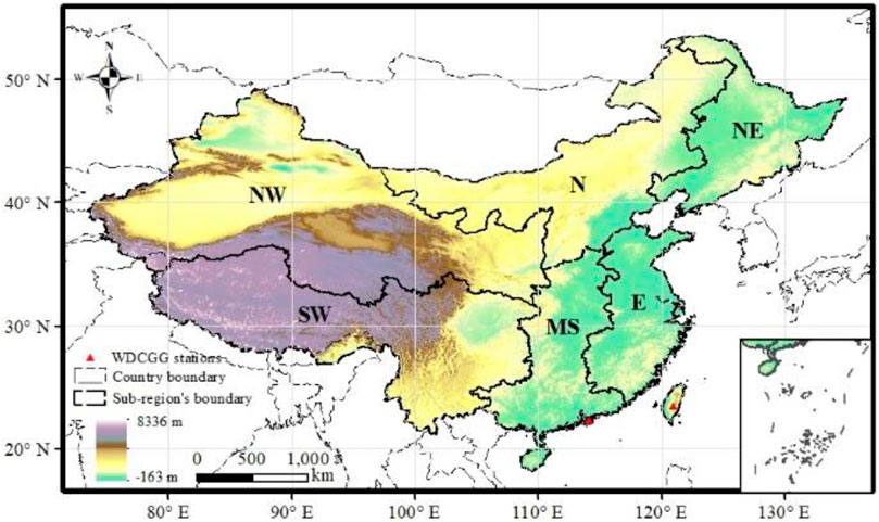
FIGURE 1. Geographic location and the six sub-regions of China. (NW is Northwest China, SW is Southwest China, N is North China, MS is Middle and South China, NE is Northeast China, and E is East China).
Four types of datasets are used in this study, namely, in situ observations, satellite remote sensing, model simulations, and reanalysis. As part of the validation process for gridded CO2 products, the in situ observation data from WDCGG were utilized, and the satellite and modeled CO2 products were used to study the spatiotemporal variation of CO2 at different altitude. A driving mechanism analysis was conducted using gridded data from the LAI and CDIAC, as well as ERA5 reanalysis data. Supplementary Table S1 provides a brief overview of all datasets used in this study.
The World Data Centre for Greenhouse Gases (WDCGG) has been operated by the Japan Meteorological Agency (JMA) since 1990 as part of the WMO/GAW program. As the only World Data Centre (WDC) specializing in greenhouse gases, it serves to collect, archive, and distribute greenhouse gas data from ground-, ship-, aircraft-, and satellite-based observations, contributed by organizations and individual researchers worldwide (WMO, 2012). The objective of the WDCGG is to support the monitoring of climate change and facilitate policy development, thereby helping reduce the risks associated with environmental degradation. In this study, the in situ observation data from the WDCGG were used to evaluate the performance of GOSAT and CT CO2 products in China.
GOSAT is the world’s first satellite dedicated to monitoring greenhouse gases from space, which was launched on 23 January 2009 and is jointly developed by the Ministry of Environment (MOE), the Japan Aerospace Exploration Agency (JAXA), and the Japan National Institute for Environmental Studies (NIES). GOSAT is a Sun-synchronous orbit at an altitude of 666 km, with an approximate 10.5 km diameter at nadir and a revisit cycle of 3 days (Yokota et al., 2009; Suto et al., 2021). A total of two observation instruments are onboard the satellite, the Thermal and Near-infrared Sensor for carbon Observation Fourier Transform Spectrometer (TANSO-FTS) and the TANSO-Cloud and Aerosol Imager (TANSO-CAI), which are designed to detect the three-dimensional distribution of greenhouse gases as well as clouds and aerosols. Both of them are equipped with four bands, and the three SWIR (0.76, 1.6, and 2.0 um) and the wide TIR (5.5–14.3 um) bands of TANSO-FTS are responsible for retrieving the column concentrations and vertical profiles of CO2 (Imasu et al., 2008). While the spectral channel of TANSO-CAI is used to capture the cloud cover and aerosol properties (Deng et al., 2016), the cloud-contaminated footprints are screened out according to this information. Based on these observations, the CO2 retrieval algorithms have been extensively developed, including NIES (Yoshida et al., 2013), ACOS (Kulawik et al., 2019), and UOL-FP (Oshchepkov et al., 2013), and the operational CO2 products are widely used in estimating the global and regional CO2 concentrations and fluxes.
In this study, we used the L4B global CO2 distribution dataset, which was developed by the Japan National Institute for Environmental Studies using the NIES-FP inversion algorithm. The latest version of this dataset is updated to V02.07 and can be freely accessed through www.gosat.nies.go.jp. It covers the period from June 2009 to October 2019, with a spatial resolution of 2.5 × 2.5 and a temporal resolution of 6 h over 17 vertical levels from the surface to 10 hPa. In order to obtain the atmospheric CO2 concentrations at different levels and time scales, the original netCDF format dataset was converted to raster images in the R programming environment, and then the daily, monthly, and annual average CO2 concentrations were aggregated from the hourly observations.
CarbonTracker (CT) is a data assimilation system for CO2 developed by NOAA ESRL. It incorporates a two-way nested offline atmospheric tracer transport model, known as transport model 5 (TM5), to simulate the surface fluxes and the distribution of atmospheric CO2 (Krol et al., 2005; Peters et al., 2007). CT separately estimates the surface CO2 exchange originating from fossil fuel emissions, terrestrial biosphere impacts, biomass burning, and ocean fluxes. In addition to in situ observations from tall towers, flask samples collected by NOAA’s cooperative air sampling network, and continuous measurements taken by partners, CarbonTracker assimilates more than 100 datasets around the world. By utilizing the technology of an ensemble Kalman filter, the differences between observations and model forecasts are reduced (Peters et al., 2005; Babenhauserheide et al., 2015). The model provides global 3D CO2 distribution at 25 levels with 3 × 2 (longitude × latitude) spatial resolution and 3 h temporal resolution. In this study, CarbonTracker data of version CT 2019B were collected for evaluating the impacts of anthropogenic, biogenic, wildfire, and oceanic sources on the concentrations of atmospheric CO2.
It is acknowledged that human activity and the biophysical process of vegetation play an indispensable role in affecting near-surface CO2 concentrations (Cao et al., 2019; Yang et al., 2021). Therefore, the leaf area index (LAI) and fossil fuel carbon emissions were employed to investigate the relationship between local CO2 and anthropogenic and biogenic factors. The LAI is defined as the one-sided green leaf area per ground surface and is a useful indicator in reflecting the canopy and functions of the vegetation community (Bréda, 2003). According to the study of Berterretche et al. (2005), the LAI shows a linear correlation with the primary production in terrestrial ecosystems, and the capacity of vegetation in carbon sequestration increases with the growing LAI. In this study, the LAI data were obtained from the Climate Data Record (CDR) developed by the National Centers for Environmental Information, which produced a daily LAI dataset on a 0.05 × 0.05-grid based on data derived from Advanced Very High Resolution Radiometer (AVHRR) sensors from 1981 onward. In order to minimize cloud contamination and atmospheric variability, this study employed a maximum value composite (MVC) procedure to generate monthly LAI.
The Carbon Dioxide Information Analysis Center (CDIAC), operated by the United States Department of Energy, is designed to provide global warming data and analysis to the U.S. government and research community (Andres et al., 2014). The primary mission of the CDIAC is committed to obtaining, evaluating, and distributing data related to greenhouse gas emissions and climate change. On the basis of monthly energy consumption data, the CDIAC divides the global total emissions into different sectors, such as fossil fuel emissions, industrial processes, and land use emissions (Oda et al., 2018). The monthly fossil fuel CO2 emissions of V2016, with a spatial resolution of 1 × 1 for 2009–2013, were selected in the present study.
ERA5 is the latest fifth-generation reanalysis dataset developed by the European Centre for Medium-Range Weather Forecasts (ECMWF) (https://www.ecmwf.int) and contains a series of improvements relative to its predecessor, ERA-Interim. The dataset employs an advanced data assimilation and modeling system with additional historical in situ and satellite observations to provide a more accurate representation of atmospheric conditions (Karl and Michela. 2019; Jiang et al., 2021). The spatial resolution of the data is 0.25°×0.25° on 37 vertical levels from the surface up to 1 hPa. It covers the period from 1959 to the present and is updated daily with a latency of 5 days. In this study, the monthly wind data of the reanalysis from 2009 to 2019 were used to derive the mean states of zonal and vertical movement of the atmosphere.
Due to the possibility that different datasets may differ in terms of their spatial and temporal references, all datasets were projected to the GCS_WGS_1984 geographic coordinate system and converted to local time of Beijing to maintain consistency. Additionally, to make the datasets comparable and facilitate the following analysis, the products of CT, LAI, and CDIAC were aggregated or resampled to a 2.5 × 2.5 regular grid by using the spatial information of GOSAT as a standard.
Prior to applying the estimated CO2 in the following analysis, the accuracy of GOSAT and CT in China was evaluated through comparison with WDCGG observations. Stations used for validation were screened based on the following criteria: (1) falling within the study area, (2) not being assimilated in generating the products of GOSAT and CT, and (3) having less than 20% of missing observations. For a gauge station, we first identified the grid cell in which that station was located in the spatial dataset of a satellite product. Then, the values of grid data were directly extracted and the Pearson linear correlation coefficient (R) and the root mean square error (RMSE) were used to measure the strength of the linear association and the magnitude of the deviation between observations and estimates. The formula is as follows:
where Pe and Po are the estimated and observed CO2, respectively; n is the sample size; δ is the standard deviation; and cov() is the covariance between the two variables.
In addition, the Pearson correlation method was also used to study the impacts of anthropogenic and biogenic activities on surface CO2 concentrations by calculating the correlation coefficients between LAI, fossil fuel carbon emissions, and local CO2 concentrations.
The interannual variation of CO2 was evaluated using linear trend fit as expressed in Eq. 3. The slope and statistical significance of the trends were estimated using the ordinary least squares method and the two-tailed Student’s t-test, respectively. In this study, a trend was considered statistically significant when it is at the 95% confidence level. In addition, the coefficient of variation (CV) was used to quantify the seasonal variation of CO2, and it was defined as the ratio of the standard deviation to the mean in Eq. 4.
where y is the time series of CO2 concentrations; a and b are the corresponding trend and the intercept, respectively; t represents the year; and ε is the regression error. s and‾x are the standard deviation and the mean of CO2, respectively.
As the concentration of CO2 exhibits a strong seasonal variation, it is thus essential to calculate the seasonal indexes and remove the seasonal factor from the time series when studying the multi-year monthly average CO2 concentrations and conducting the correlation analysis with fossil fuel carbon emissions and LAI (Dettinger and Ghil, 1998). In this study, the ts and decompose functions in R were used to deseasonalize the interannual variation of CO2, and the original time series were divided into three components: the trend component, the seasonal component, and the random component. After that, the seasonal component was subtracted from the time series and was treated as an input to the subsequent analysis.
where tsactual is the actual value of the dataset and tstrend, tsseason, and tsrandom are the trend component, seasonal component, and random component, respectively, of the time series.
After conducting the screening process, only the stations of LLN and HKO were considered to meet the criteria in China. The scatterplots between the observations and estimates are presented in Figures 2A, B. Generally, the CO2 estimates from GOSAT and CT agreed well with observations, with averaged correlation coefficients of 0.96 and 0.85 for LLN and HKO stations, respectively. The HKO station exhibited a slightly higher RMSE (6.88 ppm) than that in the LLN station (4.44 ppm). Both of the products had a CO2 estimation accuracy lower than 2%, meeting the requirements for precision described in Rayner and O'Brien (2001). In addition, the general pattern of intra-annual variations in CO2 can be well-captured by GOSAT and CT, which peaks in winter and reaches its lowest level in summer (Figures 2C, D). In light of the high accuracy and good stability of GOSAT and CT, the estimated CO2 products can be used to study the spatiotemporal patterns of CO2 in China.
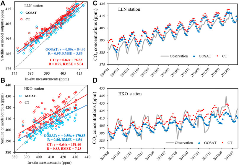
FIGURE 2. Scatterplots (A, B) and the comparison of time series (C, D) between in situ measurements and GOSAT and CT.
In order to study the spatiotemporal variations of CO2 concentrations at different heights of the atmosphere, three typical layers, namely, the 975 hPa, 500 hPa, and 100 hPa, were selected to represent the mean state of CO2 at the near surface, the middle, and the upper troposphere. The annual, seasonal, and diurnal variations of CO2 concentrations were analyzed at these three levels if there is no further specification.
The spatial pattern and magnitude of CO2 concentrations varied among different heights of the atmosphere. A declining trend was observed with increasing atmospheric height, with a mean CO2 concentration of 400.25 ppm at near surface decreasing to 398.41 ppm and 393.76 ppm at the middle and upper troposphere, respectively (Supplementary Table S2). Among them, the near surface witnessed a strong spatial heterogeneity with the highest concentrations of CO2 occurring in East China and the lowest in Northwest China (Figure 3A). This pattern is consistent with the spatial distribution of China’s population and economy, indicating a considerable impact of local carbon emissions on near-surface CO2. In contrast, CO2 concentrations at the middle troposphere showed much less variation, with a standard deviation of only 0.23 (Figure 3C). The insignificant variations may be associated with horizontal and vertical winds, which transport near-surface CO2 to the atmosphere and then sufficiently mixed, resulting in a uniform spatial pattern of CO2 concentrations (Cao et al., 2019; Al-Bayati et al., 2020). In the upper levels of the atmosphere, a distinct gradient of CO2 concentrations was observed from south to north (Figure 3E). High values of CO2 are concentrated in the area of low latitudes, while low CO2 values are observed at high latitudes. Such a phenomenon may be the result of large-scale circulation in the upper troposphere (Sohn et al., 2019).
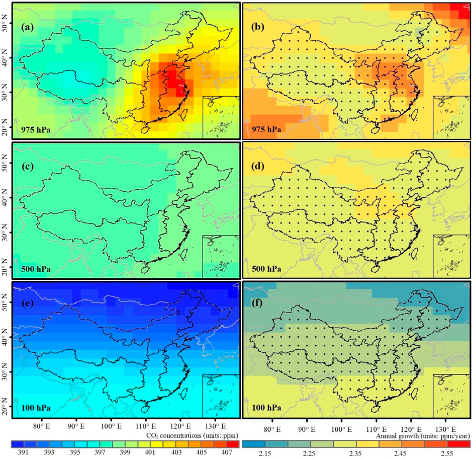
FIGURE 3. Spatial patterns of the annual mean (A, C, and E) and the change rates (B, D, and F) of CO2. It is to be noted that the grid cells filled with black dots indicate that the change rates are significant at the 95% level.
A general increasing trend with a magnitude higher than 2.1 ppm/year was detected for all the three typical layers (Figure 4), and almost all the data points passed the significance test at the 0.05 level (Figures 3B, D, F). Similar to the variation of CO2 concentrations, the annual change rate was significant at the near surface (2.38 ppm/year), where the high values of annual CO2 growth were found in part of East and North China. The middle troposphere witnessed a stable increasing trend at about 2.34 ppm/year. When it comes to the upper troposphere, the annual increase of CO2 shows large discrepancies across China, with high values in the Mid–South and low values in Northeast China. Based on the decreasing change rates from the lower to upper troposphere, it appears that the intensified anthropogenic activities tend to cause significant increase in CO2 at near surface.
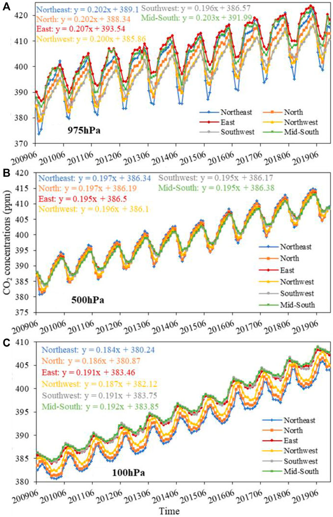
FIGURE 4. Interannual changes of CO2 concentrations during the period 2009–2019.
In order to study the intra-annual variation of CO2, the linear regression method was used to remove the annual growth rate, and then the monthly CO2 concentrations were derived by calculating the multi-year averages. At near surface, all the six regions exhibited a unimodal fluctuation pattern, with the peak value of CO2 concentrations occurring in April, followed by a decline, and reaching its trough in August (Figure 5A). This may be the result of the combined effect of anthropogenic and biogenic activities (WMO, 2017; Buchwitz et al., 2018). The increased photosynthesis of vegetation in summer is responsible for a higher uptake of CO2 from the atmosphere (Yang et al., 2021), while the intensified anthropogenic heating emissions and plant respiration lead to a higher level of CO2 in early spring (Liu et al., 2012). The amplitude of the seasonal variation is found to be largest in Northeast and lowest in East, and the differences between the peak and the trough are 24.14 and 12.80 ppm, respectively. In Northeast China, there is a strong seasonal difference in anthropogenic heating emissions and vegetation activity, while the anthropogenic CO2 is almost constant throughout the year in East; combined with the reduced seasonal variation in vegetation, the amplitude of seasonal variation of CO2 at East is smaller than that in Northeast China (Fang et al., 2014). A similar trend of CO2 seasonal variation was observed in the middle troposphere, with a high value in April and a low value in August (Figure 5B). The discrepancies among the six regions, however, are generally reduced, indicating the strong dilution effect of CO2 by vertical wind. In contrast, the CO2 variations at the upper troposphere exhibited an opposite trend, with the maximum CO2 concentrations observed in summer and the minimum CO2 concentrations in winter (Figure 5C). Such anomalies indicate that the upper troposphere CO2 was less affected by anthropogenic and biogenic activities. In addition, it was also found that CO2 concentrations in North China were generally higher than those in South China throughout the entire year. This may relate to the large-scale atmospheric circulation in the upper troposphere (Dargaville et al., 2000; Wang et al., 2011; Cao et al., 2019).
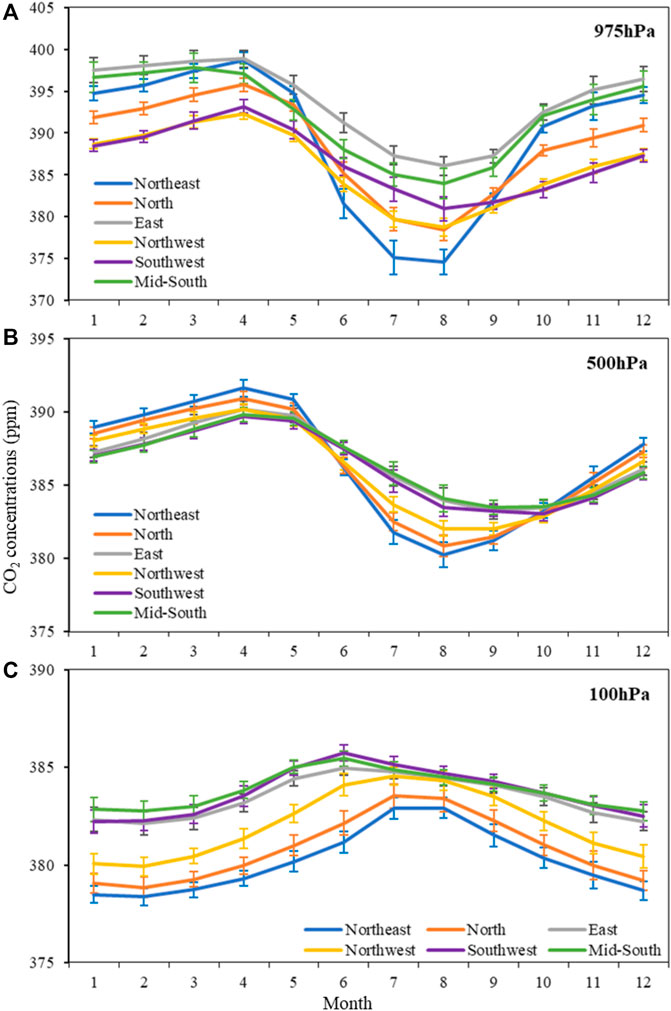
FIGURE 5. Monthly means of CO2 for the three typical layers over the period 2009–2019.
The seasonal variations of CO2 were found largest at the near surface, with a high value in spring and winter and a low value in summer and autumn (Figure 6). In particular, an apparent east–west difference in CO2 was observed across China, and the CO2 concentrations in the coastal provinces of Southeast China were generally higher than those in Northwest China throughout the year. At the middle troposphere, however, such spatial differences almost disappeared, while the temporal variations remained consistent with the lower troposphere. When it comes to the upper troposphere at 100 hPa, both the spatial and temporal variations of CO2 were the smallest among the three levels. The seasonal variation of the different levels was also reflected in the coefficient of variation, as shown in Supplementary Figure S1, with the largest CV of 1.45 found at 975 hPa and decreased to 0.79 and 0.36 at 500 hPa and 100 hPa, respectively. It is likely that the decreasing trend of CV is associated with the distance to the carbon sources and sinks at near surface. Therefore, we conclude that anthropogenic and vegetation activities are the main factors affecting the vertical distribution of CO2.
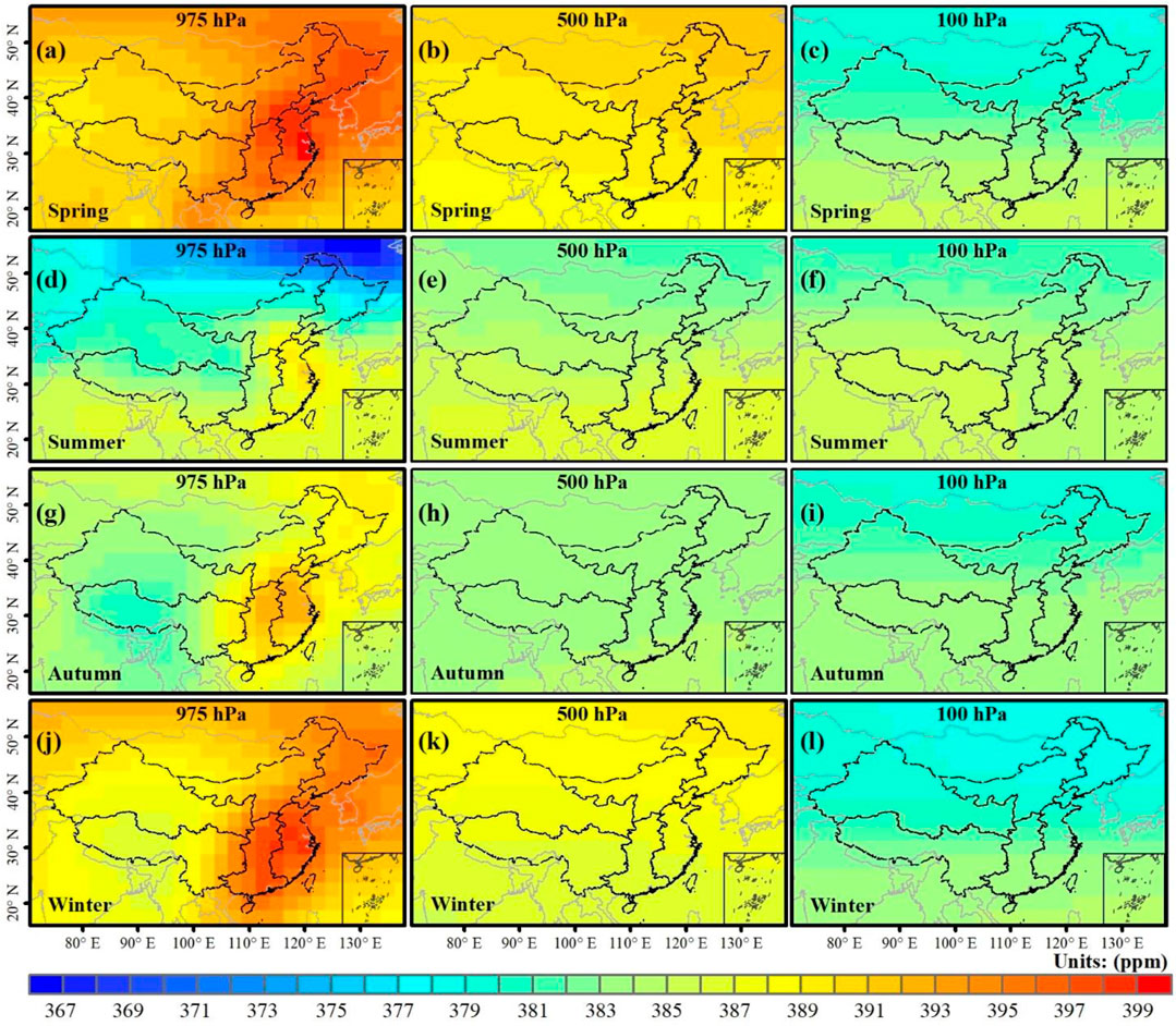
FIGURE 6. Spatial patterns of CO2 concentrations at four seasons for the three typical layers.
The mean diurnal amplitudes of CO2 variations at different levels and seasons are shown in Supplementary Table S3. In terms of vertical differences, the amplitude of the diurnal variation decreases from the near surface to the upper troposphere. The largest peak-to-trough diurnal amplitudes (8.90 ± 6.98 ppm) were found at the near surface, while the middle and the upper levels of the troposphere exhibited a smaller diurnal variability, with an amplitude of 0.88 ± 0.72 ppm and 0.44 ± 0.32 ppm, respectively. Such differences can be attributed to the transportation and dilution effects of the upper atmosphere, which make the diurnal cycles of CO2 at the middle and upper levels less affected by local sources and sinks.
As for the smallest amplitudes of diurnal variation of CO2 at the middle and upper troposphere, we are primarily interested in regional differences of daily CO2 variation at the near surface. Overall, a uniform diurnal cycle of CO2 was observed across the four seasons, with the trough occurring in the afternoon around 15:00, then turns to accumulate during nighttime and reaching its maximum at about 06:00 the next morning (Figure 7). It is possible that the obvious diurnal variations in CO2 throughout the whole year may be caused by active photosynthetic/respiratory fluxes in local vegetation (Li et al., 2004). As compared with spring and winter, summer and autumn witnessed relatively large amplitudes of CO2 variation. As for the regional differences in diurnal variations of CO2, Northwest and Southwest China exhibit an overall smaller amplitude than East China and other subregions, and there is almost no clear diurnal cycle during winter, which could be related to weak human and vegetation activities at high altitudes in western China (Shi et al., 2020; Lin et al., 2021).
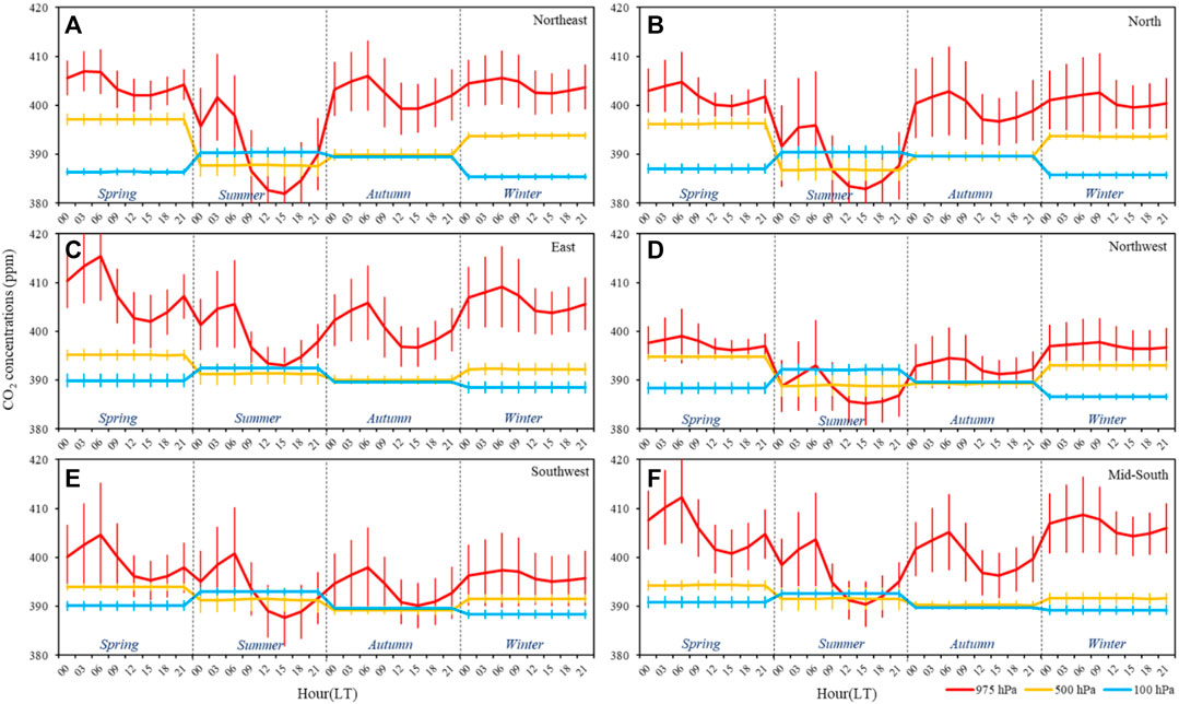
FIGURE 7. Diurnal cycles of CO2 for the six sub-regions across China.
Figure 8 illustrates the spatial distribution of the multi-year average atmospheric CO2 concentrations at different heights in China. CO2 concentrations at the near surface are generally higher than those at the top levels. CO2 concentrations exhibit a strong spatial heterogeneity at the height of 850 hPa and below, with high values observed in eastern China and lower values in western regions, probably caused by the local emissions of human activity. This east–west spatial difference gradually decreases with height and disappears at 150 hPa, a phenomenon that may be explained by the dilution and mixing effects of vertical wind. At the height of 100 hPa and above, there is a distinct south–north difference in the spatial distribution of CO2, with high CO2 concentrated at low latitudes and vice versa. This discrepancy may be attributed to the large-scale atmospheric circulation at the top troposphere.
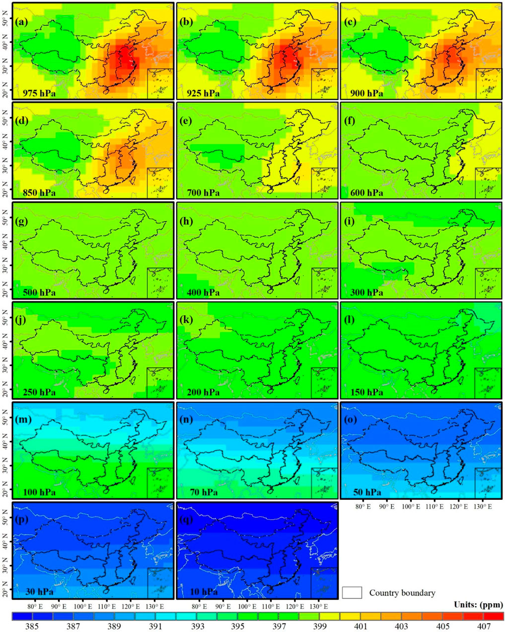
FIGURE 8. Spatial distribution of atmospheric CO2 over China at different height
In order to explore the regional differences of CO2 at different heights, the vertical profiles of CO2 for the six regions are shown in Figure 9A. The near surface (levels 1–5) witnessed the greatest discrepancy among the six regions, and then it decreased to 0 at the middle troposphere (levels 6–11). Smaller differences were observed at the upper troposphere (levels 12–17). The dilution effect of vertical wind allows local CO2 emissions to move upward with an increase in convective PBL, explaining the linear decrease in lower tropospheric CO2 in East and Mid–South China (Newman et al., 2013). When it comes to the middle troposphere, the mixing effect of zonal and vertical winds is the dominant factor, which makes the CO2 fully mixed and results in a small variation, whereas the continuous and regular atmospheric circulation contributes most to the smaller regional differences of CO2 at the upper troposphere (Dargaville et al., 2000; Sohn et al., 2019).
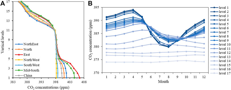
FIGURE 9. Vertical profiles (A) and the seasonal variation (B) of atmospheric CO2 over China.
To better understand the seasonal variation of CO2 at different heights, the linear regression method was used to remove the annual change rate from the calculation of the monthly mean CO2 concentration. As shown in Figure 9B, the seasonal fluctuations are gradually diminishing with increasing height. The peak-to-trough seasonal amplitude can be reached to 14.36 ppm at the height of 975 hPa, but it is reduced to less than 1 ppm above 50 hPa. In addition, a unimodal pattern of CO2 variation was observed below 500 hPa, with a peak value occurring in April and a trough in August. Nevertheless, at 400 hPa or higher, the peak and trough of CO2 occur 1 or 2 months later than at near surface. This further indicates that CO2 in the middle troposphere is transported by ground emissions.
According to the model results of CT, we evaluated the influence of anthropogenic, biogenic, oceanic, and fire sources in each of the six regions. It is to be noted that the biogenic and oceanic modules act as a carbon sink, a capability that has gradually strengthened over the past decade (Figures 10A, D). While the anthropogenic and fire activities exert a positive effect on local CO2 and shows an increasing trend as well (Figures 10B, C), in particular, the biogenic CO2 shows a similar pattern across the six regions, with maximum carbon sequestration occurring in September and the minimum occurring in May. The only difference is that there is another trough of carbon sequestration in January in the Northeast and the North, which is likely due to the inactive photosynthesis of vegetation in the cold season at high latitudes (Li et al., 2004). However, the regional differences in biogenic CO2 are much smaller than those of anthropogenic CO2. Carbon emissions from fossil fuels in the East and Mid-South are higher than those in the Northwest and Southwest throughout the year. The maximum difference of anthropogenic CO2 can reach 15 ppm in winter. Furthermore, a gentle flat variation of seasonal fossil fuel CO2 was also observed in western China. Contrary to the variation pattern of anthropogenic and biogenic CO2, the fire and oceanic CO2 exhibit the least regional differences with almost no seasonal variation, indicating that these two tracers of CO2 in China are transported by wildfire emissions and oceanic absorption in other places.
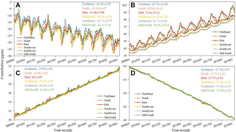
FIGURE 10. Simulated CO2 from biogenic (A), anthropogenic (B), fire (C), and oceanic (D) modules in CT at near surface
Because of the large differences of simulated anthropogenic and biogenic CO2 among the six regions, a completely independent dataset was used to verify the correlation between CO2 concentrations and the fossil fuel emissions and the vegetation activity and to explore the spatial differentiation of this relationship. According to the results of correlation analysis, the near-surface CO2 is significantly correlated with fossil fuel emissions on a national scale, with a correlation coefficient of 0.66 (Figure 11B). As for the grid scale, except for some sparsely populated areas such as desert, Gobi, and high mountains, where the correlation coefficient is negative, other areas show significant positive correlations (Figure 11A). Especially in parts of the Northwest and Southwest, the correlation coefficient is as high as 0.9, which indicates that fossil fuel emissions are the dominant factor affecting near-surface CO2 in less developed regions. However, this strong correlation appears to be declining in the East and Mid-South (R ≈ 0.7), which can be partly explained by the intensive land use change and the massive cement production (Gregg et al., 2008; Herzog, 2009).
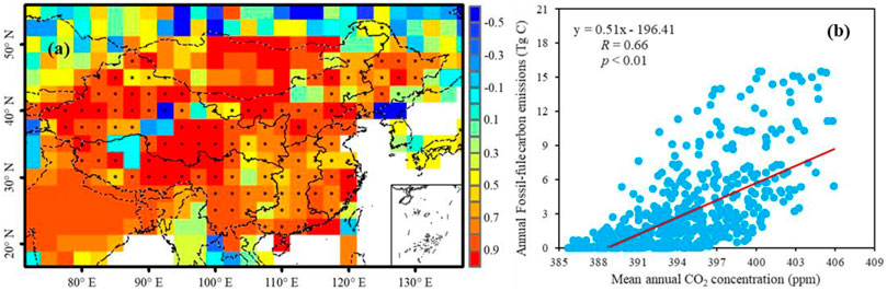
FIGURE 11. Correlation analysis between CO2 and fossil fuel carbon emissions on the grid (A) and national scale (B) at near surface. It is to be noted that the grid cells filled with black dots indicate that the correlation is significant at the 95% level.
Although a general positive correlation was observed between near-surface CO2 and fossil fuel emissions, however, there is no evidence to support that this is the cause of seasonal fluctuation in CO2. According to the study of Fung et al. (1997) and Van Der Velde et al., 2013, the flux of δ13C in the process of carbon exchange between the atmosphere and biosphere is evidently greater than that between the atmosphere and ocean. In order to study the influence of terrestrial ecosystems on seasonal variation of near surface CO2, the LAI was used to conduct a correlation analysis. As shown in Figures 12A, B, a completely opposite trend was observed between the near-surface CO2 and LAI, with a negative correlation coefficient being as high as −0.85. Photosynthesis of vegetation removes a relatively small amount of CO2 before March. From April onward, the LAI increases gradually and leads to a decrease in CO2, with the largest photosynthesis CO2 sequestration observed in August. Then, the monthly mean CO2 increases with a decrease in the LAI from autumn to early spring of the following year. In terms of spatial distribution, approximately 96% of the grid cells show a negative correlation, with strong correlation mainly distributed in eastern China and weak correlation in part of western provinces (Figure 12A). This east–west spatial difference may relate to the patterns of land use and land cover in China (Liu et al., 2008; Lin et al., 2021). The seasonal variation of CO2 is highly dependent on the LAI in areas where forestland, grassland, and cropland are concentrated, while showing a weak or even positive correlation in sparse vegetation and bare land.
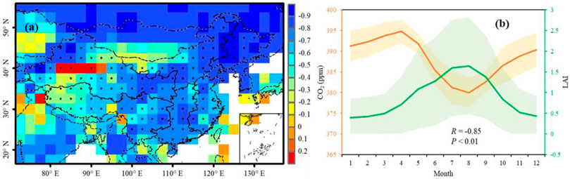
FIGURE 12. Correlation analysis between CO2 and LAI on the grid (A) and national scale (B) at near surface. It is to be noted that the grid cells filled with black dots indicate that the correlation is significant at the 95% level.
A similar approach was used to investigate whether fossil fuel carbon emissions and vegetation activity in China may have affected the CO2 concentrations at the middle and upper troposphere. As shown in Figure 13A, a completely opposite trend was observed between the middle tropospheric CO2 and LAI, with a negative correlation of −0.57. The variations of CO2 are lagged by 4 months on average relative to the LAI. Our results are consistent with those reported in the Northern Hemisphere, where the shortest lag phase was observed in the low latitudes and the longest in the region between 30°N and 40°N (Cao et al., 2019). When it comes to the upper levels of troposphere, the variation of CO2 exhibits a uniform pattern with the LAI (R = 0.92). It appears that vegetation carbon sequestration does not have an evident impact on upper tropospheric CO2. However, further research is required to determine why there is a strong correlation between CO2 at high altitudes and surface vegetation. The strong influence of fossil-fuel CO2 emissions on near-surface CO2 tends to weaken at higher levels of the troposphere, with a correlation coefficient decreasing to 0.47 and 0.23, respectively, for the middle and upper troposphere (Figures 13B, C). The reduced correlation indicates a dissipating effect of local carbon emissions on atmospheric CO2 with increasing altitude. As a result, we can conclude that the upper levels of atmospheric CO2 are less affected by local carbon sources and sinks; it is therefore important to take into account the influence of regional atmospheric circulation when conducting the driving force analysis (Sohn et al., 2019; Al-Bayati et al., 2020).
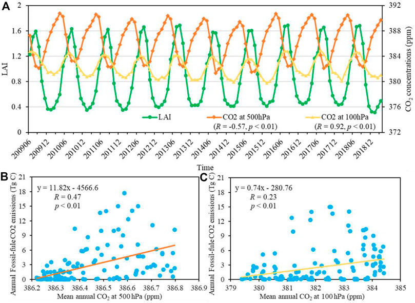
FIGURE 13. Interannual variability of LAI and CO2 (A) and the correlation analysis between CO2 and fossil fuel emissions (B, C) at the middle (500 hPa) and upper (100 hPa) levels of the troposphere.
Based on the wind data generated by ERA5, this study further explored the effects of atmospheric circulation in modulating the distribution of CO2 at the upper atmosphere. The wind field was decomposed into zonal and vertical winds, and then their influence on CO2 concentration at different heights was evaluated. At the height of 500 hPa, satellite observations indicate lower concentrations of CO2 in the northwest and southwest of China. These areas have low CO2 emission values and are dominated by the wind from the west and the southwest; the relatively low CO2 concentrations from upstream countries, such as India, Pakistan, and Central Asia, have less impact on western China (Figure 14B). In addition, the frequent air motion in the upward and downward directions facilitates the mixing of the upper and lower air (Figure 14A), which assists in CO2 dispersal. While the upward airflow was most prevalent in the Mid-south and eastern China, high CO2 concentrations from the ground were carried to the upper levels, in combination with the westerly wind, resulting in high CO2 concentrations in eastern China. Accordingly, the spatial distribution of CO2 at the middle of the troposphere is the result of a combination of near-surface carbon emissions and zonal and vertical air motions (Cao et al., 2019). At the height of 100 hPa, an obviously zonal circulation stratification is observed with a uniform westerly wind, whereas the vertical airflow is weak (Figures 14C, D). The distinct differentiation of CO2 from north to south reflects the zonal average distribution of atmospheric circulation at the global scale. Therefore, the spatial patterns of CO2 at the upper levels of the troposphere may largely be explained by zonal winds (Dargaville et al., 2000).
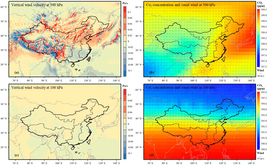
FIGURE 14. Multi-year average climatology of tropospheric circulation at the middle (500 hPa) and upper (100 hPa) troposphere, with (A, C) for the vertical wind velocity, and (B, D) for the zonal wind and the annual mean CO2 concentration.
Our results indicate an obvious increase in CO2 at the near surface and the middle troposphere at 2.38 ppm/year and 2.34 ppm/year, respectively, over the period from 2009 to 2019. The growth rate of CO2 at both levels is higher than the rate averaged for global areas (2.20 ppm/year and 2.34 ppm/year, respectively, for the near surface and middle troposphere) and Central Asia (Supplementary Table S4). As a result of the rapid development of China’s economy, such a trend is in accordance with the study of Peters et al. (2011), who reported a strong increment of atmospheric CO2 well above the global mean in the 21st century. It should be noted that the rate derived from satellite products is much lower than the rate obtained from in situ measurements at the regional scale (Fang et al., 2014; Cao et al., 2017). This difference may be the results of different sampling points used in the studies. As traditional in situ observation systems are not able to obtain the data in complex terrain regions, where the concentrations of CO2 are relatively low, using the values derived from satellite remote sensing may lower the regional averages. In addition, the different periods used may also have contributed to the differences. The growth rate of the study period including 2015, for example, is generally higher than that of the study period excluding 2015. Because the year 2015 is a typical El Niño–Southern Oscillation (ENSO) year, the growth rate of atmospheric CO2 is expected to increase due to the anomalous sea surface warming, and covering the analysis period in that year may have yielded a higher rate of annual growth of CO2 (Schwalm et al., 2011; Kim et al., 2016).
The improved accuracy of satellite CO2 products has created new opportunities for studying the spatiotemporal variations of CO2 in areas where field observations are inadequately sampled. In this study, the annual, seasonal, and diurnal variations of CO2 at different heights across six sub-regions of China were examined. The results show consistently increasing of CO2 with a magnitude higher than 2.1 ppm/year for all levels of the troposphere, and the seasonal cycles of CO2 at the near surface and the middle troposphere are similar, with a high value in the early spring and a low value in summer, which exhibit an opposite trend to the upper troposphere. An obvious spatial heterogeneity was observed at the near surface, with the highest concentration of CO2 occurring in East China and the lowest in Northwest China. This strong spatial heterogeneity, however, disappeared as the height increased and was replaced by a distinct south–north gradient difference at the upper troposphere. The diurnal variation of CO2 was found to be the largest in eastern China, whereas the western part exhibits a smaller variation. In terms of vertical variation, the concentrations of CO2 at the lower troposphere are generally higher than the values at the upper troposphere. Similar trends were also found in both the annual and seasonal variations of CO2. According to the driving mechanism analysis, the variation of CO2 at the near surface is mainly affected by the anthropogenic and biogenic activities, whereas the regional atmospheric circulation dominates the spatial distribution of CO2 at the upper troposphere.
Continuous monitoring of CO2 is the foundation for understanding the spatial distribution of carbon sources and sinks and for studying the regional carbon cycle (Dettinger and Ghil, 1998; Hammerling et al., 2012; Peters et al., 2012). This study presented a comprehensive analysis of the spatiotemporal patterns of atmospheric CO2. The results show a large discrepancy of CO2 concentrations and driving mechanisms among the six subregions of China. Thus, it is necessary to take the background concentration and the distinctive driving forces into consideration when formulating strategies for reducing carbon emissions (Zeng et al., 2013; Lin et al., 2021). Although the coarser temporal and spatial resolution of GOSAT may limit the representativeness of CO2 at fine scale, it contributes to understanding the spatiotemporal pattern and the variability of CO2 in China. With a more extensive CO2 observation network established and the continuous improvements in the technology of numerical simulation, future studies should integrate multi-source datasets from in situ and remote sensing measurements and model forecast to conduct a further in-depth assessment of atmospheric CO2 in China.
Publicly available datasets were analyzed in this study. These data can be found at: https://www.gosat.nies.go.jp and https://gml.noaa.gov/ccgg/carbontracker/.
Conceptualization, XJ and XD; methodology, XD; software, RD and QX; validation, JC; formal analysis, XJ; investigation, YH and YW; resources, SZ; data curation, SZ; writing—original draft preparation, XJ; writing—review and editing, XJ and XD; visualization, XJ; supervision, CJ and XD; project administration, MC; funding acquisition, YH and MC All authors have read and agreed to the published version of the manuscript.
This work was supported by the Joint Fund of Anhui Natural Science Foundation (2208085UQ03), the Innovation Development Program of China Meteorological Administration (No. CXFZ2022J046), the Anhui research project in the public interest (1604f0804003), and the Special innovation and development project of Anhui Meteorological Bureau (CXB202202).
The authors declare that the research was conducted in the absence of any commercial or financial relationships that could be construed as a potential conflict of interest.
All claims expressed in this article are solely those of the authors and do not necessarily represent those of their affiliated organizations, or those of the publisher, the editors, and the reviewers. Any product that may be evaluated in this article, or claim that may be made by its manufacturer, is not guaranteed or endorsed by the publisher.
The Supplementary Material for this article can be found online at: https://www.frontiersin.org/articles/10.3389/fenvs.2023.1129639/full#supplementary-material
Al-Bayati, R. M., Adeeb, H. Q., Al-Salihi, A. M., and Al-Timimi, Y. K. (2020). The relationship between the concentration of carbon dioxide and wind using GIS. United States: AIP Publishing LLC, 050042.
Andres, R. J., Boden, T. A., and Higdon, D. (2014). A new evaluation of the uncertainty associated with CDIAC estimates of fossil fuel carbon dioxide emission. Tellus B: Chem. Phys. Meteorology 66 (1), 23616. doi:10.3402/tellusb.v66.23616
Babenhauserheide, A., Basu, S., Houweling, S., Peters, W., and Butz, A. (2015). Comparing the CarbonTracker and TM5-4DVar data assimilation systems for CO2 surface flux inversions. Atmos. Chem. Phys. 15 (17), 9747–9763. doi:10.5194/acp-15-9747-2015
Basu, S., Guerlet, S., Butz, A., Houweling, S., Hasekamp, O., Aben, I., et al. (2013). Global CO2 fluxes estimated from GOSAT retrievals of total column CO2. Atmos. Chem. Phys. 13 (17), 8695–8717. doi:10.5194/acp-13-8695-2013
Berterretche, M., Hudak, A. T., Cohen, W. B., Maiersperger, T. K., Gower, S. T., and Dungan, J. (2005). Comparison of regression and geostatistical methods for mapping Leaf Area Index (LAI) with Landsat ETM+ data over a boreal forest. Remote Sens. Environ. 96 (1), 49–61. doi:10.1016/j.rse.2005.01.014
Bréda, N. J. (2003). Ground-based measurements of leaf area index: A review of methods, instruments and current controversies. J. Exp. Bot. 54 (392), 2403–2417. doi:10.1093/jxb/erg263
Buchwitz, M., Reuter, M., Schneising, O., Noël, S., Gier, B., Bovensmann, H., et al. (2018). Computation and analysis of atmospheric carbon dioxide annual mean growth rates from satellite observations during 2003–2016. Atmos. Chem. Phys. 18 (23), 17355–17370. doi:10.5194/acp-18-17355-2018
Cao, L., Chen, X., Zhang, C., Kurban, A., Qian, J., Pan, T., et al. (2019). The global spatiotemporal distribution of the mid-tropospheric CO2 concentration and analysis of the controlling factors. Remote Sens. 11 (1), 94. doi:10.3390/rs11010094
Cao, L., Chen, X., Zhang, C., Kurban, A., Yuan, X., Pan, T., et al. (2017). The temporal and spatial distributions of the near-surface CO2 concentrations in Central Asia and analysis of their controlling factors. Atmosphere 8 (5), 85. doi:10.3390/atmos8050085
Crisp, D. (2015). Measuring atmospheric carbon dioxide from space with the Orbiting Carbon Observatory-2 (OCO-2). Earth Obs. Syst. xx 9607, 960702. doi:10.1117/12.2187291
Dargaville, R., Law, R., and Pribac, F. (2000). Implications of interannual variability in atmospheric circulation on modeled CO2 concentrations and source estimates. Glob. Biogeochem. Cycles 14 (3), 931–943. doi:10.1029/1999gb001166
Deng, F., Jones, D. B., O'dell, C. W., Nassar, R., and Parazoo, N. C. (2016). Combining GOSAT XCO2 observations over land and ocean to improve regional CO2 flux estimates. J. Geophys. Res. Atmos. 121 (4), 1896–1913. doi:10.1002/2015jd024157
Dettinger, M. D., and Ghil, M. (1998). Seasonal and interannual variations of atmospheric CO2 and climate. Tellus B 50 (1), 1–24. doi:10.1034/j.1600-0889.1998.00001.x
Du, J., Wang, K., Wang, J., and Ma, Q. (2017). Contributions of surface solar radiation and precipitation to the spatiotemporal patterns of surface and air warming in China from 1960 to 2003. Atmos. Chem. Phys. 17 (8), 4931–4944. doi:10.5194/acp-17-4931-2017
Fang, S., Zhou, L., Tans, P., Ciais, P., Steinbacher, M., Xu, L., et al. (2014). In situ measurement of atmospheric CO<sub>2</sub> at the four WMO/GAW stations in China. Atmos. Chem. Phys. 14 (5), 2541–2554. doi:10.5194/acp-14-2541-2014
Fung, I., Field, C., Berry, J., Thompson, M., Randerson, J., Malmström, C., et al. (1997). Carbon 13 exchanges between the atmosphere and biosphere. Glob. Biogeochem. Cycles 11 (4), 507–533. doi:10.1029/97gb01751
Gregg, J. S., Andres, R. J., and Marland, G. (2008). China: Emissions pattern of the world leader in CO2 emissions from fossil fuel consumption and cement production. Geophys. Res. Lett. 35 (8), L08806. doi:10.1029/2007gl032887
Hammerling, D. M., Michalak, A. M., and Kawa, S. R. (2012). Mapping of CO2 at high spatiotemporal resolution using satellite observations: Global distributions from OCO-2. J. Geophys. Res. Atmos. 117 (D6). doi:10.1029/2011jd017015
Herzog, T. (2009). World greenhouse gas emissions in 2005. D.C., United States: World Resources Institute.
Imasu, R., Saitoh, N., Niwa, Y., Suto, H., Kuze, A., Shiomi, K., et al. (2008). Radiometric calibration accuracy of GOSAT-TANSO-FTS (TIR) relating to CO2 retrieval error. Noumea, New Caledonia: SPIE, 102–109.
Jiang, Q., Li, W., Fan, Z., He, X., Sun, W., Chen, S., et al. (2021). Evaluation of the ERA5 reanalysis precipitation dataset over Chinese Mainland. J. hydrology 595, 125660. doi:10.1016/j.jhydrol.2020.125660
Karl, H., and Michela, G. (2019). What is ERA5. Available at: https://confluence.ecmwf.int/display/CKB/What+is+ERA5 (Accessed 12 11, 2022).
Kim, J. S., Kug, J. S., Yoon, J. H., and Jeong, S. J. (2016). Increased atmospheric CO2 growth rate during El Niño driven by reduced terrestrial productivity in the CMIP5 ESMs. J. Clim. 29 (24), 8783–8805. doi:10.1175/jcli-d-14-00672.1
Kong, Y., Chen, B., and Measho, S. (2019). Spatio-temporal consistency evaluation of XCO2 retrievals from GOSAT and OCO-2 based on TCCON and model data for joint utilization in carbon cycle research. Atmosphere 10 (7), 354. doi:10.3390/atmos10070354
Kramer, R. J., He, H., Soden, B. J., Oreopoulos, L., Myhre, G., Forster, P. M., et al. (2021). Observational evidence of increasing global radiative forcing. Geophys. Res. Lett. 48 (7), e2020GL091585. doi:10.1029/2020gl091585
Krol, M., Houweling, S., Bregman, B., Van Den Broek, M., Segers, A., Van Velthoven, P., et al. (2005). The two-way nested global chemistry-transport zoom model TM5: Algorithm and applications. Atmos. Chem. Phys. 5 (2), 417–432. doi:10.5194/acp-5-417-2005
Kulawik, S. S., Crowell, S., Baker, D., Liu, J., Mckain, K., Sweeney, C., et al. (2019). Characterization of OCO-2 and ACOS-GOSAT biases and errors for CO 2 flux estimates. Atmos. Meas. Tech. Discuss. 2019, 1–61.
Le Quéré, C., Andres, R. J., Boden, T., Conway, T., Houghton, R. A., House, J. I., et al. (2012). The global carbon budget 1959–2011. Earth Syst. Sci. Data Discuss. 5 (2), 165–185. doi:10.5194/essd-5-165-2013
Li, K., Wang, S., and Cao, M. (2004). Vegetation and soil carbon storage in China. Sci. China Ser. d earth sciences-english edition- 47 (1), 49–57. doi:10.1360/02yd0029
Lin, Q., Zhang, L., Qiu, B., Zhao, Y., and Wei, C. (2021). Spatiotemporal analysis of land use patterns on carbon emissions in China. Land 10 (2), 141. doi:10.3390/land10020141
Liu, H., Feng, J., Järvi, L., and Vesala, T. (2012). Four-year (2006–2009) eddy covariance measurements of CO2 flux over an urban area in Beijing. Atmos. Chem. Phys. 12 (17), 7881–7892. doi:10.5194/acp-12-7881-2012
Liu, H., Zhao, P., Lu, P., Wang, Y-S., Lin, Y-B., and Rao, X-Q. (2008). Greenhouse gas fluxes from soils of different land-use types in a hilly area of South China. Agric. Ecosyst. Environ. 124 (1-2), 125–135. doi:10.1016/j.agee.2007.09.002
Liu, Y., Wang, J., Yao, L., Chen, X., Cai, Z., Yang, D., et al. (2018). The TanSat mission: Preliminary global observations. Sci. Bull. 63 (18), 1200–1207. doi:10.1016/j.scib.2018.08.004
Mustafa, F., Bu, L., Wang, Q., Ali, M. A., Bilal, M., Shahzaman, M., et al. (2020). Multi-year comparison of CO2 concentration from NOAA carbon tracker reanalysis model with data from GOSAT and OCO-2 over Asia. Remote Sens. 12 (15), 2498. doi:10.3390/rs12152498
Newman, S., Jeong, S., Fischer, M., Xu, X., Haman, C., Lefer, B., et al. (2013). Diurnal tracking of anthropogenic CO2 emissions in the Los Angeles basin megacity during spring 2010. Atmos. Chem. Phys. 13 (8), 4359–4372. doi:10.5194/acp-13-4359-2013
Oda, T., Maksyutov, S., and Andres, R. J. (2018). The open-source data inventory for anthropogenic CO2 version 2016 (ODIAC2016): A global monthly fossil fuel CO2 gridded emissions data product for tracer transport simulations and surface flux inversions. Earth Syst. Sci. Data 10 (1), 87–107. doi:10.5194/essd-10-87-2018
Oshchepkov, S., Bril, A., Yokota, T., Wennberg, P. O., Deutscher, N. M., Wunch, D., et al. (2013). Effects of atmospheric light scattering on spectroscopic observations of greenhouse gases from space. Part 2: Algorithm intercomparison in the GOSAT data processing for CO2 retrievals over TCCON sites. J. Geophys. Res. Atmos. 118 (3), 1493–1512. doi:10.1002/jgrd.50146
Peters, G. P., Marland, G., Le Quéré, C., Boden, T., Canadell, J. G., and Raupach, M. R. (2012). Rapid growth in CO2 emissions after the 2008–2009 global financial crisis. Nat. Clim. change 2 (1), 2–4. doi:10.1038/nclimate1332
Peters, G. P., Minx, J. C., Weber, C. L., and Edenhofer, O. (2011). Growth in emission transfers via international trade from 1990 to 2008. Proc. Natl. Acad. Sci. 108 (21), 8903–8908. doi:10.1073/pnas.1006388108
Peters, W., Jacobson, A. R., Sweeney, C., Andrews, A. E., Conway, T. J., Masarie, K., et al. (2007). An atmospheric perspective on North American carbon dioxide exchange: CarbonTracker. Proc. Natl. Acad. Sci. 104 (48), 18925–18930. doi:10.1073/pnas.0708986104
Peters, W., Miller, J., Whitaker, J., Denning, A., Hirsch, A., Krol, M., et al. (2005). An ensemble data assimilation system to estimate CO2 surface fluxes from atmospheric trace gas observations. J. Geophys. Res. Atmos. 110 (D24), D24304. doi:10.1029/2005jd006157
Rayner, P. J., and O'Brien, D. M. (2001). The utility of remotely sensed CO2 concentration data in surface source inversions. Geophys. Res. Lett. 28 (1), 175–178. doi:10.1029/2000gl011912
Schneising, O. (2008). Analysis and interpretation of satellite measurements in the near-infrared spectral region: Atmospheric carbon dioxide and methane. Bremen, Germany: Universität Bremen.
Schwalm, C. R., Williams, C. A., Schaefer, K., Baker, I., Collatz, G. J., and Rödenbeck, C. (2011). Does terrestrial drought explain global CO 2 flux anomalies induced by El Niño? Biogeosciences 8 (9), 2493–2506. doi:10.5194/bg-8-2493-2011
Shi, Y., Xi, Z., Simayi, M., Li, J., and Xie, S. (2020). Scattered coal is the largest source of ambient volatile organic compounds during the heating season in Beijing. Atmos. Chem. Phys. 20 (15), 9351–9369. doi:10.5194/acp-20-9351-2020
Sohn, B-J., Yeh, S-W., Lee, A., and Lau, W. K. (2019). Regulation of atmospheric circulation controlling the tropical Pacific precipitation change in response to CO2 increases. Nat. Commun. 10 (1), 1108–8. doi:10.1038/s41467-019-08913-8
Stocker, T., Qin, D., Plattner, G., Tignor, M., Allen, S., Boschung, J., et al. (2013). Contribution of working group I to the fifth assessment report of the intergovernmental panel on climate change. Clim. change 5, 1–1552.
Suto, H., Kataoka, F., Kikuchi, N., Knuteson, R. O., Butz, A., Haun, M., et al. (2021). Thermal and near-infrared sensor for carbon observation Fourier transform spectrometer-2 (TANSO-FTS-2) on the Greenhouse gases Observing SATellite-2 (GOSAT-2) during its first year in orbit. Atmos. Meas. Tech. 14 (3), 2013–2039. doi:10.5194/amt-14-2013-2021
Umezawa, T., Matsueda, H., Sawa, Y., Niwa, Y., Machida, T., and Zhou, L. (2018). Seasonal evaluation of tropospheric CO2 over the Asia-Pacific region observed by the CONTRAIL commercial airliner measurements. Atmos. Chem. Phys. 18 (20), 14851–14866. doi:10.5194/acp-18-14851-2018
Van Der Velde, I., Miller, J., Schaefer, K., Masarie, K., Denning, S., White, J., et al. (2013). Biosphere model simulations of interannual variability in terrestrial 13C/12C exchange. Glob. Biogeochem. Cycles 27 (3), 637–649. doi:10.1002/gbc.20048
Wang, J., Jiang, X., Chahine, M. T., Liang, M. C., Olsen, E. T., Yung, Y. L., et al. (2011). The influence of tropospheric biennial oscillation on mid-tropospheric CO2. Geophys. Res. Lett. 38 (20). doi:10.1029/2011gl049288
Wmo, G. (2017). The state of greenhouse gases in the atmosphere based on global observations through 2016. WMO Greenh. Gas. Bull. 13.
WMO (2012). World data Centre for greenhouse gases (WDCGG) data summary: Greenhouse gases and other atmospheric gases. Japan: Japan Meteorological Agency.
Yang, Y., Zhou, M., Wang, T., Yao, B., Han, P., Ji, D., et al. (2021). Spatial and temporal variations of CO2 mole fractions observed at Beijing, Xianghe, and Xinglong in North China. Atmos. Chem. Phys. 21 (15), 11741–11757. doi:10.5194/acp-21-11741-2021
Yokota, T., Yoshida, Y., Eguchi, N., Ota, Y., Tanaka, T., Watanabe, H., et al. (2009). Global concentrations of CO2 and CH4 retrieved from GOSAT: First preliminary results. Sola 5, 160–163. doi:10.2151/sola.2009-041
Yoshida, Y., Kikuchi, N., Morino, I., Uchino, O., Oshchepkov, S., Bril, A., et al. (2013). Improvement of the retrieval algorithm for GOSAT SWIR XCO2 and XCH4 and their validation using TCCON data. Atmos. Meas. Tech. 6 (6), 1533–1547. doi:10.5194/amt-6-1533-2013
Keywords: carbon dioxide, GOSAT, spatiotemporal variation, driving forces, China
Citation: Jin X, Deng X, Chen J, Zhu S, Huo Y, Dai R, Xu Q, Cao M and Wu Y (2023) A comprehensive evaluation of the spatiotemporal variation of CO2 and its driving forces over China. Front. Environ. Sci. 11:1129639. doi: 10.3389/fenvs.2023.1129639
Received: 22 December 2022; Accepted: 02 March 2023;
Published: 17 March 2023.
Edited by:
Haipeng Yu, Northwest Institute of Eco-Environment and Resources (CAS), ChinaReviewed by:
Yuanjian Yang, Nanjing University of Information Science and Technology, ChinaCopyright © 2023 Jin, Deng, Chen, Zhu, Huo, Dai, Xu, Cao and Wu. This is an open-access article distributed under the terms of the Creative Commons Attribution License (CC BY). The use, distribution or reproduction in other forums is permitted, provided the original author(s) and the copyright owner(s) are credited and that the original publication in this journal is cited, in accordance with accepted academic practice. No use, distribution or reproduction is permitted which does not comply with these terms.
*Correspondence: Xueliang Deng, ZGVuZ3h1ZWxpYW5nOTk4OUBhbGl5dW4uY29t
Disclaimer: All claims expressed in this article are solely those of the authors and do not necessarily represent those of their affiliated organizations, or those of the publisher, the editors and the reviewers. Any product that may be evaluated in this article or claim that may be made by its manufacturer is not guaranteed or endorsed by the publisher.
Research integrity at Frontiers
Learn more about the work of our research integrity team to safeguard the quality of each article we publish.