Spectrum sensing-focused cognitive radio network for 5G revolution

The cognitive radio network (CRN), an instrumental part of the next-generation wireless communication systems, is mainly dependent on spectrum sensing to function properly. The radio spectrum can help in clean energy transition and load capacity factors by providing a more efficient and accurate spectrum utilization. By using it, the number of spectrums that is used for communication can be optimized, which can reduce the amount of energy consumed by the network. Additionally, 5G radio spectrum sensing can be used to identify and classify different types of signals, which can help reduce the amount of interference in the network and improve the efficiency of energy utilization. It can also allow for the digitization of clean energy infrastructure and facilitate better decision-making processes that take into account environmental impacts while optimizing energy use because of its efficient characteristics like non-linearity, detection, scalability, robustness, generalization, non-stationarity in wireless environments, dynamic entity, weighted sum of Gaussian functions centered at specific frequencies, and robustness against noise and interference. It can adapt to noise and interference by adjusting its parameters, and this allows accurate distinguishing between primary and secondary users in the wireless spectrum, which is why a radial basis function is a popular choice for spectrum sensing in 5G networks. Radial basis function networks (RBFNs) can work better in 5G spectrum sensing for better signal classification, dynamic adaptation, fast detection, faster decision-making, and improved noise and interference reduction. One of the most sought-after goals in the field of wireless research is the creation of spectrum-sensing technology that is dependable and intelligent because multilayer learning approaches are inappropriate for dealing with time-series data due to the higher misclassification rate and inherent computational complexity. To address this, the study proposed the radial basis function network that learns the temporal aspects from spectral data and makes use of additional environmental statistics such as frequency, efficiency, energy, spectrum allocation, distance, and duty-cycle time, which are considered environmental data that may be used to fine-tune sensor performance. The scheme is simulated with real-time parameters, and the results are quite promising in terms of evaluation parameters.

1 Introduction

Spectrum development and network system compatibility are significant issues in realizing the complete vision and benefits for future generations (Ali & He, 2019; Ali et al., 2020). Furthermore, such policies may foster the development and competitiveness of innovative spectrum techniques and services that may be useful in energy management and environmental safety. A licensed spectrum can temporarily be accessed by secondary users (SUs) using a cognitive radio network, when there is no principal user. In backward induction, each SU performs the task of sensing the spectrum and conveying the details to the central controller. AI has become essential for effective communication in recent years. 5G standards are compatible with wireless equipment. Cognitive radio (CR) is a type of sophisticated scientific communication, in which the radio spectrum uses are managed (Devaraj et al., 2022). Interference during spectrum sensing, detection, and transmission requires the use of orthogonal frequency division multiplexing (OFDM) based on the cognitive radio network co-operative spectrum awareness resource allocation (CRN-CSS) (Meena & Rajendran, 2022). Ultra-dense networks (UDNs) provide high-throughput high-performance and user-centric wireless access to 5G deployments. Cognitive Radio integrates UDNs with legacy systems without allocating new airwaves, which would be expensive. The research reflects the advantages and disadvantages of the most widely known algorithm of this type, energy detection (ED), its probability, and performance evaluation (Ivanov et al., 2022). Co-operative communication in 5G networks is a rapidly evolving field that will be vital for the efficiency of future spectrums. Cognitive radio systems must recognize primary/principal (licensed) users across a large spectrum with a specified location and time. The consideration of user participation is motivated by the notion that sharing power and computing with adjacent nodes results in network energy resource savings (Banumathi et al., 2022). Wireless applications encounter spectrum overcrowding. Network obstruction causing call dropouts is another worry. These issues must be resolved for 5G and beyond to overcome spectrum overpopulation and networking. Therefore, energy detection and efficiency prediction is being determined (Eappen et al., 2022). Spectrum inadequacy causes roll-out, planning, and execution challenges for 5G and beyond. The growing number of wireless customers, traffic needs, poor spectrum distribution, and co-existence issues causes this spectrum deficit. A free wireless spectrum is essential. Using cognitive radio’s spectrum-sensing functionality in-between the sub-THz band range (0.1–1 THz) for beyond the 5G communication networks, the open spectrum can be forecasted and modeled. Therefore, energy detection, prediction, accuracy, probability, and time detection are examined in this research (Kansal et al., 2022). Wireless technology reduces spectrum resources. The ability to detect and analyze signals over a broad frequency range is an essential part of cognitive radio systems. So, wideband spectrum sensing is a crucial, important, and essential part of cognitive radio technology, allowing for dynamic spectrum allocation and function properly. However, the energy detection and allocation resource technique is performed to utilize the energy resources (Ju et al., 2021). The remaining portions of this study are arranged as follows: Section 2 presents the literature review. The proposed methodology is described in Section 3. The findings and discussion in Section 4 are followed by the conclusion in Section 5.

2 Literature review

In wireless channels, it is necessary to have accurate path loss prediction models to achieve correct signal propagation and energy detection. The deterministic and empirical methods utilized to predict path loss did not produce the best possible outcomes. Support vector regression and radial basis function (RBF) models were evaluated to increase the precision of path loss predictions in the environment (Mohanakurup et al., 2022). The accomplishment of the visible light communication (VLC) system is severely hindered because of the non-linearity that is caused by light-emitting diodes (LEDs), which interferes with the regular transmission and reception processes. A post-distorter for orthogonal frequency-division multiplexing depends upon very low power communication, which solves the problem that is caused by the non-linearity of LEDs. To apply non-linearity mitigations, the radial basis function interpolation, which is well-known for being an outstanding approach for function approximation, is being examined (Ojo et al., 2022). Light-emitting diodes used in visible light communication systems are the principal causative factors behind signal distortion due to their intrinsic non-linear features. The polynomial method is used to construct the post-distorter to mitigate the non-linear effect that is caused by the LED to increase the reliability of the system. The non-linear effect can also be mitigated with the use of radial basis function interpolation, which possesses powerful processing capabilities and high levels of solution accuracy (Zhang et al., 2022). These systems use a wide range of optoelectronic components, including photodiodes. LEDs’ non-linear features impose constraints on the system’s performance. Meanwhile, the high peak-to-average power ratio generated with the orthogonal frequency-division multiplexing modulation worsens the non-linear distortion, which is why it is desirable to mitigate the impacts of a non-linear distortion. The authors purposed radial basis function interpolation and employed a post-distortion technique combining RBF with memory effect depression (MED), which effectively suppresses the non-linear and memory effects of LEDs. Their goal is to target the non-linear characteristics of LEDs, and to do so, we employ radial basis function interpolation (Chen et al., 2022). It is observed that the superconducting technology-based hardware implementation of signal microprocessors could be useful for a variety of specialized jobs, in which both performance and energy efficiency are of the utmost importance. Within the scope of this research, based on radial basis functions, we examine the essential components of superconducting neural networks (RBF) (Schegolev et al., 2022). Qureshi et al. (2014) presented a multiple relay selection scheme for underlay CRN in CSI. In this regard, they utilized FRBs and swarm intelligence to reduce the transmit power. The scheme seemed promising in terms of energy efficiency, but its time complexity was substantial. Therefore, we proposed a technique for intelligently reducing the transmit power in underlay CRN and multiple relay selection. The concept was inspired by the Artificial Bee Colony (ABC) (Rahman et al., 2014). The scheme was efficient in energy-saving but costly in terms of computational complexity. RBF neural networks are considered universal optimizing networks and have been applied in the telecommunication field and other areas, and are one of the successful options for deep learning systems. In this regard, some of the most well-known algorithms in the relevant body of research are extreme learning machines (ELMs) and long short-term-based systems.

  Algorithm RBF -Net (K, A, 0) Input:

  Sequence of labeled training patterns Z = ((X₁, Y₁)… (X_i, Y_i))

  Number of RBF centers K

  Regularization constant ⁁

  Number of iterations O

  Initialize:

Run K-means clustering to find initial values for µ_K and determine $\sigma$ _k, k = 1, K, as the distance between µ_K and the closest µ_i. (I ≠ k).

  Do for o= 1: O.

  Compute optimal output weights w = (G^T G + 2⁁/i)⁻¹ G^TY.

  Compute gradients $\frac{\partial }{\partial uk}E$ and $\frac{\partial }{\partial uk}E$ as in and with optimal w and form a gradient vector v

3 Proposed methodology

3.1 Algorithm overview

RBF networks are utilized in mathematical modeling. This network activates with the radial basis function. The network output is a linear combination of neuron parameters and input RBFs. RBF networks can approximate functions, predict time series, classify data, and control systems. Broomhead and Lowe, Royal Signals and Radar Establishment researchers, initially formulated them in 1988. Radial basis function networks follow the conventional organizational format of three layers (input layer, hidden layer with a non-linear RBF activation function, and output layer with a linear function), where the input layer serves as the basis for the network and the hidden layer serves as the actual activation function. An acceptable representation for the input is a vector of real values. This scalar nature of the network’s output may be seen in the following equation, which relates input and output vectors:

Estimate the conjugate direction Ā with the Fletcher–Reeves–Polak–Ribiere CG method.

Perform a line search to find the minimizing step size $\mathcal{s}$ direction Ā; in each evaluation of E recomputed the optimal output weights w as in line 1.

Update $\sigma k$ and $\mu k$ with Ā and $\mathcal{s}$

Output: Optimized RBF net.

3.2 Proposed model

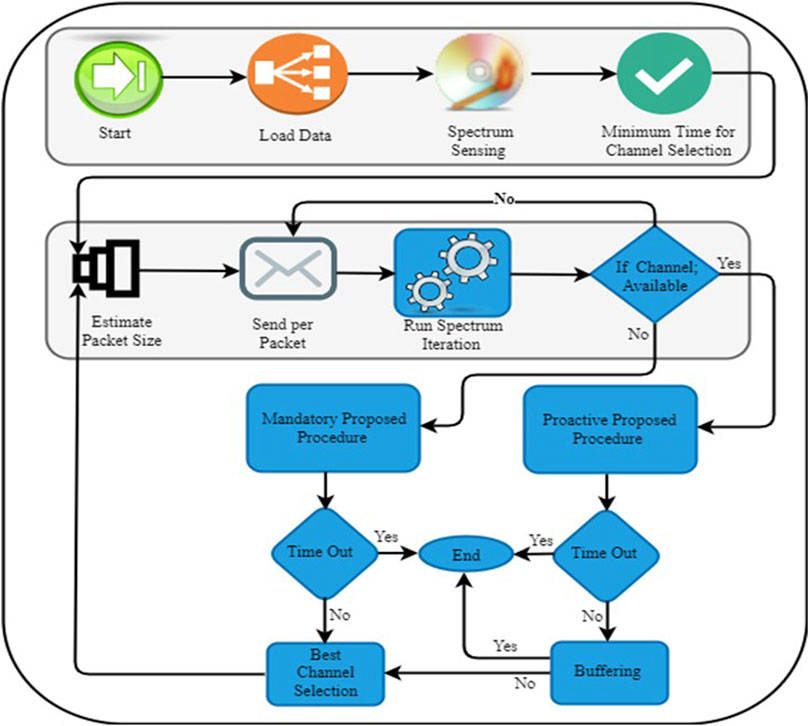
Figure 1 shows that the length of the packet shown the same as that of all other packets and then data are transmitted. Following that, spectrum sensing is performed again to examine the current channel’s operational state. If there is still space available on the channel, it will simultaneously transmit the second packet. This process can be repeated until all packet transmissions have been completed (provided that no arrival occurred during the transmission time). Even if the presently used channel is empty, the transmitter node will seek to switch to a different channel to free up the bandwidth that is being used by the present channel. This is referred to as PHO, which stands for "Proactive Hand Off.” If the user has already been using the current channel before the actual transmission, then a HO should be made in a reactive or required manner as follows: the algorithm that we discussed is displayed in this figure. For 5G communications, TDMA, OFDMA, and CDMA are used to guarantee that no customers’ signals would interfere with one another. This suggested work (CDMA) is enough to serve the requirements of the people who utilize wireless networks due to the rapid expansion of mobile devices. NOMA is gaining importance in 5G networks for multi-access systems. Multiple users can share the same frequency resources. There are two primary categories of domains: code and power; both are fundamental to NOMA approaches, and both will be covered in this article. In the previous section, we established that the power domain will serve as the principal focus of our investigation. In this configuration, many users can share the same time and frequency of resources to complete their respective data transfers. By superposing the signals of several users, all of them may share the same transmission channels. Subsequent interference cancellation, or SIC, is subsequently carried out to decipher the signals that users are meant to transmit and removes interference at the receiver end.

FIGURE 1

FIGURE 1. Proposed architecture for delay-sensitive image transmission in cognitive radio networks.

3.2.1 Dataset

This dataset includes over-the-air observations of legitimate radio signals modulated using eleven unique modulations generated from real-world radio broadcasts. This dataset was collected to compile this information. According to the authors, the signals were produced with the help of a USRP B210, which was linked to a computer operating GNU Radio to accomplish this goal. It was crucial to employ the same data sources and source code as before, when building the numerous transmitters, as they had to be compatible with RadioML 2016.10A. It is important to mention, to provide extra clarity, that earlier versions of the RadioML dataset contained discordantly with AM modulations. As a result of this discrepancy, the RadioML dataset was updated to correct future releases.

3.2.2 Network architecture

Radial basis function networks are typically multilayer networks consisting of an input layer, a hidden layer employing a non-linear RBF activation function, and a linear output layer. RBF network is the abbreviated form of radial basis function network. It would be feasible to depict the input modeled as a vector of real numbers, x∈ Rn. After that, the network’s output is a scalar function of the input vector, φ∶R^n →R; it is given as follows:

$\phi \left(x\right)={\displaystyle \sum _{i=1}^N}{a}_i\mathrm{P}\left(‖x-c_i‖\right).(1)$

To determine neuron I’s weight in the linear output neuron, we use the following formula: N = number of neurons in the hidden layer, Ci = neuron I’s center vector, and I = neuron I’s weight. Here, we figure out how many neurons reside in the deepest part of the network. The term “radial basis function” refers to the functions that are radially symmetrical about a given vector and whose behavior is determined solely by the distance from a certain center vector. In its most fundamental form, each hidden neuron receives input from all the other hidden neurons. The Euclidean distance is generally considered a standard, even though the Mahalanobis distance [28] seems to perform better in pattern identification, and the radial basis function is typically considered to be the norm Gaussian function:

$\mathrm{\rho }\left(‖x-c_i‖\right)=\exp \left[{{\beta }_i‖x-c_i‖}^2\right..(2)$

Since Gaussian basis functions are constrained to the central vector, changing the parameters of a single neuron has a minor impact on the input values placed at the neuron’s periphery:

$\underset{‖x‖\to \infty }{\lim }\rho \left(‖x-c_i‖\right)=0.(3)$

For a constrained region of Rn, RBF networks provide universal approximations under modest restrictions about the activation function’s form. This indicates that every continuous function on a closed, limited set may be approximated arbitrarily well by an RBF network with sufficiently hidden neurons.

3.2.3 Normalized architecture

Although RBF networks are often unnormalized, they may also be normalized in the way that was previously explained. An example of such a mapping is a normalized radial basis function:

$\left(\phi \right)X\stackrel{\scriptscriptstyle\mathrm{def}}{=}\frac{{\displaystyle \sum _{i-1}^N}\alpha i\rho \left(‖X-ci‖\right)}{{\displaystyle \sum _{i-1}^N}\rho \left(‖X-ci‖\right)}={\displaystyle \sum _{i-1}^N}\alpha iu\left(‖X-ci‖\right),(4)$

where

$u\left(‖X-ci‖\right)\stackrel{\scriptscriptstyle\mathrm{def}}{=}\frac{\rho \left(‖x-c_i‖\right)}{{\displaystyle \sum _{j-1}^N}\rho \left(‖X-ci‖\right)}.(5)$

3.2.4 Training RBF

Generally, RBF networks are trained using pairs of input and target values, X(t), Y(t), t-1…by a two-step algorithm

$K\left(W\right)\stackrel{\scriptscriptstyle\mathrm{def}}{=}{\displaystyle \sum _{t-1}^T}{K}_t\left(W\right),(6)$

where

$u\left(‖X-ci‖\right)\stackrel{\scriptscriptstyle\mathrm{def}}{=}\frac{\rho \left(‖x-c_i‖\right)}{{\displaystyle \sum _{j-1}^N}\rho \left(‖X-ci‖\right)}.(7)$

Selecting the Ci-centers of RBFs in the hidden layer is the initial step, which may be accomplished in various ways; for instance, the centers can be selected at random from a given set of samples, or they can be established through the utilization of K-means clustering. We have to take into account the fact that this phase does not have any supervision. In the second stage, a linear model with coefficient Wi is applied to the outputs of the hidden layer, while considering some objective function. A common example of an objective function is the least square function, which is used in regression analysis and function estimation:

$K_t\left(W\right)\stackrel{\scriptscriptstyle\mathrm{def}}{=}{\left[y\left(t\right)-\phi \left(X\left(t\right),W\right)\right]}^2.(8)$

Here, we explicitly included the dependency on the weights in the model. The precision of the fit can be improved by selecting the appropriate weights so that the objective function of least squares is minimized to its maximum. It is necessary to maximize not just one but several different goals, such as smoothness, in addition to accuracy. In such a scenario, maximizing a regularized objective function would be beneficial, such as the following:

$\mathrm{H}\left(\mathrm{W}\right)\stackrel{\scriptscriptstyle\mathrm{def}}{=}K\left(W\right)+\lambda S\left(W\right)=\mathit{def}{\displaystyle \sum _{t=1}^T}{H}_t\left(W\right),(9)$

where

$S\left(W\right)\stackrel{\scriptscriptstyle\mathrm{def}}{=}{\displaystyle \sum _{t=1}^T}{S}_t\left(W\right)(10)$

and

$H_t\left(W\right)\stackrel{\scriptscriptstyle\mathrm{def}}{=}{K}_t\left(W\right)+\lambda S_t\left(W\right).(11)$

4 Result and discussion

4.1 Discussion

4.1.1 Confusion metrics expression

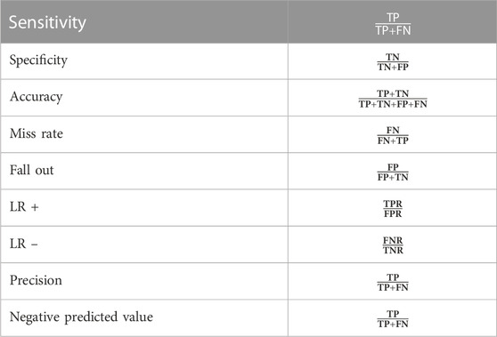
In the context of machine learning and, more specifically, the problem of statistical classification, confusion matrices, also known as error matrices, are used to evaluate the performance of an algorithm, often a supervised learning one. Confusion matrices are also known as error matrices (in unsupervised learning, it is usually called a matching matrix, please see Ref. Table 1). Either the first permutation, in which each row of the matrix represents the instances that correspond to an actual class, or the second, in which each column of the matrix represents the examples that belong to a predicted class, can be used for the inclusion of the error matrix. Named thus because it's easy to see whether the system is confusing two categories and incorrectly labeling one as the valid target.

TABLE 1

TABLE 1. Mathematical equations of confusion metrics.

Signal strength is an integer, whereas the other parameters are all expressed as floating-point numbers. Parameter 3 can assume values between 0 and 1, and the table has 1599 rows and 12 columns. Parameter 5 has a maximum allowable value of 0.6. The range of parameter 8 is quite narrow, from 0.9 to 1.004. Number 8 has the smallest standard deviation. Classifications for its 0.000187 “signal strength” are 3.5, 4.0, 5.0, 7.0, and 7.5. The mean, median, and mode are almost overlapping or too close to each other, except in parameter 7, and parameter 3 is trimodal and its signal strength is a classification variable. All of them are positively skewed. The standard deviation is the highest for parameter 7, i.e., 32.895324478299074. Class 5 has the highest count in “signal_strength.” Parameters 6 and 7 are highly correlated with each other and vice versa, and they have 0 correlations with another parameter. Parameter 1 is positively correlated with parameter 3 and parameter 8 and negatively correlated with parameter 2 and parameter 9. Parameter 4 has a very low correlation with other parameters. Parameter 4 has the highest number of outliners, which is 155, since the high coefficient value lies between ± 0.5 and ± 1. Parameter 1 is highly correlated with parameter 3 and parameter 8. Parameters 6 and 7 are highly correlated, but since the correlation is not too high near 0.8 and above, no decrease in feature support is observed. Almost all parameters have mean, median, and mode values that are too close together or overlap, except for parameter 7. Parameter 3 is trimodal, and signal strength is a categorical variable. They are all positively slanted in one direction or another. Parameter 7 has the largest standard deviation, with a value of −32.895324478299074. The highest count may be found in the “signal strength” of class 5. The correlation between parameters 6 and 7 is substantial, and they have no association with any other parameters. There is a positive correlation between parameters 1 and 3, and between parameters 1 and 8, but a negative correlation between parameters 1 and 9. The correlation between parameter 4 and the rest of the parameters is quite poor. The largest number of planners (total 155) may be found in parameter 4. As a result, the optimal range for coefficient values is 0.5–1. There is a strong relationship between parameter 1 and both parameter 3 and parameter 8. While there is a strong relationship between parameters 6 and 7, it is not strong enough to justify the elimination of feature support for them. The differences in variables are plotted in Figures 2A, B, C, respectively.

FIGURE 2

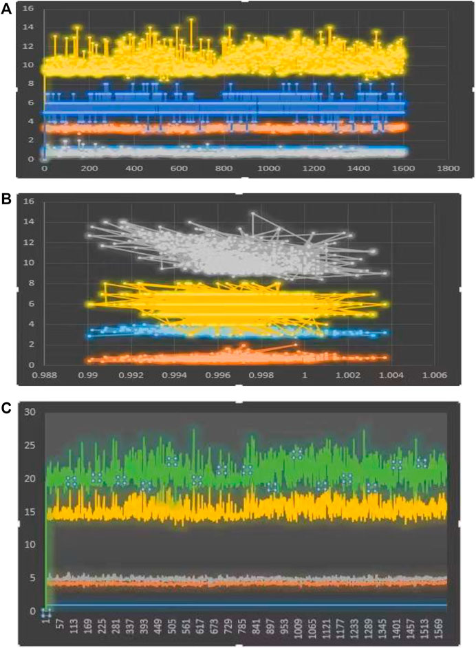
FIGURE 2. Differences in variations can be seen in Ref. (A-C) Signals variable parameters differences.

4.2 Results and analysis

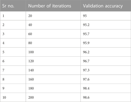
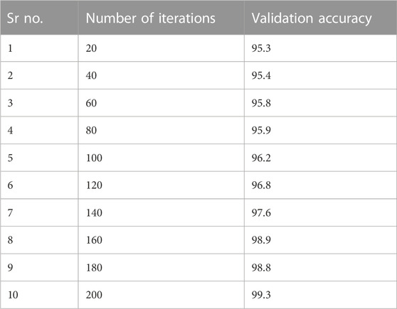
Seventy percent of the data is used for training the proposed model, while the remaining thirty percent is used for validation. The data are fed into the model in chunks, and the output functions are computed. Table 2, Table 3, and Table 4 provide the evaluation and validation results for the proposed model’s training and validation accuracies, respectively, while Figures 1, 3 provide graphical explanations of these results. The accuracy of both training and validation phases improves with an increase in iterations. Tables 3 and 4 show that the RBFN model selected has successfully dealt with the overfitting issue and is, therefore, well-suited for achieving the sought-after superior classification performance. When compared to six other algorithms, the RBFN’s 99.3 percent maximum performance is far higher than that of a normal energy detector, which achieves just 78 percent. Therefore, all algorithms may agree that the RBFN performance is satisfactory.

TABLE 2

TABLE 2. Validation accuracy for the proposed algorithms.

TABLE 3

TABLE 3. Training accuracy for the proposed algorithms.

TABLE 4

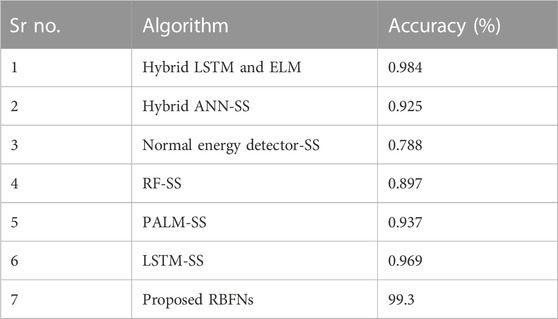
TABLE 4. Comparative study of algorithm performance from 45 to 2,207 MHz with a low signal-to-noise ratio (17 dBm–5 dBm) [9].

FIGURE 3

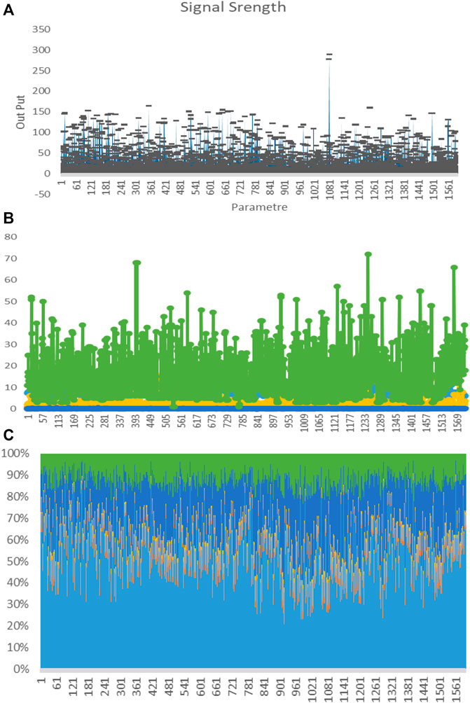
FIGURE 3. (A) Signal parameter and specific output. (B) Signal parameter and specific output. (C) Signal parameter and specific output.

4.3 Comparison of the proposed algorithm

Table 3 and Figure 5 analysis of existing algorithms with our proposed work at 45 to 2207 MHz and low to high SNR as −17 dBm to 5 dBm (decibel milliwatts). In Figures 4A, B, the training and validation of proposed algorithms show better accuracy than existing ones. Figure 3 shows the graphical representation of the analyzed algorithm with different bars.

FIGURE 4

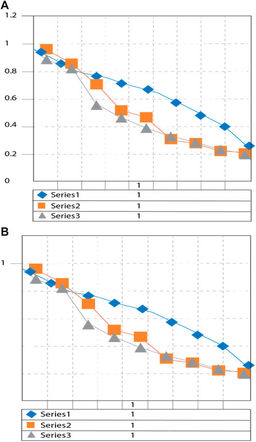
FIGURE 4. (A) Validation accuracy for the proposed algorithm. (B) Training accuracy for the proposed algorithm.

FIGURE 5

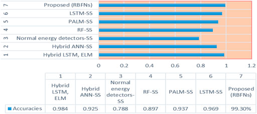
FIGURE 5. Analysis of the performance of the various methods at 45–2,207 MHz and low SNR (17 db–5 db).

5 Conclusion and future work

5G spectrum sensing can improve clean energy transition and load capacity factors by enhancing the environmental sustainability assessment through advanced statistical methods. It can allow for digitization of clean energy infrastructure and facilitate better decision-making processes that take into account the environmental impacts while optimizing energy use. Additionally, 5G spectrum sensing can help identify and analyze data related to the energy sources, their usage, and the associated environmental effects, which can provide insights that can be used to determine the best strategies for transitioning to clean energy sources and to increase the efficiency of energy networks and reduce the amount of energy used. Some of the reasons for choosing the RBFN are because it can be trained to classify different types of signals more accurately, such as differentiating between narrowband and wideband signals and detecting signal modulation schemes, noise reduction, and interference in the received signal, which can improve the accuracy of spectrum sensing. This can be carried out by training the network to recognize patterns in the received signal and filter out noise and interference. It can also be optimized to make faster decisions about the presence of primary users in the spectrum, which is important for real-time applications in 5G networks. Therefore, it can be designed to adapt to changes in the environment, such as variations in signal strength or the presence of other wireless devices by training the network on different scenarios and using adaptive learning algorithms. In this paper, we compared it to six other algorithms and found that RBFN's 99.3 percent maximum performance is far higher than that of a normal energy detector, which achieves just 78 percent. Therefore, all algorithms may agree that the RBFN performance provides satisfactory results, which are better than those of the previous studies in the literature. Additionally, the significant part of WSNs in spectrum sensing service transfer is studied, in which the RBFN performance was optimal. In addition, we also discussed the RBFN and its perspectives of frequency, efficiency, energy, and spectrum allocation. After doing a comprehensive analysis of the state of the art at the moment, we have identified several difficulties, some of which are quite remarkable, that call for more research.

Data availability statement

The original contributions presented in the study are included in the article/Supplementary Materials; further inquiries can be directed to the corresponding author.

Author contributions

All authors listed have made a substantial, direct, and intellectual contribution to the work and approved it for publication.

Funding

This work was supported by the National Natural Science Foundation of China under Grant nos. 51977153, 51977161, and 51577046, the State Key Program of the National Natural Science Foundation of China under Grant no. 51637004, the National Key Research and Development plan “important scientific instruments and equipment development” Grant no. 2016YFF0102200, and the Equipment Research Project in advance, Grant no. 41402040301.

Acknowledgments

The authors would like to thank the editors, the entire journal team, and the reviewers of their manuscript.

Conflict of interest

The authors declare that the research was conducted in the absence of any commercial or financial relationships that could be construed as a potential conflict of interest.

Publisher’s note

All claims expressed in this article are solely those of the authors and do not necessarily represent those of their affiliated organizations, or those of the publisher, the editors, and the reviewers. Any product that may be evaluated in this article, or claim that may be made by its manufacturer, is not guaranteed or endorsed by the publisher.

References

Ali, F. A., He, Y., Shi, G., Sui, Y., and Yuang, H. (2020). Future generation spectrum standardization for 5G and internet of Thin.gs. J. Commun. 15, 276–282. doi:10.12720/jcm.15.3.276-282

CrossRef Full Text | Google Scholar

Ali, F. A., and He, Y. (2019). “Spectrum for next generation technologies,” in Proceedings of the 2019 8th International Conference on Software and Information Engineering, Cairo, Egypt, April 2019.

CrossRef Full Text | Google Scholar

Banumathi, J., Sangeetha, S. K. B., and Dhaya, R. (2022). “Robust cooperative spectrum sensing techniques for a practical framework employing cognitive radios in 5G networks,” in Artificial intelligent techniques for wireless communication and networking (John Wiley and Sons, Ltd, New York, NY, USA), 121–138. doi:10.1002/9781119821809.ch9

CrossRef Full Text | Google Scholar

Chen, N., Wang, J., Zhang, S., and Shen, B.-Z. (2022). Nonlinear compensation for direct current-biased optical orthogonal frequency division multiplexing visible light communication system based on radial basis function interpolation. Opt. Eng. 61 (8), 86102. doi:10.1117/1.oe.61.8.086102

CrossRef Full Text | Google Scholar

Devaraj, S. A., Aruna, T., Muthukumaran, N., and Roobert, A. A. (2022). Adaptive cluster-based heuristic approach in cognitive radio networks for 5G applications. Trans. Emerg. Telecommun. Technol. 33 (1). doi:10.1002/ett.4383

CrossRef Full Text | Google Scholar

Eappen, G., T, S., and Nilavalan, R. (2022). Cooperative relay spectrum sensing for cognitive radio network: Mutated MWOA-SNN approach. Appl. Soft Comput. 114, 108072. doi:10.1016/j.asoc.2021.108072

CrossRef Full Text | Google Scholar

Ivanov, A., Stoynov, V., Mihaylova, D., and Poulkov, V. (2022). Applicability assessment of energy detection spectrum sensing in cognitive radio based ultra-dense networks. AIP Conf. Proc. 2570 (1), 20011. doi:10.1063/5.0099506

CrossRef Full Text | Google Scholar

Ju, H., Cho, E., and Kim, S.-H. (2021). “Energy-detection based false alarm reduction in polar-coded uplink control channel transmission in 5G-NR,” in Proceedings of the 2021 IEEE 93rd Vehicular Technology Conference (VTC2021-Spring), Helsinki, Finland, April 2021, 1–6. doi:10.1109/VTC2021-Spring51267.2021.9448973

CrossRef Full Text | Google Scholar

Kansal, P., Gangadharappa, M., and Kumar, A. (2022). Long boosted memory algorithm for intelligent spectrum sensing in 5G and beyond systems. J. Netw. Syst. Manage. 30 (3), 41. doi:10.1007/s10922-022-09652-w

CrossRef Full Text | Google Scholar

Meena, M., and Rajendran, V. (2022). Spectrum sensing and resource allocation for proficient transmission in cognitive radio with 5G. IETE J. Res. 68 (3), 1772–1788. doi:10.1080/03772063.2019.1672585

CrossRef Full Text | Google Scholar

Mohanakurup, V., Baghela, V. S., Kumar, S., Srivastava, P. K., Doohan, N. V., Soni, M., et al. (2022). 5G cognitive radio networks using reliable hybrid deep learning based on spectrum sensing. Wirel. Commun. Mob. Comput. 2022, 1–17. doi:10.1155/2022/1830497

CrossRef Full Text | Google Scholar

Ojo, S., Sari, A., and Ojo, T. P. (2022). Path loss modeling: A machine learning based approach using support vector regression and radial basis function models. Open J. Appl. Sci. 12 (06), 990–1010. doi:10.4236/ojapps.2022.126068

CrossRef Full Text | Google Scholar

Qureshi, I. M., Malik, A. N., and Naseem, M. T. (2014). Dynamic resource allocation in OFDM systems using DE and FRBS. J. Intelligent Fuzzy Syst. 26 (4), 2035–2046. doi:10.3233/ifs-130880

CrossRef Full Text | Google Scholar

Rahman, A., Qureshi, I., Malik, A., and Naseem, M. (2014). A real time adaptive resource allocation scheme for OFDM systems using GRBF-neural networks and fuzzy rule base system. Int. Arab J. Inf. Technol. (IAJIT) 11 (6).

Google Scholar

Schegolev, A., Klenov, N. v., Bakurskiy, S. v., Soloviev, I. I., Kupriyanov, M., Sidorenko, A., et al. (2022). Tunable superconducting neurons for networks based on radial basis functions. Beilstein J. Nanotechnol. 13, 444–454. doi:10.3762/bjnano.13.37

PubMed Abstract | CrossRef Full Text | Google Scholar

Zhang, D., Wang, J., Tian, H., Shen, B.-Z., and Zhou, Y. (2022). Gauss–Newton iteration method for radial basis function-based postdistortions in visible light communication systems. Opt. Eng. 61 (9), 95108. doi:10.1117/1.oe.61.9.095108

CrossRef Full Text | Google Scholar