Assessments of surface water quality through the use of multivariate statistical techniques: A case study for the watershed of the Yuqiao Reservoir, China

In light of the fact that water quality has been threatened by human activities, apportionments of potential pollution sources are essential for water pollution control. Multivariate methods were used to assess the water quality in the Yuqiao Reservoir and its surrounding rivers in northern China to identify potential pollution sources and quantify their apportionment. Fifteen variables at 10 sites were surveyed monthly in 2015–2016. The quality at this location was acceptable according to the water quality index (WQI), except for special parameters including chemical oxygen demand (COD), total nitrogen (TN), total phosphorus (TP), and chlorophyll (chlα). Cluster analysis (CA) grouped these datasets into three seasonal groups, July–September, December–March, and the remaining months. Principal component analysis/factor analysis (PCA/FA) identified seven factors that accounted for 79.7%–86.4% of the total variance, and the main sources included cities, rural districts, industries, weather, fertilizers, upstream areas, and vehicles. Absolute principal component scores and multiple linear regression (APCS–MLR) modeling results show that the hierarchical contribution of main pollution sources was ranked in the following order: upstream (26.6%) > urban district pollution source (21.5%) > vehicle emission pollution source (10.9%) in the flood season, upstream (22.3%) > rural district pollution (19.8%) > fertilizer erosion (15.8%) in the normal season, and upstream (26.4%) > urban district pollution (19.0%) > fertilizer erosion (18.8%) in the dry season. Sources from upstream and urban districts explained the most proportion. The matrix was also subjected to positive matrix factorization (PMF). A comparison of PMF and APCS–MLR results showed significant differences in the contribution of potential pollution sources. The APCS–MLR model performed better, as evidenced by a more robust R² test. Measures should be discussed and implemented in managing upstream areas, sewage treatment facilities, and fertilizer and industrial application.

1 Introduction

Industrialization and urbanization have impacted human life over the past few centuries; however, these processes have also caused great water environmental catastrophes during this time. Overexploitation coupled with surface water pollution has threatened the security of the potable water supply (Meng et al., 2018; Fu et al., 2020). Water pollution poses a significant threat to public health, and its causes can be traced to domestic wastewater, industrial, and agricultural wastewater (Qin et al., 2020). A prerequisite for the control of domestic water pollution is to identify the source of pollution.

Water management poses a great challenge in dealing with pollutant reduction, especially in northern China. Only 34% of the surface water at the Haihe River basin, where the Yuqiao Reservoir is located, met the requirements for drinking water in 2015 (Ministry of Water Resources of the People’s Republic of China, 2015). Therefore, it is helpful for managers to use simple and widely used techniques to study seasonal and spatial variations and the apportionment of pollution sources to assess water quality. The multivariate statistical methods, as an alternative technique, accomplish a complete assessment of water quality and environmental status of the study area by using the multivariate datasets (Ustaoglu and Tepe, 2019). The major statistical techniques, such as cluster analysis (CA), discriminant analysis (DA), principal component analysis (PCA), factor analysis (FA), and multivariate linear regression (MLR), have been applied to assess surface water quality in past decades, and there are recent papers demonstrating the multivariate statistics can provide source estimation of any contaminant in surface water and other ecological subjects (Vega et al., 1998; Singh et al., 2005; Zhou et al., 2007; Aydin et al., 2021; Cuce et al., 2022; Topaldemir et al., 2022). These helped to identify the pollution sources in the surface water. In addition, absolute principal component score (APCS)–MLR and positive matrix factorization (PMF) models, which have evaluated contributions of potential pollution sources, have been widely used in the apportionment of air pollution and riverine pollution sources (Wang et al., 2013; Gholizadeh Haji et al., 2016;Liu et al., 2019a; Chen et al., 2019; Zhang et al., 2020; Su et al., 2021), suggesting the reliability and feasibility of using receptor models in apportionment of water pollution sources.

The Yuqiao Reservoir is a part of the Haihe basin surface water system in northern China. The local climate is characterized by warm and rainy summers, while cold and dry winters cause the local rivers to freeze and have minimal flow in winter. The reservoir is surrounded by farmlands, villages, towns, and industrial zones, resulting in serious nitrate pollution and a massive generation of undesirable water bodies littered with fungus and waterweeds in their eutrophic states (Zhao et al., 2007). It is essential for water contamination control measures to identify the element and source of water pollution sources here, especially regarding the control of pollution from nitrate and other nutrients. Previous studies on the Yuqiao Reservoir mainly focused on the composition of nitrogen in the shallow ground water, the analysis of the water quality status in 1990–2004, diffuse pollution, the source and migration factor of non-point source phosphorus, and forecasting water quality conditions in the future using a BP neural network (Zhang et al., 2003; Wang et al., 2004; Zhao et al., 2007; Lu and Yin, 2008; Xu et al., 2015). To sum up, the apportionment of pollution sources in a specific set of pollutants or simply assessing the condition in a set of pollutants was conducted in previous studies in the gathering area. However, there is a lack of pollution source analysis concerning mixing the elements of nutrients, salinity, and heavy metals.

The objective of this study is to conduct comprehensive research on the temporal changes in water quality and sources of pollutants in the Yuqiao Reservoir by using multivariate statistical methods. Specifically, this is accomplished by analyzing datasets within which 15 water quality parameters are obtained from 10 sites during a two-year monitoring period (2015–2016) and then by applying a Brown water quality index (WQI), CA, PCA/FA, and APCS–MLR technologies. In this way, this study can achieve 1) the analysis of the spatio-temporal patterns and assessment of the water quality in the Yuqiao Reservoir and the surrounding rivers and 2) the apportionment of the identified pollution source contributions to each of the water quality variables. Insights from our study have potential not only to provide scientific guidance for pollution liability and the domestic development of control initiatives to weaken pollution growth in the Yuqiao Reservoir, but also to provide a reference for the analysis of pollution sources in other typical watersheds. By applying the findings in this study, governments could take more flexible and targeted measures, such as treating eutrophic sewage in villages and controlling vehicle emissions.

2 Methodology

2.1 Study area and datasets

The Yuqiao Reservoir was located in the north China (NC), covering from 40.01° to 40.08° N, and 117.43° to 117.65° E. The reservoir covers an area of 86.8 km² and controls a basin area of 2,060 km². It was built in 1960s and mainly for the purpose of flood control and water supply. The Yuqiao Reservoir plays a great role in ensuring the sustainable development of Tianjin’s national economy and people’s living water (Ministry of Finance of the People’s Republic of China, 2021; Enorth.com, 2022). The water in the reservoir mostly comes from the Sha and the Lin rivers. The Sha River feeds the reservoir from the east, while the Li River flows into the Sha River upstream of the reservoir. This reservoir restored the water in the Lin River. The Zhou River is downstream of the reservoir, and its flow is controlled by sluices, which lie across the river to the west of the reservoir. The annual mean temperature is between 14.0°C and 14.1°C, and 612.95 mm of precipitation fell annually in 2015–2016, according to Tianjin Bureau of Statistics (Wu and Peng, 2016). The local freshwater can freeze in December, January, and February, as the daily average air temperature dips below 0°C (National Meteorological Center of CMA 1981). The image of land-use data in 2013 was uploaded to the ArcMap 10.2 software. It shows that the reservoir is surrounded by large areas of farmland (53.43%), villages (12.16%), and woodland (14.91%). Industrial areas (0.71%) and towns (0.70%) were scattered in the west (Figure 1).

FIGURE 1

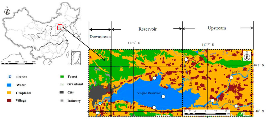
FIGURE 1. Land-use data image in the Yuqiao Reservoir.

Based on the hydrologic river features and previous results, 10 sampling sites around the Yuqiao Reservoir were selected. Four sites were upstream, three were at the reservoir, and the other two were downstream. Fifteen surface water quality parameters were chosen, including pH, water temperature (WT), dissolved oxygen (DO), chemical oxygen demand (COD), and electrical conductance (EC). Organic matters included total nitrogen (TN), total phosphorus (TP), ammonia nitrogen (NH₄⁺–N), nitrate, and nitrite. Also analyzed were three kinds of heavy-metal elements (Cu, As, and Hg), a biological parameter (chlorophyll, chlα), and the salt-based ion chloride (Cl⁻). In all, there were 308 data numbers. A HQ400 portable machine was used to attain the present pH, DO, and WT of the water. The measurement of nitrogen matter was conducted by the AutoAnalyzer 3, the measurement of chlα was conducted by the fluorescence of Trilogy, Turner Designs, and that of phosphorus was obtained with the help of molybdenum–antimony–scandium spectrophotometry. A titration method using silver nitrate was used to confirm the value of Cl⁻, and the content of heavy-metal elements used the spectrometer of ICP-AES (Yuksel and Arica, 2018), with a recovery percentage of 94.6%–101.2% for the certified reference material (CRM) of three heavy-metal elements in the text, and the LOD values of Cu, As, and Hg were 0.165, 0.025, and 0.005 μg/L, respectively. Analyses were carried out following the instructions in the Technical Specifications Requirements for Monitoring of Surface Water and Waste Water (Qi, 2002).

2.2 Water quality index

It is essential to understand the influences affecting the spatio-temporal variability in water quality to determine the quality of surface water and develop improvement strategies (Ustaoglu et al., 2021). A comprehensive value was needed as the process of the water quality assessment in the Yuqiao Reservoir was conducted. The Brown water quality index is a technique for evaluating water quality by grade and a common way to obtain the combined effect of each water quality parameter (Brown et al., 1972). Other criteria, based on the WQI, have been used to evaluate water quality in the United States and Canada. The parameters were ranked according to their weight value (AW), with values 1 and 5 (Supplementary Table S1), which were determined by their effect on water quality and importance for human health (Chai et al., 2021; Ustaoglu et al., 2020). Then, the relative weight (RW) was calculated by the ratio of AW to the sum of all AWs (Eq. 1). The quality rating (Q_i) was calculated by dividing the measured parameters (C_i) by the drinking water values, as permitted by the national surface water quality standard (State Environmental Protection Administration, 2002) type III, or the standard for drinking water sanitation (World Health Organization, 2011, Supplementary Table S2). The calculation of DO by Q_i is governed by Eq. 3, or Eq. 2 was used.

$RW=\frac{AW}{\sum AW},(1)$

$Q_i=\left(\frac{C_i}{S_i}\right)\times 100,(2)$

$Q_i=\left(\frac{S_i}{C_i}\right)\times 100,(3)$

where S_i represents the standard value of a specific parameter and C_i represents its observed value. S_i in Cl⁻ and nitrite follow the rules of WHO 2011 (World Health Organization, 2011), and the other parameters follow the rules of the China water quality standard (State Environmental Protection Administration, 2002). The sub-indices (SI_i) for this parameter were calculated by multiplying the RW and Q_i (Eq. 4). Finally, the WQIs are calculated by adding the sub-indices from different parameters (Eq. 5). The threshold water quality condition is given by WQI ≤ 100, which was a requirement for the water to meet the standards.

${SI}_i=RW\times Q_i,(4)$

$\mathrm{W}\mathrm{Q}\mathrm{I}={\displaystyle \sum }{SI}_i.(5)$

2.3 Cluster analysis

Because the original datasets were compiled monthly, it was necessary to cluster them to form seasons. Cluster analysis, as an unsupervised pattern recognition technique, is a common way to divide data into separate parts. CA classifies objects (cases) into classes (clusters/groups). Each object is analogous to the others in the cluster but different from those in other classes. The most similar observations are first grouped, and these initial groups are amalgamated based on their similarities (Kamble and Vijay. 2011). Eventually, as the similarity decreases, all subgroups are merged into a single cluster (Abbas et al., 2008). Hierarchical clustering analysis (HCA) is the most common approach to classify and analyze watershed water quality. It starts with the most similar pair of objects and forms higher clusters in a step-by-step fashion (Wang et al., 2013). The similarity of two samples is usually described by the Euclidean distance between two points (x) and (y) in p-dimensional space, which is given by:

$d\left(xy\right)={\left[{\displaystyle \sum }_{j=1}^p{\left(x_j-y_j\right)}^2\right]}^{1/2},(6)$

where d(xy) represents the Euclidean distance and j defines each parameter (Rafighdoust et al., 2016). HCA was performed on the normalized dataset using Ward’s method (Qin et al., 2020). Ward’s method uses an analysis of variance approach to evaluate the distances between clusters, attempting to minimize the sum of squares between any two clusters that can be formed at each step. In this research, we use hierarchical agglomerative CA to divide datasets into three parts: the dry season (DS), the normal season (NS), and the flood season (FS). The data were first grouped into months. The linear correlations between WT and DO (−0.579), EC (−0.523) were significant, and seasonal changes in WT, DO, and EC were notable. There were only three parameters (WT, DO, and EC) that were used in the HCA process, which generated a dendrogram (Supplementary Figure S1), essentially grouping 12 months into three clusters with significant differences. The seasonally changing parameters were used when clustering, including WT, DO, and EC, which proved to be more reasonable in their temporal pattern of water quality in this watershed and deemed suitable for other studies of water quality classification (Wang et al., 2013; Qin et al., 2020). According to the results of CA, the average levels of WT were 27.45°C, 17.48°C, and 4.54°C in the FS, the NS, and the DS, respectively. Meanwhile, the average DO for the FS, NS, and DS was 8.78, 9.56, and 13.08 mg/L, respectively. The average values of EC in the FS, NS, and DS were 0.57, 0.63, and 0.74 m/cm, respectively (Figure 2).

FIGURE 2

FIGURE 2. The Box plots of DO, EC, WT, and WQI in different seasons (the acceptable condition is DO ≥ 5 mg/L).

2.4 Principal component analysis and factor analysis

Principal component analysis (PCA) is a statistical method that uses the idea of dimensionality reduction. Under the premise of minimizing loss, multiple indexes are transformed into several comprehensive indexes composed of a linear combination of original variables, and these indexes are termed components.

Factor analysis (FA) is a method that captures common factors from variable groups and represents the original parameters using a linear combination of potential hypothetical and random influence variables. This process requires factor rotation and the rotated common factors are defined as varifactors (VFs). Different extraction results of VFs are caused by different rotation methods of extracted factors. The FA can be mathematically expressed as:

$z_{ij}=a_{f1}{f}_{1i}+a_{f2}{f}_{2i}+a_{f3}{f}_{3i}+\dots +a_{fm}{f}_{mi}+e_{fi},(7)$

where “z” is the measured variable, “a” is the factor loading, “f” is the factor score, “e” is the residual term accounting for errors or other source of variation, “i” is the sample number, and “m” is the total number of factors (Fraga et al., 2020).

The difference between PCA/FA and the origin PCA comes from rotating the axis defined by PCA (Shrestha et al., 2008; Soltani et al., 2020). The main purpose of FA is to reduce the contribution of less significant variables to simplify even more of the data structure coming from PCA (Fraga et al., 2020). This study used the varimax rotation method to analyze the PCA/FA. With the help of PCA/FA, the pollution sources in different seasons, represented by VFs, were extracted.

2.5 Source apportionment using the APCS–MLR receptor model

APCS–MLR is a numerical method used for allocating the contributions of each water pollution sources after isolating them using PCA/FA. It combines the multiple linear regression model and absolute principal component scores. The x variables of this model are the absolute factor scores, and the y variables are the concentrations of pollutants. This approach converts the APCS analysis factor score for the contribution of each pollution source according to the regression index provided by the APCS–MLR. Regression coefficients were obtained to estimate the contribution rate of each principal component to water quality variables. A detailed description of the receptor model was given by Thurston and Spengler (1985). The source contributions to the whole pollutant’s concentration (C_j) can be expressed as follows:

$C_{j={\left(r_0\right)}_j}+{\displaystyle \sum }_{k=1}^n{r}_{jk}\times {APCS}_k,(8)$

where (r₀)_j is a constant term of multiple regressions for pollutant j; r_jk is the coefficient of multiple regression of source k to j; APCS_k is the scaled value of the rotated k for the considered sample; and r_jk×APCS_k represents the contribution of source k to C_j, noting that the mean of the term r_jk × APCS_k on all monitored samples is the average contribution of the sources and that the ratio of the mean value of the r_jk×APCS_k to C_j represents the contribution to pollutant j. This multivariate receptor model, constructed with SPSS software, used the absolute factor scores as independent variables, while the chemical concentrations as the dependent variables (Li et al., 2011).

As the negative influence of factors on water quality variables exists, negative contributions are obtained for some pollution sources and, in some cases, it leads to contributions that are greater than 100% for some other positive factors, which usually cannot occur when we allot the contributions for each pollution source. Therefore, we choose to convert all negative values to positive contributions by taking their absolute value (Zhang et al., 2020).

2.6 Source apportionment using the PMF model

Positive matrix factorization, which consists of factor contributions and factor profiles, is another type of pollution source analysis and contribution allocation model used in this study. Let us assume the dataset of parameters has n samples and m chemical species. It shapes a matrix X of dimensions n by m, within which its rows are indexed by i, and its columns are indexed by j. Then, the model is used to find the chemical mass balance between measured species concentrations, and factor profiles are given by Eq. 9:

$X_{ij}={\displaystyle \sum }_{k=1}^p{g}_{ik}{f}_{kj}+e_{ij}=c_{ij}+e_{ij},(9)$

where e_ij is the residual for each sample/species, and c_ij is the modeled solution of x_ij (Brown et al., 2015). The g_k columns were donated to the factor contribution matrix G, and the f_k rows were donated to the factor profile matrix F.

Last, the coefficient of determination (R²) is used when we compare the results of different models. R² is calculated by subtracting the ratio of the sum of squares of the difference between the predicted value and the observed value from 1. The modeling result is considered satisfactory if R² > 0.5. The closer the R² gets to 1, the better the modeling result is (Liu et al., 2020).

3 Results and discussion

3.1 Water quality assessment

The flood season included July, August, and September, which closely corresponded to the period of high water temperature and low DO and EC. The months of December, January, February, and March made up the dry season, which was the season opposite to of FS. The normal season included the remaining time, and it represented the interim months between the two seasons that were defined previously. It was shown that the average WQI values in the FS, NS, and DS were 69.31, 62.73, and 98.19, respectively. These values indicate that the water quality here was satisfactory. The best water quality occurred during the NS, and the worst was experienced in the DS (Supplementary Table S3). It was evident that the rate at which WQI >100 occurred was higher in the DS than that in the FS and NS. The coefficient values (CVs) of WQI were less than 100 for all seasons, and it was assumed that the conditions at different sites were the same as those in a definite season.

The seasonal change of water quality parameters in the Yuqiao Reservoir is shown in Table 1. Basically, the three seasons usually attained similar levels of the pH value (7.65–8.99), Cl⁻ (39–49 mg/L), and heavy metallic matters (Cu: 0.5–5 μg/L, As: 0.15–4.8 μg/L, Hg: 0.02–0.1 μg/L). These were suitable according to standards and had a low value of Q_i (mostly much lower than 50, State Environmental Protection Administration. 2002a; World Health Organization, 2011). The nitrogen compounds such as NH₄⁺–N (0.043–0.853 mg/L), nitrate (0.04–12.1 mg/L), and nitrite (0.0015–0.373 mg/L) reached the demand of standards in all seasons, although the concentrations in the DS were generally 25%–130% higher than those in the other seasons. Box plots showed that the COD, TP, and chlα in the FS were higher than those in the other two seasons and exceeded the demand of the water quality standard. The range of COD, TP, and chlα in the FS was much higher than that in the other two seasons (Supplementary Figure S2). A large proportion of observed TN values were higher than the demand of the water standard (1 mg/L). The Q_i values for TN were much higher than 100 sometimes.

TABLE 1

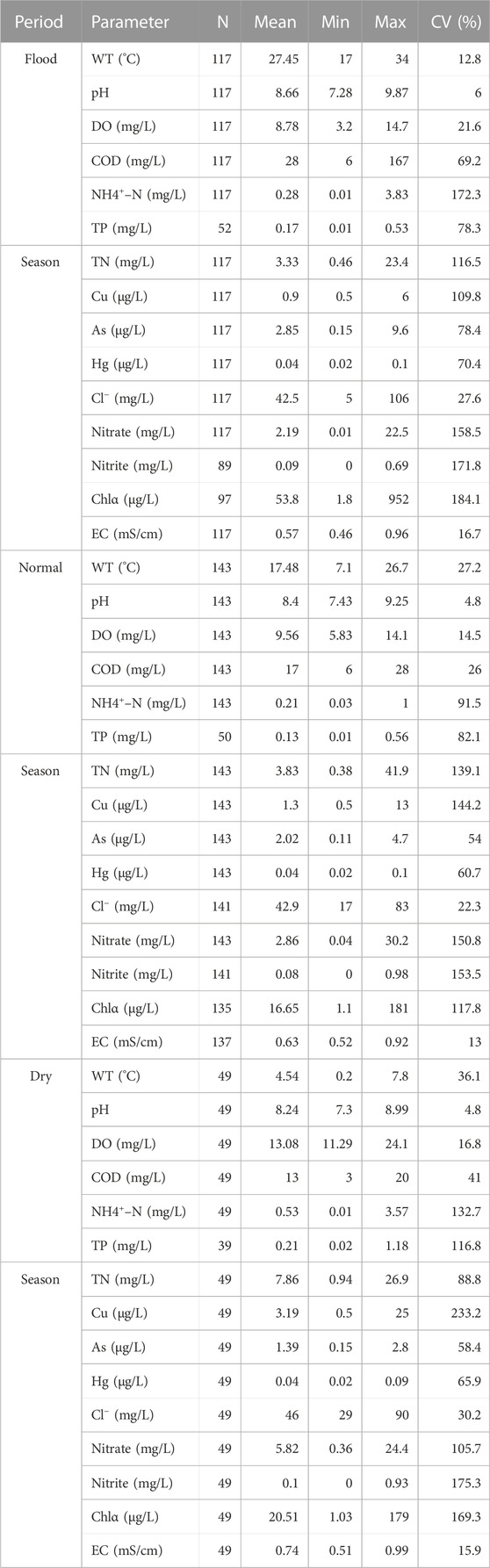
TABLE 1. Temporal changes of the physicochemical parameters in the study area.

The standard deviations suffered from the problem of having different dimensions for different parameters. To resolve this issue, the CV was introduced. If the CV > 100%, the dataset had a large dispersion. The CVs of TN, NH₄⁺–N, nitrate, nitrite, and chlα were >100% in each season, meaning that the nitrogen matters were highly diverse in different locations of the watershed. The remainder of the parameters had acceptable CVs. The problem was that some organic and biological matters had increased above an acceptable level.

It was shown that the average values of WT in the upstream area, at the reservoir, and in the downstream area were 17.32, 20.73, and 19.79°C, respectively. The average levels of DO were 10.27, 9.41, and 9.97 mg/L, respectively. Meanwhile, the average EC values for these locations were 0.7, 0.57, and 0.6 m/cm, respectively. The values of COD in the reservoir and downstream had a range of 16.2–28.3 mg/L, which were similar; the upstream COD ranged from 9.4 to 16.8 mg/L. About 1 mg/L of TN was recorded both at the reservoir and in the downstream area, which was different from the upstream area, which had a range of 4.26–11.9 mg/L for TN. Therefore, the TN Q_i values at the upstream area were 400–1,000, which were higher than those in the other places. The sub-indices at the upstream area were 20–60, which occupied a relatively large proportion of the WQI scores. There were no data for TP at the reservoir, and the TP range was broader in the upstream compared to the downstream areas. The concentrations of Hg were almost safe in the watershed (0.02–0.1 μg/L). The water body of the reservoir had a higher chlα than the rivers connected with it. The upstream area had a wider range (35–57 mg/L) of Cl⁻ than the other places (40–43 mg/L) (Supplementary Figure S3). The CVs of NH₄⁺–N, TP, Cu, and chlα in the upstream area were >100%, and the values of Cu, nitrate, nitrite, and chlα both at the reservoir and in the downstream were >100% (Table 2). In summary, it was significant that the water condition of the downstream was closer to the water body of the reservoir.

TABLE 2

TABLE 2. Temporal changes of the physicochemical parameters in the study area.

To conclude, the WQI showed that the water quality in this watershed was normal in general, but the content of COD, TN, and chlα was in a terrible state. Most parameters were time independent, except for the three (WT, DO, and EC) used for clustering in different seasons. The influence of the Yuqiao Reservoir caused the downstream area to have a similar content of surface water elements.

3.2 Pollution source identification using PCA/FA

The datasets that were suitable for the approach of PCA/FA should have the necessity of adjusting three guidelines: >0.5 for the KMO quantity, >100 for chi-square, and <0.05 for the significance criteria. The KMO quantities for the FS, NS, and DS were 0.603, 0.593, and 0.579, respectively. The chi-square values of the FS, NS, and DS were 238.267, 321.518, and 331.56, respectively. The statistical significances of the FS, NS, and the DS were all 0.000. All of the datasets were suitable for performing pollution source analysis.

A total of 15 parameters were used to assist in source identification. Six VFs were extracted, having eigenvalues >1 in FS, NS, and DS. The absolute factor loading values are between −1 and 1. Negative numbers represent negative correlations, and the closer the absolute value is to 1, the greater the correlation between the factor and the parameter. The terms “strong,” “moderate,” and “weak” loadings were used for describing factor loadings with absolute factor-loading values > 0.75, 0.75–0.5, and 0.5–0.3, respectively (Su et al., 2011; Yang et al., 2013). Notably, the six factors only explain about 78.2% of the total variance in the FS, 73.5% in the NS, and 81.2% in the DS, which is relatively low. To bolster these values, we added an additional VF representative of the largest portion of the remaining part. In the end, three sets of models had seven factors, which explained about 84.4% of the total variance in the FS, 79.7% in the NS, and 86.4% in the DS. Supplementary Tables S4, S6 show the VFs that were initially extracted and the modified results.

In the flood season, VF1 showed strong positive loadings on TN, nitrate, and nitrite, while moderate negative loadings were evident for pH and As. This VF explained 21.5% of the total variance, implying that this type of pollution had mixed types of organic and metallic matter. Previous studies have indicated that the emission of domestic sewage might cause a variety of organic and metallic components to increase in the surface water (Yang et al., 2013; Qin et al., 2020). As this VF had accounted for the largest proportion, and the land-use type around the reservoir was that of towns and villages, VF1 was interpreted as the rural domestic pollution source. VF2 showed strong positive loadings on Cl⁻ and EC and moderate positive loadings on NH₄⁺–N, which explained 14.0% of the total variance. Given that the concentration of Cl⁻ and EC in this reservoir was at the level expected of freshwater, this kind of inorganic salt ion might come from the weathering and deposition of rocks, which was imported from the inflow of natural upstream bodies of water. Above all, VF2 was defined as the upstream water source. VF3 explained 12.6% of the total variance. It showed strong positive loadings on COD and chlα, which is representative of the nutrients in the water. The rural domestic pollution source had been defined, so we defined VF3 as the urban domestic pollution source. VF4 explained 12.4% of the total variance, which showed strong positive loadings in DO, moderate positive loadings in pH, and moderate negative loadings in NH₄⁺–N. This component represents another kind of organic pollution whose representative pollutant was NH₄⁺–N. Ammonia nitrogen, as an ingredient, was commonly found in sewage or fertilizer effluent in this watershed (Xu et al., 2015; Gholizadeh Haji et al., 2016). We named the VF4 the fertilizer application pollution source. VF5 showed strong positive loadings on WT, with moderate negative loadings on TP. This VF explains 9.0% of the total variance. The change in weather was a key factor governing the WT. When rain fell, the cooling of the atmosphere and the injection of rain caused the water temperature to fall and caused the runoff of the arable land to increase, which was rich in phosphorus. Therefore, VF5 was defined as the seasonal factor influence source. VF6 showed strong positive loadings in Hg and close to moderate positive loadings on As, which explained 8.1% of the total variance. This is a typical type of heavy-metal pollution usually associated with industrial emissions in aquatic ecosystems (Liu et al., 2019b). Hence, the industrial pollution source was defined for the FS. Last, VF7 showed strong positive loadings only on Cu, which explained 6.8% of the total variance. As Cu is often associated with vehicle exhaust and broken cars (Yang et al., 2013), VF7 was defined as the vehicle exhaust emission pollution source.

In the normal season, VF1 showed strong positive loadings on TN and nitrate, while moderate positive loadings were observed on nitrite. This VF explained 17.0% of the total variance. In previous studies, pollutants associated with the nitrate/nitrate ratio described previously typically appear in polluted water in villages (Zheng et al., 2015; Qin et al., 2020). VF1 was defined as the rural domestic pollution source. VF2 showed strong positive loadings on Cl⁻ and moderate positive loadings on EC and NH₄⁺–N, which explains 13.9% of the total variance. We defined this as the upstream water source because it was similar to VF2 in the flood season. VF3 showed strong positive loadings on the metal element, As, and moderate positive loadings on COD (12.6%). Defining this as the industrial pollution source was reasonable since the organic pollutant could also have occurred in industrial wastewater. VF4 explained 10.8% of the total variance. It showed strong positive loadings on WT, moderate positive loadings on pH, and moderate negative loadings on DO. In this way, VF4 mainly reflected the change in water temperature, so it was regarded as the seasonal factor influence source. VF5 showed strong positive loadings on Hg and moderate positive loadings on NH₄⁺–N. This VF explained 10.1% of the total variance. The industrial pollution source had been defined with VF3, so we considered that VF5 was more likely the fertilizer application pollution source because some kinds of chemical fertilizer also contained trace amounts of metal. VF6 showed strong positive loadings on Cu and moderate positive loadings on pH, which explained 7.9% of the total variance. That meant this varifactor was similar to VF7 in the FS, which was the vehicle exhaust emission pollution source. VF7 explained 7.4% of the total variance, which showed strong positive loadings on chlα. This is representative of a type of organic pollution, so it was defined as the rural domestic pollution source.

In the dry season, VF1 explained 23.6% of the total variance, as it showed strong positive loadings on four types of parameters: NH₄⁺–N, TN, As, and nitrate. Three of them were related to nitrogen and the nutrients it represented. The rural domestic pollution source was attributed to VF1. VF2 showed strong positive loadings on COD and moderate positive loadings on DO and chlα, which explained 13.0% of the total variance. As a source of organic pollution caused by urban activities, it was believed that VF2 should be attributed to the urban domestic pollution source. VF3 explained 12.9% of the total variance and showed strong positive loadings on Cl⁻ and nitrite, which meant this was a source of natural inorganic ions. As such, this was defined as the upstream water source. VF4 showed strong positive loadings on the fertilizer components of NH₄⁺–N and TP (10.7%). Defining this as fertilizer application pollution was available and seemingly appropriate, according to the previous study of this area (Zhang et al., 2003). VF5 showed strong negative loadings on Cu and explained 9.4% of the total variance. It was necessary to name this the vehicle exhaust emission pollution source. VF6 explained 8.9% of the total variance, which showed strong positive loadings only on WT, and we considered it to be the seasonal factor influence source. VF7 explained 7.9% of the total variance, which was more concentrated on the metal element of Hg, justifying why we assigned the dry season VF7 as the industrial pollution source.

In summary, seven main pollution sources were extracted. These included urban districts, rural districts, industry, weather, fertilizer, upstream, and vehicle. VFs representing organic pollution, such as the urban and rural districts, and fertilizer erosion usually explained a greater percentage of variance.

3.3 Source apportionment using absolute principal component score–multiple linear regression model

After identifying the main pollution sources during the process of PCA/FA, the APCS–MLR model was used for discharging the apportionment of each pollution source in different seasons. The percentage of different sources of pollution for the 15 parameters in flood, normal, and dry seasons are shown in Tables 3–5. The metric A-R² represents the fitting effect of this model’s description. In the flood season, the top three pollution sources were the upstream water source (UWS, 26.6%), the urban domestic pollution source (UDPS, 21.5%), and the vehicle emission pollution source (VEPS, 10.9%). In the normal season, the top three were the upstream water source (22.3%), the rural domestic pollution source (RDPS, 19.8%), and the fertilizer application pollution source (FEPS, 15.8%). In the dry season, the top three belonged to the upstream water source (26.4%), the urban domestic pollution source (19.0%), and the fertilizer application pollution source (18.8%). Some of the parameters had relatively stable relationships with a series of pollution sources. The rural domestic pollution source (RDPS) was strongly related to TN (61.8%, FS; 56.6%, NS; 59.0%, DS) and nitrate (68.9%, FS; 56.7%, NS; 60.1%, DS) in each season. The UWS) was connected with Cl⁻ (59.1%, FS; 61.4%, NS; 42.2%, DS) and EC (44.5%, FS; 29.7%, NS). The UDPS provided a large proportion of chlα (80.4%, FS; 60.4%, NS; 30.7%, DS). The FEPS was mainly represented by NH₄⁺–N (37.2%, FS; 18.3%, NS; 31.2%, DS) and TP (28.4%, NS; 52.8%, DS). The seasonal factor influence source (SFIS) had a close relationship with the natural pattern of WT (53.2%, FS; 62.0%, NS; 47.8%, DS). The industrial pollution source (IPS) had a strong positive correlation with at least one of the two heavy-metal elements, As (19.3%, FS; 40.8%, NS) and Hg (69.9%, FS; 61.4%, DS). The VEPS was evidently related to Cu (80.3%, FS; 55.9%, NS; 48.8%, DS). The source of other parameters was diverse in different seasons. The main influential factors of pH, an indicator of measuring how acidic or alkaline water is, are villages during the FS (25.0%), vehicle emissions (21.2%), weather in the NS (24.8%), and urban in the DS (30.8%). The DO and COD represent the physicochemical index of water. Their main influence factors were urban (COD, 56.2%) and fertilizer (DO, 54.9%) in the FS, temperature (DO, 18.8%) and industry (DO, 16.2%; COD, 30.3%) in the NS, and urban (DO, 45.4%) and villages (COD, 43.8%) in the DS. It seemed that upstream was the first factor (21.7%, FS) of nitrite at first; then, it changed to the influence of villages (20.8%, NS), and then, it came from upstream (38.2%, DS) again. However, nitrogen transformation processes in this region will require more discussion concerning future source locations of nitrogen pollution. The source of heavy-metal elements experienced some subtle changes: industry was dominant (19.3%, As; 69.9%, Hg) in the FS; in the NS, however, fertilizer provided the largest proportion of Hg (55.9%); at last, villages provided 38.5% of As and industry provided 61.4% of Hg, both of which occurred in the DS. The upstream pollution was mostly considered to contribute the highest proportion in all three seasons (26.6%, FS; 22.3%, NS; 26.4%, DS). The second highest proportion was urban pollution in both the FS and the DS (21.5%, FS; 19.0%, DS) and rural pollution (19.8%) in the NS. The conditions of total average contribution in different seasons are shown in Figure 5. It shows that the pollution distribution rates from the urban area (21.5%, FS), upstream (26.6%, FS), and industry (9.4%, FS) in the flood season were higher than those in the other seasons; the distributions from the fertilizer (18.8%, DS) and the seasonal factor (12.9%, DS) in the dry season were more than the others, and the villages (19.8%, NS) and the vehicle erosion (12.5%, NS) in the normal season had larger proportions than the others (Supplementary Figure S4). Above all, it was shown that upstream pollution from living activities in both urban and rural areas was the dominant factor.

TABLE 3

TABLE 3. Contribution of pollution sources for each pollutant in the flood season with PCA/FA results.

TABLE 4

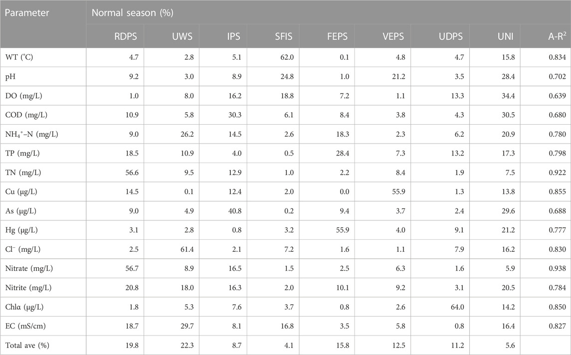
TABLE 4. Contribution of pollution sources for each pollutant in the normal season with PCA/FA results.

TABLE 5

TABLE 5. Contribution of pollution sources for each pollutant in the dry season with PCA/FA results.

3.4 Source apportionment using the PMF model

Eight factors had been set up in the flood season, the normal season, and the dry season. One factor for each season is to be chosen as the unidentified source (UNI). Figure 3 shows the “Factor Figureprints” of all analyzed variables resulting from the EPA PMF model in the flood, normal, and dry seasons. The rules for defining factors extracted by the PMF method were the same as when we defined the other factors extracted by the PCA/FA method, such as linking chlα with the urban pollution source, TN, and nitrate with the rural source; we hung the fertilizer source on the factor close to NH₄⁺–N and tied the vehicle emission source to the element Cu. There were a few exceptions. One of the sources in the flood season mostly consisted of Hg but not Cu, which was defined as the vehicle emission pollution source, as we should put the source of urban and villages into the true position in advance. There were no seasonal factors in the flood and normal seasons and no vehicle emission source in the dry season. Nitrite was an abandoned factor because it was less important in comparison with the other water parameters.

FIGURE 3

FIGURE 3. Factor figureprints of 24 studied variables resulting from the EPA PMF model in the FS, NS, and DS (LBPS, livestock breeding pollution source; NO3_N, nitrate; NO2_N, nitrite).

The contribution of these factors is shown in Supplementary Figure S5. Average contributions indicated that RDPS, FEPS, LBPS, UDPS, IPS, VEPS, UWS, and UNI for different variable concentrations in the flood season were 11.2%, 9.2%, 13.8%, 12.5%, 16.1%, 12.8%, 15.4%, and 9.1%, respectively. The RDPS, FEPS, LBPS, UDPS, IPS, VEPS, UWS, and UNI for different variable concentrations in the normal season were 10.5%, 11.8%, 15.1%, 12.4%, 14.2%, 9.4%, 16.3%, and 10.2%, respectively. Meanwhile, the average contributions of RDPS, FEPS, LBPS, UDPS, IPS, SFIS, UWS, and UNI for different variable concentrations in the dry season were 14.5%, 10.1%, 12.0%, 10.0%, 13.3%, 14.2%, 15.6%, and 10.2%, respectively. The contribution of each factor in the PMF model was relatively average, but the proportion seems to be larger, again, in the pollution from upstream, rural living, and industrial activities, according to the PMF results.

3.5 The comparison of APCS–MLR and PMF models

The comparison of the obtained results of PMF and APCS–MLR models is graphed in Figure 4. Some differences in identifying the sources in the same dataset are evident. The first step is to determine whether a difference exists. The APCS–MLR model shows that the seasonal factor existed in all months, but the PMF model suggests that it was present only in the dry season. In contrast, the LBPS was a unique exception to the PMF model, which the APCS–MLR model could not identify. Second, there are disagreements that would happen in allocating the contribution of each factor. Explained variances of 26.6% and 21.5% had been assigned to the sources of UWS and UDPS in the APCS–MLR model during the FS, respectively, which was much higher than that in the PMF model (15.4% and 12.5%). Similar things were evident in the source of RDPS and UWS in the normal season and UWS, FEPS, and UDPS in the dry season. In contrast, it was found that contributions in the PMF model were higher than those in the APCS–MLR for IPS and FEPS in the flood season, IPS in the normal season, and RDPS and IPS in the dry season. Overall, the allocation field of the APCS–MLR model was more unbalanced than that of the PMF model.

FIGURE 4

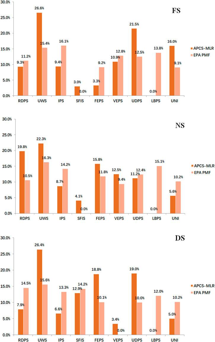
FIGURE 4. Pollution distribution rate in FS, NS, and DS (column graph).

The predicted vs. observed scatter plots from the results of the PMF and APCS–MLR models were analyzed for critical chemical species (Supplementary Figure S6). Three kinds of water parameters were chosen: TN represented the organic materials, Cl⁻represented the non-metallic ions of inorganic materials, and As represented inorganic metallic elements. They showed that the regression results of TN and As in the PMF model were better than those in the APCS–MLR model, and the results for Cl⁻ opposed the trend of the other two parameters. The PMF and APCS–MLR were in agreement in that the source from UDPS, RDPS, and UWS constituted a larger proportion compared with the other pollution sources.

The PMF model demonstrated skill in identifying certain single parameters such as TN and As. However, considering the condition of these datasets, the APCS–MLR model showed a better overall performance. On average, its fitting effects for all parameters were more stable to ensure that R2 > 0.5 was more than that of the PMF model (Figure 5). The PMF had difficulty in establishing a good source resolution for each parameter. The simulation effects of this model on different water quality parameters were so different that R² of two or three parameters was less than 0.5. Most previous studies used the PCA/FA and APCS–MLR, as opposed to the PMF model (Anderson et al., 2002; Gholizadeh Haji et al., 2016). Compared with PMF, the interpretation procedure involved in the APCS–MLR analysis was relatively simple (Guan et al., 2019). As such, APCS–MLR could be a powerful and useful statistical tool when data size and/or quality limit the implementation of PMF (Jain et al., 2018). Above all, we concluded that the APCS–MLR model was the better choice for identifying the source of pollution in the Yuqiao Reservoir.

FIGURE 5

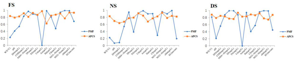
FIGURE 5. Line graphs of R² values in FS, NS, and DS using the APCS–MLR and EPA PMF methods.

4 Conclusion

It was significant from the dataset of 15 parameters at 10 sampling sites that the water quality was generally adequate; still, the problem of eutrophication existed as evidenced by the concentrations of COD, TN, TP, and chlα. Three seasonal divisions called FS, NS, and DS were extracted by the cluster analysis method, and PCA/FA was used to extract seven factors for each season’s data. The local water pollution sources were summarized into seven types: fertilizer erosion, urban district pollution, vehicle emissions, industrial pollution, rural district pollution, seasonal factor, and upstream water sources. According to the APCS–MLR model, the pollution source that ranked first was the rural district pollution source for all seasons, and the pollution from upstream was ranked second. Urban sources ranked low in the NS, fertilizer sources ranked low in the FS, vehicle emission sources ranked low in the DS, and sources attributed to villages ranked high in the NS. It was found that the PMF model allocated an even proportion to each source of pollution. The upstream source always ranked first or second for each season in the PMF model. The proportion of upstream sources was usually high in both the APCS–MLR and PMF models, and the seasonal factor was more evidently pronounced in the DS than in the other seasons. R² results indicated that the APCS–MLR model performed better in the entirety of the study.

The main factors of the water pollution in the Yuqiao Reservoir in 2015–2016 were upstream, urban, and rural sources. To reduce the pollution level of the reservoir, removing nitrogen and phosphorus nutrients from local and upstream rural domestic sewage is key to domestic water pollution control. This study could help local governments establish guidelines and inspire watershed and surface water pollution control measures. The Ministry of Ecology and Environment should take actions in building rural and eutrophic treatment facilities to address the impact of livestock and poultry breeding wastewater. Measures related to completing the coverage of urban production and living sewage treatment, promoting local control of chemical fertilizer use, treating industrial wastewater, monitoring vehicle exhaust emissions, etc., are also necessary. Future research is needed for 1) focusing on the pollution sources of nutrients and organic matter through the use of statistical methods, and 2) the results of the mathematical model study were compared with those of the isotope correlation study.

Data availability statement

The data analyzed in this study are subject to the following licenses/restrictions: The datasets analyzed during the current study are not publicly available due to the restriction of the local water services department but are available from the corresponding author on reasonable request. Requests to access these datasets should be directed to phytoplankton@163.com.

Author contributions

ZW, investigation, writing and original draft; DJ, investigation, writing and original draft, funding acquisition; SS, Investigation; JS, conceptualization, supervision, funding acquisition, writing, review and editing.

Funding

We are grateful to the financial support by the National Natural Science Foundation of China (42006174 and 41876134), and the National Key Research and Development Project of China (2019YFC1407803).

Conflict of interest

The authors declare that the research was conducted in the absence of any commercial or financial relationships that could be construed as a potential conflict of interest.

Publisher’s note

All claims expressed in this article are solely those of the authors and do not necessarily represent those of their affiliated organizations, or those of the publisher, the editors, and the reviewers. Any product that may be evaluated in this article, or claim that may be made by its manufacturer, is not guaranteed or endorsed by the publisher.

Supplementary material

The Supplementary Material for this article can be found online at: https://www.frontiersin.org/articles/10.3389/fenvs.2023.1107591/full#supplementary-material

References

Abbas, F. M. A., Ahmad, A., and Azhar, M. E. (2008). Assessment of surface water quality of selected estuaries of Malaysia: Multivariate statistical techniques. Environ. 29 (3), 255–262. doi:10.1007/s10669-008-9190-4

CrossRef Full Text | Google Scholar

Anderson, M. J., Daly, E. P., Miller, S. L., and Milford, J. B. (2002). Source apportionment of exposures to volatile organic compounds: II. Application of receptor models to TEAM study data. Atmos. Environ. 36, 3643–3658. doi:10.1016/S1352-2310(02)00280-7

CrossRef Full Text | Google Scholar

Aydin, H., Ustaoglu, F., Tepe, Y., and Soylu, E. N. (2021). Assessment of water quality of streams in northeast Turkey by water quality index and multiple statistical methods. Environ. Forensics 22 (1-2), 270–287. doi:10.1080/15275922.2020.1836074

CrossRef Full Text | Google Scholar

Brown, R. M., Mclelland, N. I., Deininger, R. A., and O’Connor, M. F. (1972). A water quality index-crashing the psychological barrier. Indic. Environ. Qual. 1972 (1), 173–182. doi:10.1007/978-1-4684-2856-8_15

CrossRef Full Text | Google Scholar

Brown, S. G., Eberly, S., Paatero, P., and Norris, G. A. (2015). Methods for estimating uncertainty in PMF solutions: Examples with ambient air and water quality data and guidance on reporting PMF results. Sci. Total Environ. 518, 626–635. doi:10.1016/j.scitotenv.2015.01.022

PubMed Abstract | CrossRef Full Text | Google Scholar

Chai, N. P., Yi, X., Xiao, J., Liu, T., Liu, Y., and Deng, L. (2021). Spatiotemporal variations, sources, water quality and health risk assessment of trace elements in the Fen River. Science of the Total Environment 757, 11

CrossRef Full Text | Google Scholar

Chen, R. H., Teng, Y. G., Chen, H. Y., Hu, B., and Yue, W. F. (2019). Groundwater pollution and risk assessment based on source apportionment in a typical cold agricultural region in Northeastern China. Sci. Total Environ. 696, 133972. doi:10.1016/j.scitotenv.2019.133972

PubMed Abstract | CrossRef Full Text | Google Scholar

Cuce, H., Kalipci, E., Ustaoglu, F., Kaynar, I., and Turkmen, M. (2022). Multivariate statistical methods and GIS based evaluation of the health risk potential and water quality due to arsenic pollution in the Kizilirmak River. Int. J. Sediment Res. 37 (6), 754–765. doi:10.1016/j.ijsrc.2022.06.004

CrossRef Full Text | Google Scholar

Enorth.com (2022). Yuqiao reservoir. Available at: http://news.enorth.com.cn/system/2022/06/09/052759103.shtml.

Google Scholar

Fraga, M. D., Reis, G. B., da Silva, D. D., Guedes, H. A. S., and Elesbon, A. A. A. (2020). Use of multivariate statistical methods to analyze the monitoring of surface water quality in the Doce River basin, Minas Gerais, Brazil. Environ. Sci. Pollut. Res. 27 (28), 35303–35318. doi:10.1007/s11356-020-09783-0

PubMed Abstract | CrossRef Full Text | Google Scholar

Fu, D., Wu, X. F., Chen, Y. C., and Yi, Z. Y. (2020). Spatial variation and source apportionment of surface water pollution in the Tuo River, China, using multivariate statistical techniques. Environ. Monit. Assess. 192 (12), 745. doi:10.1007/s10661-020-08706-3

PubMed Abstract | CrossRef Full Text | Google Scholar

Gholizadeh Haji, M., Melesse, A. M., and Reddi, L. (2016). Water quality assessment and apportionment of pollution sources using APCS-3MLR and PMF receptor modeling techniques in three major rivers of South Florida. Sci. Total Environ. 566-567, 1552–1567. doi:10.1016/j.scitotenv.2016.06.046

PubMed Abstract | CrossRef Full Text | Google Scholar

Guan, Q., Zhao, R., Pan, N., Wang, F., Yang, Y., and Luo, H. (2019). Source apportionment of heavy metals in farmland soil of Wuwei, China: Comparison of three receptor models. J. Clean. Prod. 237, 117792. doi:10.1016/j.jclepro.2019.117792

CrossRef Full Text | Google Scholar

Jain, S., Sharma, S. K., Mandal, T. K., and Saxena, M. (2018). Source apportionment of PM10 in Delhi, India using PCA/APCS, UNMIX and PMF. Particuology 37, 107–118. doi:10.1016/j.partic.2017.05.009

CrossRef Full Text | Google Scholar

Kamble, S. R., and Vijay, R. (2011). Assessment of water quality using cluster analysis in coastal region of Mumbai, India. Environ. Monit. Assess. 178 (1-4), 321–332. doi:10.1007/s10661-010-1692-0

PubMed Abstract | CrossRef Full Text | Google Scholar

Li, S. Y., Li, J., and Zhang, Q. F. (2011). Water quality assessment in the rivers along the water conveyance system of the Middle Route of the South to North Water Transfer Project (China) using multivariate statistical techniques and receptor modeling. J. Hazard. Mater. 195, 306–317. doi:10.1016/j.jhazmat.2011.08.043

PubMed Abstract | CrossRef Full Text | Google Scholar

Liu, K., Wang, F., Li, J. W., Tiwari, S., and Chen, B. (2019b). Assessment of trends and emission sources of heavy metals from the soil sediments near the Bohai Bay. Environ. Sci. Pollut. Res. 26, 29095–29109. doi:10.1007/s11356-019-06130-w

PubMed Abstract | CrossRef Full Text | Google Scholar

Liu, L. L., Dong, Y. C., Kong, M., Zhou, J., Zhao, H. B., Tang, Z., et al. (2020). Insights into the long-term pollution trends and sources contributions in Lake Taihu, China using multi-statistic analyses models. Chemosphere 242, 125272. doi:10.1016/j.chemosphere.2019.125272

PubMed Abstract | CrossRef Full Text | Google Scholar

Liu, L. L., Tang, Z., Kong, M., Chen, X., Zhou, C. C., Huang, K., et al. (2019a). Tracing the potential pollution sources of the coastal water in Hong Kong with statistical models combining APCS-MLR. J. Environ. Manag. 245, 143–150. doi:10.1016/j.jenvman.2019.05.066

PubMed Abstract | CrossRef Full Text | Google Scholar

Lu, H. M., and Yin, C. Q. (2008). Shallow groundwater nitrogen responses to different land use managements in the riparian zone of Yuqiao Reservoir in North China. J. Environ. Sci. 20 (6), 652–657. doi:10.1016/S1001-0742(08)62108-7

PubMed Abstract | CrossRef Full Text | Google Scholar

Meng, L., Zuo, R., Wang, J. S., Yang, J., Teng, Y. G., Shi, R. T., et al. (2018). Apportionment and evolution of pollution sources in a typical riverside groundwater resource area using PCA-APCS-MLR model. J. Contam. Hydrology 218, 70–83. doi:10.1016/j.jconhyd.2018.10.005

PubMed Abstract | CrossRef Full Text | Google Scholar

Ministry of Finance of the People's Republic of China (2021). Tianjin went deep into Yuqiao Reservoir research service "three water" people's livelihood construction. Available at: http://www.mof.gov.cn/zhengwuxinxi/xinwenlianbo/tianjingcaizhengxinxilianbo/202106/t20210603_3713979.htm.

Google Scholar

Ministry of Water Resources of the People's Republic of China (2015). China water resource bulletin 2015. Available at: http://www.mwr.gov.cn/sj/tjgb/szygb/201612/t20161229_783348.html (Accessed February 10th, 2022).

Google Scholar

National Meteorological Center of CMA (1981). Monthly mean temperature and precipitation (Jizhou). Available at: http://www.nmc.cn/publish/forecast/ATJ/jizhou.html (Accessed 10th March, 2022).

Google Scholar

Qi, W. Q. (2002). Chapter 3. In: Standard methods for the examination of water and wastewater. 4th edn. Beijing, China, 88–438. (in Chinese).

Google Scholar

Qin, G. S., Liu, J. W., Xu, S. G., and Wang, T. X. (2020). Water quality assessment and pollution source apportionment in a highly regulated river of Northeast China. Environ. Monit. Assess. 192 (7), 446. doi:10.1007/s10661-020-08404-0

PubMed Abstract | CrossRef Full Text | Google Scholar

Rafighdoust, Y., Eckstein, Y., Harami, R. M., Gharaie, M. H. M., and Mahboubi, A. (2016). Using inverse modeling and hierarchical cluster analysis for hydrochemical characterization of springs and Talkhab River in Tang-Bijar oilfield, Iran. Arabian J. Geosciences 9 (3), 241. doi:10.1007/s12517-015-2129-4

CrossRef Full Text | Google Scholar

Shrestha, S., Kazama, F., and Nakamura, T. (2008). Use of principal component analysis, factor analysis and discriminant analysis to evaluate spatial and temporal variations in water quality of the Mekong River. J. Hydroinformatics 10, 43–56. doi:10.2166/hydro.2008.008

CrossRef Full Text | Google Scholar

Singh, K. P., Malik, A., and Sinha, S. (2005). Water quality assessment and apportionment of pollution sources of Gomti river (India) using multivariate statistical techniques - a case study. Anal. Chim. Acta 538 (1-2), 355–374. doi:10.1016/j.aca.2005.02.006

CrossRef Full Text | Google Scholar

Soltani, A. A., Bermad, A., Boutaghane, H., Oukil, A., Abdalla, O., Hasbaia, M., et al. (2020). An integrated approach for assessing surface water quality: Case of Beni Haroun dam (Northeast Algeria). Environ. Monit. Assess. 192 (10), 630. doi:10.1007/s10661-020-08572-z

PubMed Abstract | CrossRef Full Text | Google Scholar

State Environmental Protection Administration (2002). The national standards of the people s Republic of China: Environmental quality standards for surface water (GB3838-2002). Beijing, China: State Environmental Protection Administration.

Google Scholar

Su, J., Qiu, Y. H., Lu, Y. L., Yang, X. S., and Li, S. Y. (2021). Use of multivariate statistical techniques to study spatial variability and sources apportionment of pollution in rivers flowing into the laizhou bay in dongying district. Water 13 (6), 772. doi:10.3390/w13060772

CrossRef Full Text | Google Scholar

Su, S. L., Li, D., Zhang, Q., Xiao, R., Huang, F., and Wu, J. P. (2011). Temporal trend and source apportionment of water pollution in different functional zones of Qiantang River, China. Water Res. 45 (4), 1781–1795. doi:10.1016/j.watres.2010.11.030

PubMed Abstract | CrossRef Full Text | Google Scholar

Thurston, G. D., and Spengler, N. D. (1985). A quantitative assessment of source contributions to inhalable particulate matter pollution in metropolitan Boston. Atmos. Environ. 19, 9–25. doi:10.1016/0004-6981(85)90132-5

CrossRef Full Text | Google Scholar

Topaldemir, H., Tas, B., Yuksel, B., and Ustaoglu, F. (2022). Potentially hazardous elements in sediments and ceratophyllum demersum: An ecotoxicological risk assessment in milic wetland, samsun, Turkiye. Environ. Sci. Pollut. Res. 20. doi:10.1007/s11356-022-23937-2

CrossRef Full Text | Google Scholar

Ustaoglu, F., Tas, B., Tepe, Y., and Topaldemir, H. (2021). Comprehensive assessment of water quality and associated health risk by using physicochemical quality indices and multivariate analysis in Terme River, Turkey. Environ. Sci. Pollut. Res. 28 (44), 62736–62754. doi:10.1007/s11356-021-15135-3

CrossRef Full Text | Google Scholar

Ustaoglu, F., Tepe, Y., and Tas, B. (2020). Assessment of stream quality and health risk in a subtropical Turkey river system: A combined approach using statistical analysis and water quality index. Ecol. Indic. 113, 105815. doi:10.1016/j.ecolind.2019.105815

CrossRef Full Text | Google Scholar

Ustaoglu, F., and Tepe, Y. (2019). Water quality and sediment contamination assessment of Pazarsuyu Stream, Turkey using multivariate statistical methods and pollution indicators. Int. Soil Water Conservation Res. 7 (1), 47–56. doi:10.1016/j.iswcr.2018.09.001

CrossRef Full Text | Google Scholar

Vega, M., Pardo, R., Barrado, E., and Deban, L. (1998). Assessment of seasonal and polluting effects on the quality of river water by exploratory data analysis. Water Res. 32 (12), 3581–3592. doi:10.1016/S0043-1354(98)00138-9

CrossRef Full Text | Google Scholar

Wang, X. H., Yin, C. Q., and Shan, B. Q. (2004). Control of diffuse P-pollutants by multiple buffer/detention structures by Yuqiao Reservoir, North China. J. Environ. Sci. 04, 616–620. doi:10.3321/j.issn:1001-0742.2004.04.018

PubMed Abstract | CrossRef Full Text | Google Scholar

Wang, Y., Wang, P., Bai, Y. J., Tian, Z. X., Li, J. W., Shao, X., et al. (2013). Assessment of surface water quality via multivariate statistical techniques: A case study of the songhua river harbin region, China. J. Hydro-Environment Res. 7 (1), 30–40. doi:10.1016/j.jher.2012.10.003

CrossRef Full Text | Google Scholar

World Health Organization (2011). Guidelines for drinking water quality. Available at: https://www.who.int/teams/environment-climate-change-and-health/water-sanitation-and-health/chemical-hazards-in-drinking-water.

Google Scholar

Wu, J. D., and Peng, Z. L. (2016). Tianjin statistical yearbook 2016 and Tianjin statistical yearbook 2017, Tianjin Bureau of statistics. Available at: http://stats.tj.gov.cn/nianjian/2016nj/zk/indexch.htm.

Google Scholar

Xu, Y., Xie, R. Q., Wang, Y. Q., and Sha, J. (2015). Spatio-temporal variations of water quality in Yuqiao reservoir basin, north China. Front. Environ. Sci. Eng. 9 (4), 649–664. doi:10.1007/s11783-014-0702-9

CrossRef Full Text | Google Scholar

Yang, L., Mei, K., Liu, X., Wu, L., Zhang, M., Xu, J., et al. (2013). Spatial distribution and source apportionment of water pollution in different administrative zones of Wen-Rui-Tang (WRT) river watershed, China. Environ. Sci. Pollut. Res. 20 (8), 5341–5352. doi:10.1007/s11356-013-1536-x

PubMed Abstract | CrossRef Full Text | Google Scholar

Yuksel, B., and Arica, E. (2018). Assessment of toxic, essential, and other metal levels by ICP-ms in lake eymir and mogan in ankara, Turkey: An environmental application. At. Spectrosc. 39 (5), 179–184. doi:10.46770/AS.2018.05.001

CrossRef Full Text | Google Scholar

Zhang, H., Li, H. F., Yu, H. R., and Cheng, S. Q. (2020). Water quality assessment and pollution source apportionment using multi-statistic and APCS-MLR modeling techniques in Min River Basin, China. Environ. Sci. Pollut. Res. 27 (33), 41987–42000. doi:10.1007/s11356-020-10219-y

PubMed Abstract | CrossRef Full Text | Google Scholar

Zhang, S. R., Chen, L. D., Fu, B. J., and Li, J. R. (2003). The risk assessment of nonpoint pollution of phosphorus from agricultural lands: A case study of Yuqiao reservoir. Watershed 23 (3), 262–269. doi:10.3321/j.issn:1001-7410.2003.03.004

CrossRef Full Text | Google Scholar

Zhao, Y., Nan, J., Cui, F. Y., and Guo, L. (2007). Water quality forecast through application of BP neural network at Yuqiao reservoir. J. Zhejiang University-Science A 8 (9), 1482–1487. doi:10.1631/jzus.2007.a1482

CrossRef Full Text | Google Scholar

Zheng, L. Y., Yu, H. B., and Wang, Q. S. (2015). Assessment of temporal and spatial variations in surface water quality using multivariate statistical techniques: A case study of nenjiang River basin, China. J. Central South Univ. 22 (10), 3770–3780. doi:10.1007/s11771-015-2921-z

CrossRef Full Text | Google Scholar

Zhou, F., Huang, G. H., Guo, H. C., Zhang, W., and Hao, Z. J. (2007). Spatio-temporal patterns and source apportionment of coastal water pollution in eastern Hong Kong. Water Res. 41 (15), 3429–3439. doi:10.1016/j.watres.2007.04.022

PubMed Abstract | CrossRef Full Text | Google Scholar