High-dimensional CoVaR risk spillover network from oil market to global stock markets—Lessons from the Kyoto Protocol

This paper explores the impact of the Kyoto Protocol by investigating the correlation and risk spillover between the crude oil market and the stock markets of 28 countries during its two commitment periods. Besides time-varying Copula-CoVaR models, the Adaptive Lasso-VAR model with oracle properties is employed in generalized variance decomposition, and a risk connectedness network is constructed to explore risk spillovers between the stock markets of various countries when the crude oil market is at risk. The results reveal positive correlations between the crude oil market and stock markets, which become weaker in the second commitment period than in the first. The crude oil market has both upside and downside spillover effects to most stock markets during both commitment periods, and the upside risk spillover effect is stronger than the downside effect. Overall, most non-signatories of the Kyoto Protocol are net receivers of risk spillovers when the crude oil market is at risk, while most signatories are net exporters of risk spillovers.

1 Introduction

On 13 November 2021, the 26th conference of the United Nations Framework Convention on Climate Change (UNFCCC) adopted the Glasgow Climate Agreement and formulated the implementation details of the Paris Agreement, including market mechanisms, transparency, and time frame. As an early exploration prior to the Paris Agreement, the Kyoto Protocol provided a valuable reference for it in terms of cooperation mechanisms and emission reduction methods, making a significant contribution to the reduction of greenhouse gas emissions (Ma, 2012). Analyzing the data of G7 countries from 2010 to 2019 with a GMM-PVAR model, Dogan et al. (2022) show that the Kyoto Protocol has a significant positive impact on energy transition. Maamoun (2019) uses the generalized synthetic control method (GSCM) to compare the emissions of industrialized countries participating in the Kyoto Protocol with their expected emissions had they not participated, and shows that the actual emissions are reduced by about 7% compared to the expected emissions under the “No-Kyoto” scenario. Specifically, the Kyoto Protocol encourages non-signatories to reduce carbon dioxide emissions while limiting carbon emissions of signatories by establishing cooperation mechanisms such as the joint implementation mechanism, the international emissions trading mechanism, and the clean development mechanism (Kuriyama and Abe, 2018; Tran, 2022).

The Kyoto Protocol includes two commitment periods, 2008–2012 and 2013–2020. Compared to the first commitment period, the legal effect and emission reduction efforts of the second commitment period are weakened, but the target adjustment mechanism is improved. The first commitment period has internationally legal binding force on all signatories, while the legal effect of the second commitment period has some uncertainty. To ensure the implementation of the second commitment period on track, the Doha World Climate Conference in 2012 proposed that the signatories should implement the emission reduction tasks as soon as possible in accordance with relevant laws that provisionally apply before completing the ratification. The emission reduction in the second commitment period is weaker, mainly because the signatories were struggling during the economic downturn post the global financial crisis so that greenhouse gas emissions slowed down accordingly. However, with the recovery of the economy, the emissions rebounded, which put pressure on signatories’ deep emission reduction. In terms of the target adjustment mechanism, the second commitment period differs in flexible mechanisms and applicable qualifications. The signatories had a large quantity of assigned amount unit (AAU), emission reduction unit (ERU), and certified emission reduction (CER) from the first commitment period that need to be carried forward to the second commitment period. Meanwhile, some signatories did not undertake quantitative emission reduction or set emission targets during the second commitment period.

It has been documented that financial development and carbon dioxide emissions in many countries are positively correlated (Jamil et al., 2022; Khan et al., 2022). As the pioneering legal instrument in human history to limit greenhouse gas emissions, the Kyoto Protocol attempts to explore a compromise path between economic growth and environmental protection on a global scale (Depledge, 2022). However, the Kyoto Protocol has also received criticism. In particular, the exclusion of developing countries from emissions targets has been portrayed as a fatal design flaw, and the countries’ legal obligations differ under the principle of “common but differentiated responsibilities” (Maamoun, 2019; Tran, 2022). Nevertheless, the Kyoto Protocol restricts the carbon dioxide emissions through its unique cooperation mechanisms and emission reduction methods (Madaleno and Moutinho, 2017; Mohammed, 2020). Did enterprises improve their green technologies and pursue technological transformation, thereby reducing dependence on crude oil? In the meantime, as the financial property of crude oil becomes increasingly apparent, many investors trade oil as a financial asset (Mensi et al., 2017). The price fluctuation of crude oil inevitably affects enterprises’ production costs as well as investing and financing decisions, which are reflected in the stock market. Does the implementation of the first and second commitment periods of the Kyoto Protocol reduce the risk spillover from the crude oil market to stock markets? Which countries’ stock markets are the main receivers of risk spillovers, and which are the exporters, when the oil market is at risk? This paper provides some answers to these questions.

There has been a large body of research regarding the correlation between crude oil market and stock market. On the one hand, some scholars argue for a negative correlation between the two markets, because higher crude oil prices would reduce current and expected profits, leading to a decline in stock prices. For example, Raza et al. (2016) find with a non-linear ARDL model that crude oil prices have a negative impact on the stock markets of emerging economies, which are vulnerable to extreme events. Maghyereh and Abdoh (2022) reveal that extreme oil price shocks have a negative impact on the stock markets of major oil exporters. On the other hand, many scholars believe that the crude oil market and the stock market should have a positive correlation. Kilian and Park (2009) argue that the rising oil prices in the context of global economic expansion will have a sustained positive impact on stock returns. This is because innovations in the global business cycle stimulate the economy, increasing business demand for industrial commodities, thereby driving up oil prices. Working with an ARJI-EGARCH model, Zhang and Chen (2011) find that the Chinese stock market is correlated with the expected volatility of international oil prices, and that international oil prices have a weak positive impact on the Chinese stock market. Alamgir and Amin (2021) investigate the relationship between the crude oil market and stock market indexes in four south Asian countries using a Non-linear Autoregressive Distributed Lag model and report positive correlations. Among the differentiating factors or angles provided in literature regarding the impact of crude oil market on stock markets are the type and timing of oil shocks, the credit status of a country’s economy, and the oil importer or exporter status of a country (Arampatzidis et al., 2021; Jiang et al., 2021; Ramos & Veiga, 2013).

As the dominant commodity with both consumptive and financial attributes, crude oil represents a risk contagion factor to the financial system (Liu et al., 2022). Therefore, the correlation between international crude oil market and stock markets is often accompanied by risk spillover effects. Studying the correlation and risk spillover effects between the two will not only help investors optimize investment portfolios, but also help financial regulators prevent risk contagion between crude oil and stock markets. Zhang and Ma (2019) study the risk spillover effect between the crude oil market and the stock markets of United States, United Kingdom, and Japan based on the EVaR method, and the results show significant two-way spillover effects. Xu et al. (2019) investigate volatility spillovers between crude oil and stock markets using spillover directional measures and asymmetric spillover measures. Using the VAR for VaR approach, Wen et al. (2019) conclude that risk spillovers are stronger after the 2008 financial crisis than before the crisis.

In order to measure the correlation between the crude oil and stock markets and the associated risk spillover effects, researchers often use the time-varying Copula-CoVaR model with non-linear and asymmetric characteristics in empirical analysis. Working on stock market data of U.S., United Kingdom, E.U. and the BRICS countries with the time-varying Copula model, Reboredo and Ugolini (2016) find that the extreme impact of the crude oil market on stock markets before the financial crisis is smaller than that after the crisis. Ji et al. (2020) use the VAR model and the time-varying Copula-GARCH model to measure the dynamic dependencies and risk spillovers between the BRICS stock markets and the crude oil market. Their results show that oil demand shocks pose significant spillover risks to stock returns.

In recent years, with the rapid development of complex network theory in energy economics research, network analysis has become an important tool for studying the correlation between the crude oil market and stock markets and financial risk contagion. Huang et al. (2018) employ co-movement matrixes to study the coherence of oil-stock nexuses in an integrated research framework composed by the wavelet coherence and the complex network. Liu et al. (2020) adopt a complex network approach to explore the characteristics and underlying mechanisms of self-similar behaviors in the ccrude oil market. Wang et al. (2022) combine $∆\mathrm{C}\mathrm{o}\mathrm{V}\mathrm{a}\mathrm{R}$ and the cascading failure network model to examine the systemic risk contribution in global stock markets, by quantifying the domino effect caused by tail risk propagation and accumulation. Liu et al. (2022) uses CoVaR to construct the risk spillover index proposed by Diebold and Yilmaz (2012, 2014) to investigate the total, directional, and net risk spillover effects when the crude oil market is in extreme conditions. Diebold and Yilmaz (2012, 2014) propose the risk spillover index based on generalized variance decomposition of the VAR model. The risk spillover index overcomes the traditional VAR model’s dependence on Cholesky factor identification, which often leads to different results due to the order of variables, and extends to applications beyond pairwise association. This spillover index has been applied in several studies. Kang et al. (2017) use a multivariate DECO-GARCH model to study the spillover effect between gold, silver, WTI crude oil, corn, wheat and rice futures markets, and find that the gold and silver futures are risk exporters among the commodities, while the other four markets are recipients of risk spillovers. Via static and dynamic networks, Wang et al. (2017) show that on average the real estate and bank sectors are net exporters of extreme risk spillovers while the insurance and diversified financials sectors are net recipients. To overcome the curse of dimensionality and estimation error in case of many parameters, Demirer et al. (2018) propose employing the Lasso-VAR model. The Lasso-VAR model has been employed by Liu et al. (2022) to study risk spillover effects between the crude oil and G20 stock markets, and by Balcilar et al. (2022) to study volatility spillover effects between 27 emerging stock markets and seven cryptocurrency markets. Although Lasso can mitigate the curse of dimensionality, it does not have Oracle properties. The Adaptive Lasso method proposed by Zou (2006) imposes different degrees of penalty on each parameter so that it enjoys the oracle properties while reducing the errors in model parameter estimation. Ren and Zhang (2013) propose the Adaptive Lasso-VAR model and demonstrate its advantage in fitting and prediction accuracy over the conventional VAR model.

Despite all these studies on the relationship between crude oil and stock markets, none has explored the issue from the perspective of the impact of the Kyoto Protocol. In view of this, this paper examines the relationship between the crude oil market and 28 major stock markets in the world (including 17 signatories and 11 non-signatories). Their correlation and risk spillover effects when the crude oil market is at risk are investigated with a variety of models, including ARMA-TGARCH model, Markov regime switching model, time-varying Copula-CoVaR model, and generalized variance decomposition based on the Adaptive Lasso-VAR model. Our interest is to compare and evaluate the correlation and risk spillovers between the two commitment periods of the Kyoto Protocol. The empirical analyses yield several important findings. First, there are positive correlations between crude oil and stock markets. In comparison, the correlation and the risk spillover effects between the crude oil market and most stock markets in the second commitment period are weaker than in the first. Second, the crude oil market at risk has both upside and downside spillover effects to most stock markets, with the upside risk spillover effect being stronger than the downside effect. Third, non-signatories are generally the net receivers of risk spillovers, while signatories are mostly net exporters of risk spillovers conditional on crude oil market in extreme conditions.

The contribution of this paper is threefold. First, in terms of research methodology, the Adaptive Lasso-VAR model with Oracle properties, new to literature, is applied to generalized variance decomposition. It not only solves the estimation problem of high-dimensional VAR model when constructing the risk spillover network proposed by Diebold and Yilmaz (2012, 2014), but also reduces the estimation error of non-zero parameters. Moreover, Ren and Zhang (2010, 2013) do not integrate parameter estimation of the VAR model and the Adaptive Lasso model in a unified framework. This paper fills this void by describing parameter estimation of the Adaptive Lasso-VAR model in full detail.

Second, in terms of the research question, this paper systematically analyzes risk spillovers between the stock markets of 28 countries when the crude oil market is at risk during the first and second commitment periods of the Kyoto Protocol. This research question has not been fully explored in literature, which has focused mostly on stock markets in selected countries rather than providing a global perspective or comparing the effects in the two commitment periods (Reboredo and Ugolini, 2016; Ji et al., 2020). The Copula-CoVaR model employed in this study can effectively describe the dynamic risk spillover between the crude oil and global stock markets, and the risk spillover network can identify the exporters and importers of risk spillovers.

Third, in terms of the research perspective, both downside and upside risk spillover effects of the crude oil market on stock markets are investigated in this paper, while the literature usually examines downside spillover only (Liu et al., 2022). Investigations from the perspective of both long and short positions reveal evident asymmetry in risk spillovers, with upside spillover being more prominent. The findings provide valuable reference for formulating a financial risk firewall mechanism to prevent outbreak and spread of financial crises.

The rest of the paper proceeds as follows. Section 2 introduces the measures and methodology. Section 3 reports and analyzes the empirical results. Section 4 concludes and makes policy recommendations.

2 Methodologies

2.1 Tail risk measures

Popular measures of tail risk include VaR, ES, and CoVaR. VaR represents the maximum loss of an asset or portfolio in a given duration at the confidence level $1-q$. Most studies focus on the VaR from the perspective of long positions—thus are concerned with extreme price decline in the left tail—while few from the perspective of short positions.

Let $r_{i,t}$ be the return of an asset or portfolio. $Va{R}_{q,t}^{down}$ and $Va{R}_{q,t}^{up}$ represent left and right tails risk respectively, that is, $P\left(r_{i,t}\le Va{R}_{q,t}^{down}\right)=q$ and $P\left(r_{i,t}\ge Va{R}_{q,t}^{up}\right)=q$ (Giot & Laurent, 2003; Reboredo & Ugolini, 2016). VaR can be calculated with parametric methods, Monte Carlo simulation, or historical simulation. Parametric estimation of VaR requires a probability distribution of the asset’s or investment portfolio’s return. Since the distribution of a financial return series usually features a sharp peak and fat tails, the skewed t distribution can describe well financial return series (Hansen, 1994). If a return series follows a skewed t distribution with skewness $\eta$ and degrees of freedom $\nu$, then

$\mathit{V}\mathit{a}{\mathit{R}}_{\mathit{q},\mathit{t}}^{\mathit{d}\mathit{o}\mathit{w}\mathit{n}}={\mathit{\mu }}_{\mathit{i},\mathit{t}}+{\mathit{\sigma }}_{\mathit{i},\mathit{t}}{\mathit{F}}_{\mathit{\eta },\mathit{\upsilon }}^{-\mathbf{1}}\left(\mathit{q}\right)(1)$

$\mathit{V}\mathit{a}{\mathit{R}}_{\mathit{q},\mathit{t}}^{\mathit{u}\mathit{p}}={\mathit{\mu }}_{\mathit{i},\mathit{t}}+{\mathit{\sigma }}_{\mathit{i},\mathit{t}}{\mathit{F}}_{\mathit{\eta },\mathit{\upsilon }}^{-\mathbf{1}}\left(\mathbf{1}-\mathit{q}\right)(2)$

where ${\mu }_{i,t}$ is the conditional mean, ${\sigma }_{i,t}$ is the conditional standard deviation, $F_{\eta ,\upsilon }^{-1}\left(q\right)$ is the q-quantile of the skewed t distribution, and $q$ is the tail probability, which takes the value of .05 in this paper.

VaR only considers the loss of a single asset or portfolio in isolation, and does not assess risk transfer between markets. To address this issue, Adrian & Brunnermeier (2016) propose the concept of conditional VaR, or CoVaR. CoVaR represents the extreme risk value of an asset or portfolio when another related asset or portfolio is at extreme risk at the confidence level $1-p$.

As per the nature of the position—long or short—CoVaR can be specified as the downside conditional value at risk, $CoVa{R}_{p,q,t}^{down}$, or the upside conditional value at risk, $CoVa{R}_{p,q,t}^{up}$:

$\mathit{P}\left({\mathit{r}}_{\mathbf{1},\mathit{t}}\le \mathit{C}\mathit{o}\mathit{V}\mathit{a}{\mathit{R}}_{\mathit{p},\mathit{q},\mathit{t}}^{\mathit{d}\mathit{o}\mathit{w}\mathit{n}}|{\mathit{r}}_{\mathbf{2},\mathit{t}}\le \mathit{V}\mathit{a}{\mathit{R}}_{\mathit{q},\mathit{t}}^{\mathit{d}\mathit{o}\mathit{w}\mathit{n}}\right)=\mathit{p}(3)$

$\mathit{P}\left({\mathit{r}}_{\mathbf{1},\mathit{t}}\ge \mathit{C}\mathit{o}\mathit{V}\mathit{a}{\mathit{R}}_{\mathit{p},\mathit{q},\mathit{t}}^{\mathit{u}\mathit{p}}|{\mathit{r}}_{\mathbf{2},\mathit{t}}\ge \mathit{V}\mathit{a}{\mathit{R}}_{\mathit{q},\mathit{t}}^{\mathit{u}\mathit{p}}\right)=\mathit{p}(4)$

where $r_{1,t}$ and $r_{2,t}$ are the returns of two related assets or portfolios (in this paper, usually $r_{1,t}$ is a stock market index return and $r_{2,t}$ is the crude oil return). Both tail probabilities, $p$ and $q$, are assigned as .05 in this paper.

To describe the joint distribution of $r_{1,t}$ and $r_{2,t}$, a Copula function can be used to connect the marginal distribution of the crude oil market and the marginal distribution of the stock market:

$\mathit{C}\left[{\mathit{F}}_{{\mathit{r}}_{\mathbf{1},\mathit{t}}}\left(\mathit{C}\mathit{o}\mathit{V}\mathit{a}{\mathit{R}}_{\mathit{p},\mathit{q},\mathit{t}}^{\mathit{d}\mathit{o}\mathit{w}\mathit{n}}\right),{\mathit{F}}_{{\mathit{r}}_{\mathbf{2},\mathit{t}}}\left(\mathit{V}\mathit{a}{\mathit{R}}_{\mathit{q},\mathit{t}}^{\mathit{d}\mathit{o}\mathit{w}\mathit{n}}\right)\right]={\mathit{F}}_{{\mathit{r}}_{\mathbf{1},\mathit{t}},{\mathit{r}}_{\mathbf{2},\mathit{t}}}\left(\mathit{C}\mathit{o}\mathit{V}\mathit{a}{\mathit{R}}_{\mathit{p},\mathit{q},\mathit{t}}^{\mathit{d}\mathit{o}\mathit{w}\mathit{n}},\mathit{V}\mathit{a}{\mathit{R}}_{\mathit{q},\mathit{t}}^{\mathit{d}\mathit{o}\mathit{w}\mathit{n}}\right)(5)$

where C is a copula function, and $F_{r_{1,t}}$ and $F_{r_{2,t}}$ are the distribution functions of $r_{1,t}$ and $r_{2,t}$, respectively.

The copula function $C\left(u,v\right)$ is linked to Spearman rank correlation coefficient ${\rho }_s$ as in Eq. (6). The Spearman correlation coefficient can measure the correlation between the crude oil market and stock markets in various countries.

${\mathit{\rho }}_{\mathit{s}}=\mathbf{12}\underset{\mathbf{0}}{\overset{\mathbf{1}}{{\displaystyle \int }}}\underset{\mathbf{0}}{\overset{\mathbf{1}}{{\displaystyle \int }}}\mathit{C}\left(\mathit{u},\mathit{v}\right)\mathit{d}\mathit{u}\mathit{d}\mathit{v}-\mathbf{3}(6)$

Introduced on the basis of static models, dynamic Copula models can characterize the ever-changing interdependence between two markets and predict the joint distribution of asset returns. It has wide applications in asset pricing and financial risk management. Popular dynamic Copula models include time-varying (TV) Normal Copula, TV Student t Copula, TV SJC Copula, TV Plackett Copula, TV Clayton Copula, and TV Gumbel Copula.

Next, upon converting the conditional distribution into the ratio of the joint distribution to the marginal distribution, we use a time-varying Copula function to transform Eqs 3, 4 into Eqs 7, 8, respectively.

$\mathit{C}\left({\mathit{F}}_{{\mathit{r}}_{\mathbf{1},\mathit{t}}}\left(\mathit{C}\mathit{o}\mathit{V}\mathit{a}{\mathit{R}}_{\mathit{p},\mathit{q},\mathit{t}}^{\mathit{d}\mathit{o}\mathit{w}\mathit{n}}\right),\mathit{q}\right)=\mathit{p}\mathit{q}(7)$

$\mathit{q}-{\mathit{F}}_{{\mathit{r}}_{\mathbf{1},\mathit{t}}}\left(\mathit{C}\mathit{o}\mathit{V}\mathit{a}{\mathit{R}}_{\mathit{p},\mathit{q},\mathit{t}}^{\mathit{u}\mathit{p}}\right)+\mathit{C}\left({\mathit{F}}_{{\mathit{r}}_{\mathbf{1},\mathit{t}}}\left(\mathit{C}\mathit{o}\mathit{V}\mathit{a}{\mathit{R}}_{\mathit{p},\mathit{q},\mathit{t}}^{\mathit{u}\mathit{p}}\right),\mathbf{1}-\mathit{q}\right)=\mathit{p}\mathit{q}(8)$

Let$G\left(F_{r_{1,t}}\left(CoVa{R}_{p,q,t}^{down}\right)\right)=C\left(F_{r_{1,t}}\left(CoVa{R}_{p,q,t}^{down}\right),q\right)$, $H\left(F_{r_{1,t}}\left(CoVa{R}_{p,q,t}^{up}\right)\right)=q-F_{r_{1,t}}\left(CoVa{R}_{p,q,t}^{up}\right)+C\left(F_{r_{1,t}}\left(CoVa{R}_{p,q,t}^{up}\right),1-q\right)$, then applying the inverse function and standardizing $r_{i,t}$ yield

${\mathit{F}}_{{\mathit{r}}_{\mathbf{1},\mathit{t}}}\left(\mathit{C}\mathit{o}\mathit{V}\mathit{a}{\mathit{R}}_{\mathit{p},\mathit{q},\mathit{t}}^{\mathit{d}\mathit{o}\mathit{w}\mathit{n}}\right)={\mathit{F}}_{\mathit{\eta },\mathit{\upsilon }}\left(\frac{\mathit{C}\mathit{o}\mathit{V}\mathit{a}{\mathit{R}}_{\mathit{p},\mathit{q},\mathit{t}}^{\mathit{d}\mathit{o}\mathit{w}\mathit{n}}-{\mathit{\mu }}_{\mathbf{1},\mathit{t}}}{{\mathit{\sigma }}_{\mathbf{1},\mathit{t}}}\right)={\mathit{G}}^{-\mathbf{1}}\left(\mathit{p}\mathit{q}\right)(9)$

${\mathit{F}}_{{\mathit{r}}_{\mathbf{1},\mathit{t}}}\left(\mathit{C}\mathit{o}\mathit{V}\mathit{a}{\mathit{R}}_{\mathit{p},\mathit{q},\mathit{t}}^{\mathit{u}\mathit{p}}\right)={\mathit{F}}_{\mathit{\eta },\mathit{\upsilon }}\left(\frac{\mathit{C}\mathit{o}\mathit{V}\mathit{a}{\mathit{R}}_{\mathit{p},\mathit{q},\mathit{t}}^{\mathit{u}\mathit{p}}-{\mathit{\mu }}_{\mathbf{1},\mathit{t}}}{{\mathit{\sigma }}_{\mathbf{1},\mathit{t}}}\right)={\mathit{H}}^{-\mathbf{1}}\left(\mathit{p}\mathit{q}\right)(10)$

$CoVa{R}_{p,q,t}^{down}$ and $CoVa{R}_{p,q,t}^{up}$ can be calculated via inverse functions, as shown in Eqs 11, 12:

$\mathit{C}\mathit{o}\mathit{V}\mathit{a}{\mathit{R}}_{\mathit{p},\mathit{q},\mathit{t}}^{\mathit{d}\mathit{o}\mathit{w}\mathit{n}}={\mathit{\mu }}_{\mathbf{1},\mathit{t}}+{\mathit{\sigma }}_{\mathbf{1},\mathit{t}}{\mathit{F}}_{\mathit{\eta },\mathit{\upsilon }}^{-\mathbf{1}}\left({\mathit{G}}^{-\mathbf{1}}\left(\mathit{p}\mathit{q}\right)\right)(11)$

$\mathit{C}\mathit{o}\mathit{V}\mathit{a}{\mathit{R}}_{\mathit{p},\mathit{q},\mathit{t}}^{\mathit{u}\mathit{p}}={\mathit{\mu }}_{\mathbf{1},\mathit{t}}+{\mathit{\sigma }}_{\mathbf{1},\mathit{t}}{\mathit{F}}_{\mathit{\eta },\mathit{\upsilon }}^{-\mathbf{1}}\left({\mathit{H}}^{-\mathbf{1}}\left(\mathit{p}\mathit{q}\right)\right)(12)$

Following Adrian and Brunnermeier (2016), this paper uses $\Delta CoVaR$ to measure the spillover effect of risk, specifically, the risk spillover from the crude oil market to the stock markets of various countries. $\Delta CoVaR$ includes the downside spillover effect $\Delta CoVa{R}_{p,q,t}^{down}$ and the upside spillover effect $\Delta CoVa{R}_{p,q,t}^{up}$, corresponding to the risk faced by long positions and short positions:

$\mathit{\Delta }\mathit{C}\mathit{o}\mathit{V}\mathit{a}{\mathit{R}}_{\mathit{p},\mathit{q},\mathit{t}}^{\mathit{d}\mathit{o}\mathit{w}\mathit{n}}=\mathit{C}\mathit{o}\mathit{V}\mathit{a}{\mathit{R}}_{\mathit{p},\mathit{q},\mathit{t}}^{\mathit{d}\mathit{o}\mathit{w}\mathit{n}}-\mathit{C}\mathit{o}\mathit{V}\mathit{a}{\mathit{R}}_{\mathit{p},\mathbf{0.5},\mathit{t}}^{\mathit{d}\mathit{o}\mathit{w}\mathit{n}}(13)$

$\mathit{\Delta }\mathit{C}\mathit{o}\mathit{V}\mathit{a}{\mathit{R}}_{\mathit{p},\mathit{q},\mathit{t}}^{\mathit{u}\mathit{p}}=\mathit{C}\mathit{o}\mathit{V}\mathit{a}{\mathit{R}}_{\mathit{p},\mathit{q},\mathit{t}}^{\mathit{u}\mathit{p}}-\mathit{C}\mathit{o}\mathit{V}\mathit{a}{\mathit{R}}_{\mathit{p},\mathbf{0.5},\mathit{t}}^{\mathit{u}\mathit{p}}(14)$

2.2 Connectedness measures

This paper adopts the risk spillover index proposed by Diebold and Yilmaz (2012, 2014) as the theoretical framework for risk contagion analysis. This method depicts the risk spillover between different variables through generalized variance decomposition based on the VAR model. The VAR model can be expressed as:

${\mathit{x}}_{\mathit{t}}=\mathit{\mu }+{\displaystyle \sum }_{\mathit{i}=\mathbf{1}}^{\mathit{p}}{\mathit{\Phi }}_{\mathit{i}}{\mathit{x}}_{\mathit{t}-\mathit{i}}+{\mathit{\epsilon }}_{\mathit{t}}(15)$

where $x_t={\left(x_{1,t},x_{2,t},\cdots ,x_{N,t}\right)}^{\prime }$ is an N-dimension column vector, $x_{i,t}$ is the CoVaR of the stock market of country i when the oil market is in extreme conditions at time t; $\mu$ is an $N\times 1$ vector, ${\Phi }_k={\left[\begin{array}{cccc}{\Phi }_{k,11}& {\Phi }_{k,12}& \cdots & {\Phi }_{k,1N}\\ {\Phi }_{k,21}& {\Phi }_{i,22}& \cdots & {\Phi }_{k,2N}\\ ⋮& ⋮& \ddots & ⋮\\ {\Phi }_{k,N1}& {\Phi }_{k,N2}& \cdots & {\Phi }_{k,NN}\end{array}\right]}_{N\times N}$, $k=\mathrm{1,2},\cdots ,p$, and ${\epsilon }_t\sim \left(0,\Sigma \right)$. The number of parameters to be estimated in Eq. 15 is $N^2\times p+N$. Taking moving average to Eq. 15 gives

${\mathit{x}}_{\mathit{t}}={\displaystyle \sum }_{\mathit{i}=\mathbf{0}}^{\mathit{\infty }}{\mathit{A}}_{\mathit{i}}{\mathit{\epsilon }}_{\mathit{t}-\mathit{i}}(16)$

where the $N\times N$ parameter matrix $A_i$ follows the following recursive formula:

${\mathit{A}}_{\mathit{i}}={\mathit{\Phi }}_{\mathbf{1}}{\mathit{A}}_{\mathit{i}-\mathbf{1}}+{\mathit{\Phi }}_{\mathbf{2}}{\mathit{A}}_{\mathit{i}-\mathbf{2}}+\cdots +{\mathit{\Phi }}_{\mathit{p}}{\mathit{A}}_{\mathit{i}-\mathit{p}}(17)$

where $A_0=I_{N\times N}$ and $A_i=0$ for $i<0$.

When there are too many variables, the VAR model will face the curse of dimensionality. In order to solve the estimation problem of high-dimensional VAR, the Lasso method can be used for reduced-dimensional estimations. Nicholson et al. (2015) provide a Lasso-VAR model with penalty terms, for which the parameter estimation expression is

${\widehat{\mathit{\mu }}}^{*},{\widehat{\mathit{\Phi }}}^{*}=\underset{\mathit{\mu },\mathit{\Phi }}{\mathit{a}\mathit{r}\mathit{g}\mathit{m}\mathit{i}\mathit{n}}{\displaystyle \sum }_{\mathit{t}=\mathbf{1}}^{\mathit{T}}{\left|\right|{\mathit{x}}_{\mathit{t}}-\mathit{\mu }-{\displaystyle \sum }_{\mathit{i}=\mathbf{1}}^{\mathit{p}}{\mathit{\Phi }}_{\mathit{i}}{\mathit{x}}_{\mathit{t}-\mathit{i}}\left|\right|}_{\mathbf{2}}^{\mathbf{2}}+\mathit{\lambda }\left.‖\mathit{\Phi }\right|{|}_{\mathbf{1}}(18)$

where T is the sample size. For the $m\times n$ matrix $B$, $‖B|{|}_F={\left({\displaystyle \sum }_{i=1}^m{\displaystyle \sum }_{j=1}^n\left|b_{ij}{|}^F\right.\right)}^{1/F}$ is its F-norm ($F=1,2,\cdots$ ), $b_{ij}$ is an element in the matrix $B$, $\lambda$ is the penalty parameter. The optimal $\lambda$ is determined by cross-validation, and $‖\Phi |{|}_1$ is the Lasso penalty term.

In order to reduce the errors in non-zero parameter estimation, Zou (2006) proposes the Adaptive Lasso method, and proves that it enjoys oracle properties; namely, it performs as well as if the true underlying model were given in advance. The basic idea is to assign different penalty weights to parameters based on the Lasso method. The Adaptive Lasso method uses smaller weights to penalize variables with larger initial parameter estimates, and larger weights to penalize variables with smaller initial estimates. This strategy not only preserves the original strength of Lasso estimates, but also effectively reduces estimation errors. When Ren and Zhang (2010, 2013) discuss the Adaptive Lasso-VAR model, they only list the parameter estimation expressions separately for the VAR model and the Adaptive Lasso model, rather than placing them in a unified framework. Nor has other literature provided such a parameter estimation expression. New to literature, this paper provides the parameter estimation expression for the Adaptive Lasso-VAR model, as in Eq. 19:

${\widehat{\mathit{\mu }}}^{*},{\widehat{\mathit{\Phi }}}^{*}=\underset{\mathit{\mu },\mathit{\Phi }}{\mathit{a}\mathit{r}\mathit{g}\mathit{m}\mathit{i}\mathit{n}}{\displaystyle \sum }_{\mathit{t}=\mathbf{1}}^{\mathit{T}}\left|\right|{{\mathit{x}}_{\mathit{t}}-\mathit{\mu }-{\displaystyle \sum }_{\mathit{i}=\mathbf{1}}^{\mathit{p}}{\mathit{\Phi }}_{\mathit{i}}{\mathit{x}}_{\mathit{t}-\mathit{i}}\left|\right|}_{\mathbf{2}}^{\mathbf{2}}+\mathit{\lambda }\left(‖\widehat{\mathit{\omega }}\otimes \mathit{\Phi }|{|}_{\mathbf{1}}\right)(19)$

where $\widehat{\omega }={\left[{\widehat{\omega }}_1,{\widehat{\omega }}_2,\cdots ,{\widehat{\omega }}_p\right]}_{N,N\times p}$ is the weight matrix, ${\widehat{\omega }}_k=\left[\begin{array}{cccc}{\widehat{\omega }}_{k,11}& {\widehat{\omega }}_{k,12}& \cdots & {\widehat{\omega }}_{k,1N}\\ {\widehat{\omega }}_{k,21}& {\widehat{\omega }}_{k,22}& \cdots & {\widehat{\omega }}_{k,2N}\\ ⋮& ⋮& \ddots & ⋮\\ {\widehat{\omega }}_{k,N1}& {\widehat{\omega }}_{k,N2}& \cdots & {\widehat{\omega }}_{k,NN}\end{array}\right]$ $\left(k=\mathrm{1,2},\cdots ,p\right.$), $\Phi ={\left[{\Phi }_1,{\Phi }_2,\cdots ,{\Phi }_p\right]}_{N,N\times p}$, ${\widehat{\omega }}_{k,mn}=\frac{1}{\left|{\widehat{\Phi }}_{k,mn}^{OLS}{|}^{\gamma }\right.}$ ($\gamma >0$), and ${\widehat{\Phi }}_{k,mn}^{OLS}$ is the estimate by OLS. In a sparse matrix, γ can take the value of 1.

Since the orthogonal assumption of the traditional Cholesky decomposition makes the prediction variance decomposition results very sensitive to the order of model variables, this paper applies the generalized variance decomposition method by following Diebold and Yilmaz (2012, 2014) as the framework for risk contagion analysis. The H-step-ahead forecast error variance decomposition is:

${\mathit{\theta }}_{\mathit{i}\mathit{j}}^{\mathit{g}}\left(\mathit{H}\right)=\frac{{\mathit{\sigma }}_{\mathit{j}\mathit{j}}^{-\mathbf{1}}{\displaystyle \sum }_{\mathit{h}=\mathbf{0}}^{\mathit{H}-\mathbf{1}}{\left({\mathit{e}}_{\mathit{i}}^{\prime }{\mathit{A}}_{\mathit{h}}\mathit{\Sigma }{\mathit{e}}_{\mathit{j}}\right)}^{\mathbf{2}}}{{\displaystyle \sum }_{\mathit{h}=\mathbf{0}}^{\mathit{H}-\mathbf{1}}\left({\mathit{e}}_{\mathit{i}}^{\prime }{\mathit{A}}_{\mathit{h}}\mathit{\Sigma }{{\mathit{A}}_{\mathit{h}}^{\prime }\mathit{e}}_{\mathit{i}}\right)}(20)$

where ${\sigma }_{jj}$ is an element in the residual variance-covariance matrix $\Sigma$, $e_i$ is the selection vector in which the ith element is 1 and all other elements are 0, $H$ is the forecast horizon, and $A_h$ is a coefficient in the moving average.

The sum of the elements in each row of the generalized forecast error variance matrix is not equal to 1, i.e., ${\displaystyle \sum }_{j=1}^N{\theta }_{ij}^g\left(H\right)\ne 1$. In order to use the information in the variance decomposition matrix to calculate the spillover index, each entry in the matrix is normalized as

${\stackrel{\sim }{\mathit{\theta }}}_{\mathit{i}\mathit{j}}^{\mathit{g}}\left(\mathit{H}\right)=\frac{{\mathit{\theta }}_{\mathit{i}\mathit{j}}^{\mathit{g}}\left(\mathit{H}\right)}{{\displaystyle \sum }_{\mathit{j}=\mathbf{1}}^{\mathit{N}}{\mathit{\theta }}_{\mathit{i}\mathit{j}}^{\mathit{g}}\left(\mathit{H}\right)}(21)$

Now by construction ${\displaystyle \sum }_{j=1}^N{\stackrel{\sim }{\theta }}_{ij}^g\left(H\right)=1$ and ${\displaystyle \sum }_{i,j=1}^N{\stackrel{\sim }{\theta }}_{ij}^g\left(H\right)=N$.

To present the information on connectedness more intuitively, based on the results of generalized variance decomposition, the risk spillover effect $C_{i\leftarrow j}^H$ of country j to country i is defined as

${\mathit{C}}_{\mathit{i}\leftarrow \mathit{j}}^{\mathit{H}}={\stackrel{\sim }{\mathit{\theta }}}_{\mathit{i}\mathit{j}}^{\mathit{g}}\left(\mathit{H}\right)(22)$

Following Demirer et al. (2018) and Liu et al. (2022), the risk spillover (connectedness) matrix is constructed based on a network topology framework, as shown in Table 1.

TABLE 1

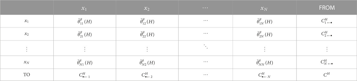
TABLE 1. Risk spillover matrix.

The element $C_{i\leftarrow •}^H$ in the “FROM” column of the connectedness matrix indicates risk spillover effects that country i receives from all other countries, that is, its total received spillover:

${\mathit{C}}_{\mathit{i}\leftarrow •}^{\mathit{H}}=\frac{{\displaystyle \sum }_{\begin{array}{c}\mathit{j}=\mathbf{1}\\ \mathit{j}\ne \mathit{i}\end{array}}^{\mathit{N}}{\stackrel{\sim }{\mathit{\theta }}}_{\mathit{i}\mathit{j}}^{\mathit{g}}\left(\mathit{H}\right)}{{\displaystyle \sum }_{\mathit{i},\mathit{j}=\mathbf{1}}^{\mathit{N}}{\stackrel{\sim }{\mathit{\theta }}}_{\mathit{i}\mathit{j}}^{\mathit{g}}\left(\mathit{H}\right)}=\frac{{\displaystyle \sum }_{\begin{array}{c}\mathit{j}=\mathbf{1}\\ \mathit{j}\ne \mathit{i}\end{array}}^{\mathit{N}}{\stackrel{\sim }{\mathit{\theta }}}_{\mathit{i}\mathit{j}}^{\mathit{g}}\left(\mathit{H}\right)}{\mathit{N}}(23)$

Similarly, the element $C_{•\leftarrow i}^H$ in the “TO” row of the connectedness matrix represents the risk contagion effects from country i to all other countries, that is, its total exported spillover:

${\mathit{C}}_{•\leftarrow \mathit{i}}^{\mathit{H}}=\frac{{\displaystyle \sum }_{\begin{array}{c}\mathit{j}=\mathbf{1}\\ \mathit{j}\ne \mathit{i}\end{array}}^{\mathit{N}}{\stackrel{\sim }{\mathit{\theta }}}_{\mathit{j}\mathit{i}}^{\mathit{g}}\left(\mathit{H}\right)}{{\displaystyle \sum }_{\mathit{i},\mathit{j}=\mathbf{1}}^{\mathit{N}}{\stackrel{\sim }{\mathit{\theta }}}_{\mathit{j}\mathit{i}}^{\mathit{g}}\left(\mathit{H}\right)}=\frac{{\displaystyle \sum }_{\begin{array}{c}\mathit{j}=\mathbf{1}\\ \mathit{j}\ne \mathit{i}\end{array}}^{\mathit{N}}{\stackrel{\sim }{\mathit{\theta }}}_{\mathit{j}\mathit{i}}^{\mathit{g}}\left(\mathit{H}\right)}{\mathit{N}}(24)$

Then the net spillover effect $C_i^H$ of country i to all other countries can be calculated as

${\mathit{C}}_{\mathit{i}}^{\mathit{H}}={\mathit{C}}_{•\leftarrow \mathit{i}}^{\mathit{H}}-{\mathit{C}}_{\mathit{i}\leftarrow •}^{\mathit{H}}(25)$

The total spillover effect $C^H$ by all countries is

${\mathit{C}}^{\mathit{H}}=\frac{{\displaystyle \sum }_{\begin{array}{c}\mathit{i},\mathit{j}=\mathbf{1}\\ \mathit{i}\ne \mathit{j}\end{array}}^{\mathit{N}}{\stackrel{\sim }{\mathit{\theta }}}_{\mathit{i}\mathit{j}}^{\mathit{g}}\left(\mathit{H}\right)}{{\displaystyle \sum }_{\mathit{i},\mathit{j}=\mathbf{1}}^{\mathit{N}}{\stackrel{\sim }{\mathit{\theta }}}_{\mathit{i}\mathit{j}}^{\mathit{g}}\left(\mathit{H}\right)}=\frac{{\displaystyle \sum }_{\begin{array}{c}\mathit{i},\mathit{j}=\mathbf{1}\\ \mathit{i}\ne \mathit{j}\end{array}}^{\mathit{N}}{\stackrel{\sim }{\mathit{\theta }}}_{\mathit{i}\mathit{j}}^{\mathit{g}}\left(\mathit{H}\right)}{\mathit{N}}(26)$

$C^H$ is equal to the sum of all elements in the “FROM” column or the “TO” row.

3 Empirical analysis

3.1 Data and descriptive statistics

The international crude oil futures market has long been dominated by two influential benchmarks, West Texas Intermediate (WTI) on the New York Mercantile Exchange (NYMEX) and Brent on the Intercontinental Exchange (ICE). Compared to Brent crude oil, WTI crude has lower impurities, higher utilization rate, and can be refined into more types of fuel oil. WTI futures have stronger liquidity and relative insensitivity to speculative bubbles (Ajmi et al., 2021; Zhang & Zhang, 2015). This paper selects the daily data of WTI crude oil futures prices and the closing of 28 major global stock market indexes from 7 January 2008 to 30 December 2020 as the sample. All data are retrieved from the Wind financial database. Please see the data sheet in Supplementary material for the dataset. The 28 countries include 11 non-signatories—China, India, Brazil, Israel, South Korea, Mexico, Indonesia, South Africa, Thailand, Turkey, and Malaysia, and 17 signatories—Australia, Austria, Belgium, Denmark, Finland, France, Germany, Greece, Italy, Japan, Netherlands, New Zealand, Norway, Spain, Sweden, Switzerland, and United Kingdom.¹ The first commitment period is from 7 January 2008 to 27 December 2012, and the second commitment period is from 7 January 2013 to 30 December 2020. In consideration of space, only the descriptive statistical results of the crude oil market and selected stock markets are reported in Table 2.

TABLE 2

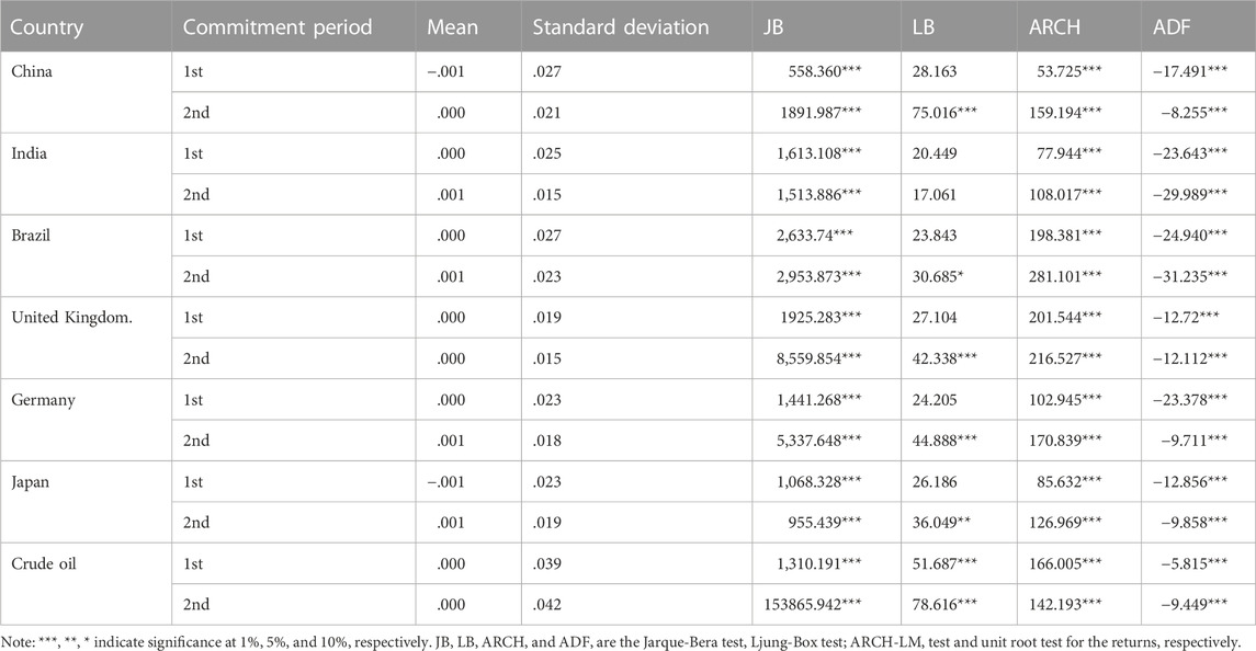
TABLE 2. Descriptive statistical results.

The standard deviations show that the volatility of most stock markets in the first commitment period is greater than that in the second commitment period, and the volatility of the crude oil market is much higher than that of the stock markets. The Jarque-Bera tests show that the return series do not follow the normal distribution during either commitment period. The LB and ARCH statistics indicate that most stock markets and the crude oil market exhibit autocorrelation and heteroscedasticity. The ADF statistics suggest that all return series are stationary.

3.2 Correlation and risk spillover

3.2.1 Estimation of marginal distributions

According to the principle of maximum log-likelihood estimation, the ARMA (1,1)-TGARCH(1,1) model is selected for the crude oil market and all stock markets to characterize their marginal distributions. The estimation results and fitting effects of the crude oil market and selected stock markets are reported in Supplementary Tables A1, A2 in Supplementary Appendix.

The ARCH coefficient $\alpha$ and the GARCH coefficient $\beta$ indicate that all stock markets and the crude oil market exhibit volatility and volatility clustering effects. The asymmetric effect parameter λ shows that during both commitment periods, the crude oil market and stock markets of Brazil, United Kingdom, Germany, and Japan demonstrate leverage effects and are susceptible to negative news because of their positive λ. The main reason for such phenomena is that most investors are risk averse. The emergence of adverse information affects investors’ investment decisions and trading behaviors, often causing them to sell in large quantity out of fear. LB, LB2, and ARCH statistics suggest that the standard residuals of most stock markets and the crude oil market have no autocorrelation or heteroscedasticity during the two commitment periods. KS and AD tests confirm that after the probability integral transformation, the marginal distributions all follow the uniform distribution.

3.2.2 Regime switching characteristics

To further analyze the return characteristics, this paper adopts the Markov regime switching model to examine the periodicity and asymmetry of the crude oil market and 28 stock markets. The estimation results are shown in Table 3. The transition probabilities indicate that both bear market and bull market have strong continuity, that is, the probabilities for a rising or falling state of the return to continue are almost all above .8. For example, the durations of bear and bull markets for the Chinese stock market are 7.519 and 17.857 days respectively. The bull market in China, India, United Kingdom, and Japan lasts longer than the bear market, while the bear market in the Brazilian and German stock markets as well as the crude oil market lasts longer than the bull market. The regime-switching behavior in stock and crude oil prices manifests financial market psychology and underlying capital movements. When institutional capital buys or sells stocks or crude oil futures according to a market’s expected prosperity, retail investors tend to follow due to the herding effect. Consequently, stock and crude oil prices often demonstrate a certain degree of trend within a short period of time.

TABLE 3

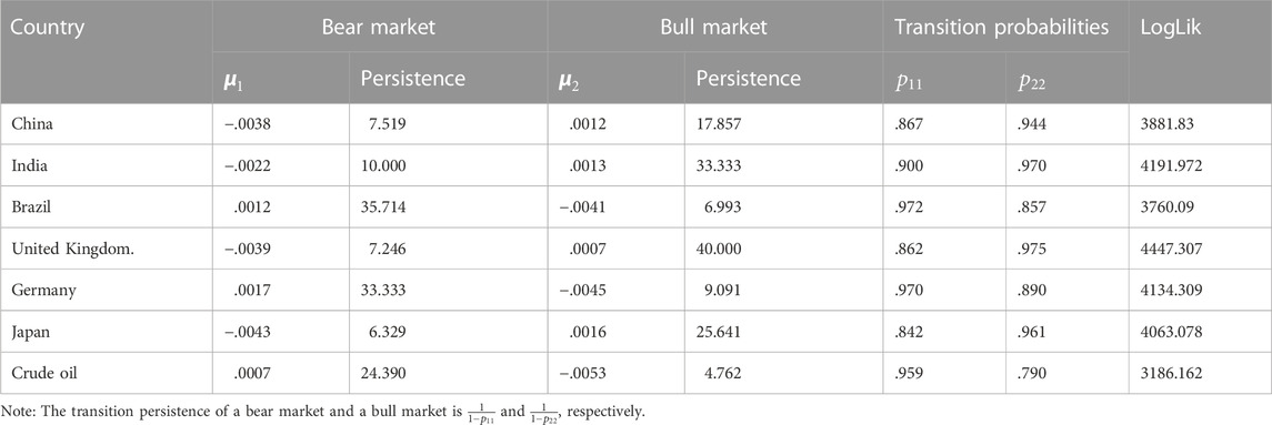
TABLE 3. Estimates for Markov regime switching model.

3.2.3 Correlation between crude oil and stock markets

Next, we use the TV Normal Copula function, the TV Student t Copula function, the TV SJC Copula function, the TV Plackett Copula function, the TV Clayton Copula function, and the TV Gumbel Copula function to connect the marginal distribution of the crude oil market and stock markets. The optimal Copula function is selected according to the AIC criterion. Table 4 shows the Copula parameter estimation results between the crude oil market and selected stock markets, where the TV Student t or SJC Copula function is the preferred model.

TABLE 4

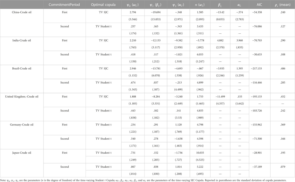
TABLE 4. Parameter estimates of copula functions.

The last column in Table 4 shows the mean value of Spearman’s rank correlation coefficient ${\rho }_s$. Along with Figure 1, they reveal the dynamic correlation between the crude oil market and global stock markets. There are positive correlations between global stock markets and the crude oil market, and the correlations are weaker during the second commitment period. The main reason is that corporations have developed and adopted more green technologies by the second commitment period, which somewhat reduce their degree of dependence on crude oil. As the stock markets serve as a “barometer” of corporations’ operations, the correlations become weaker in the second commitment period.

FIGURE 1

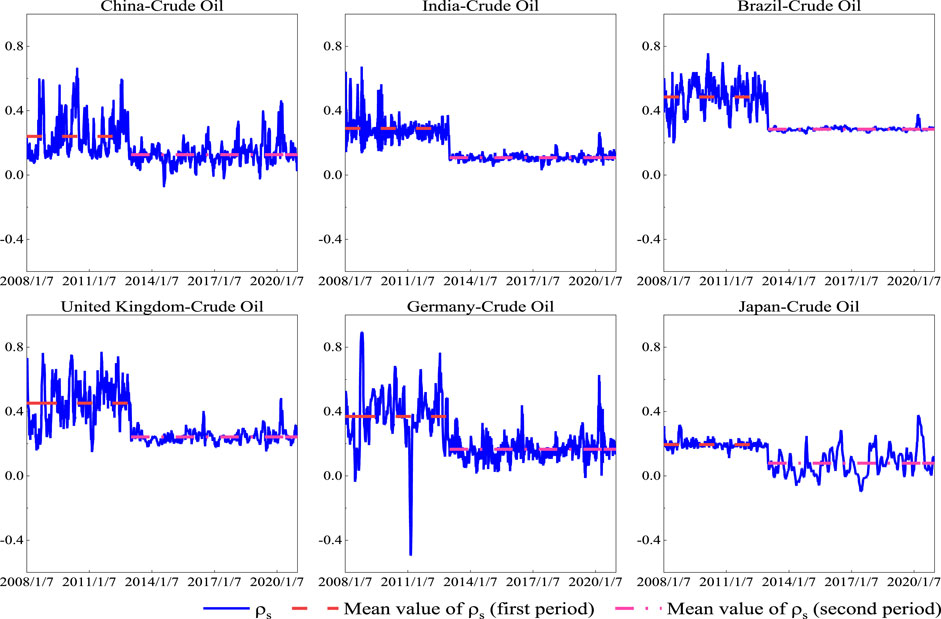
FIGURE 1. Spearman’s dynamic correlation (${\rho }_s$) between crude oil and stock markets.

3.2.4 Risk spillover effect between crude oil market and stock markets

Time-varying Copula-CoVaR models can not only measure the correlation between the crude oil and stock markets, but also gauge the risk spillover effect between the two.

$CoVa{R}_{\mathrm{0.05,0.05}}^{down}$ and $CoVa{R}_{\mathrm{0.05,0.05}}^{up}$ indicate the tail risk of stock markets ― from the perspective of long and short positions respectively ― conditional on crude oil market being at risk. The difference between $CoVa{R}_{\mathrm{0.05,0.05}}^{down}$ and $Va{R}_{0.05}^{down}$ characterizes the downside spillover effect, and the difference between $CoVa{R}_{\mathrm{0.05,0.05}}^{up}$ and $Va{R}_{0.05}^{up}$ depicts the upside spillover effect. The results are shown in Figure 2.

FIGURE 2

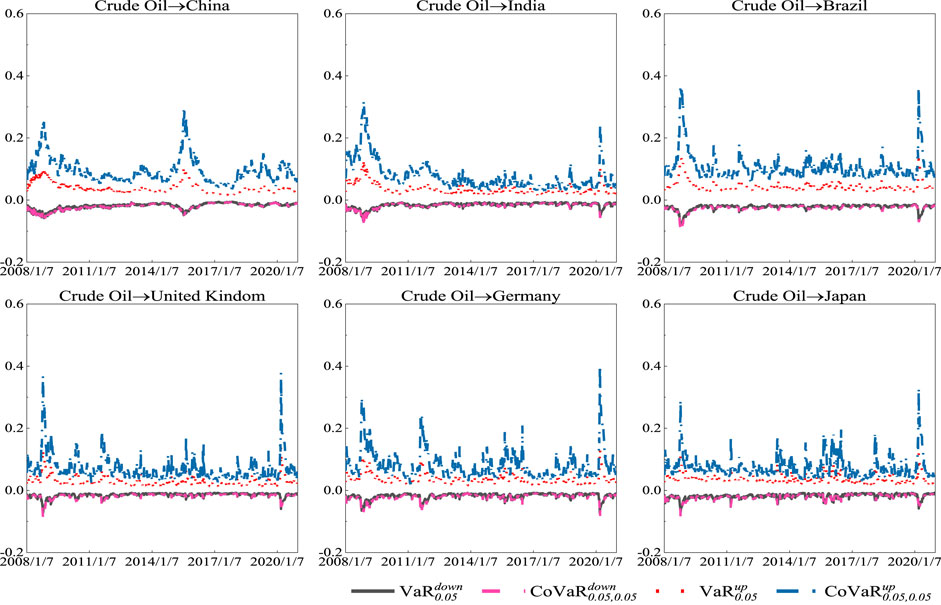
FIGURE 2. Tail risk and spillover effects between oil and stock markets.

It is evident in Figure 2 that in both commitment periods, the upside tail risk of the crude oil market to the stock markets in various countries is significantly higher than the downside tail risk. The upside tail risk has obvious spillover effects (as indicated by the discrepancy between $CoVa{R}_{\mathrm{0.05,0.05}}^{up}$; $Va{R}_{0.05}^{up}$), especially during and shortly after the 2008 global financial crisis, 2015 Chinese stock market crisis, and 2020 global pandemic. In contrast, downside tail risk spillover effects are much limited. The asymmetry in tail risk spillover demonstrates differences in the association between crude oil and stock markets under diverse market conditions. Global markets seem to be more susceptible to the impact of good news. Optimism in economic prosperity has a more notable impact on energy and the stock markets.

Table 5 shows through ${\Delta CoVaR}_{\mathrm{0.05,0.05}}^{down}$ and ${\Delta CoVaR}_{\mathrm{0.05,0.05}}^{up}$ the downside risk spillover effect and upside risk spillover effect of the crude oil market to the stock markets in 28 countries. The mean values of ${\Delta CoVaR}_{\mathrm{0.05,0.05}}^{down}$ and ${\Delta CoVaR}_{\mathrm{0.05,0.05}}^{up}$ for most countries in the second commitment period are smaller than those in the first commitment period. These results echo the weaker correlations in the second commitment period, during which more advanced green technologies had been developed, reducing countries’ reliance on crude oil. Therefore, the risk spillover by extreme crude oil market is reduced. In the meantime, during the two commitment periods, the crude oil market has both upside and downside risk spillover effects to most stock markets, but the upside risk spillover effects are much stronger than the downside spillover effects. This finding suggests that short positions in stock markets are more susceptible to risk spillover from the crude oil market than long positions.

TABLE 5

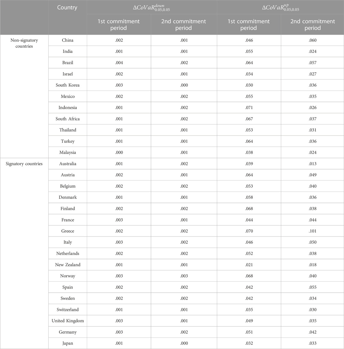
TABLE 5. Risk spillover effects indicated by $∆CoVa\mathrm{R.}$

3.3 Cross-country risk spillover network analysis

Based on the risk connectedness network proposed by Diebold and Yilmaz (2012, 2014), this section constructs a risk spillover index through the CoVaR of the crude oil market to the stock markets of various countries. An analysis of the topological characteristics of static and dynamic tail risk spillovers determines the risk exporters and risk receivers among signatories and non-signatories. A generalized variance decomposition based on the Adaptive Lasso-VAR model is established using CoVaR values, for which the optimal lag order is selected according to AIC. Following Diebold and Yilmaz (2012) and Liu et al. (2022), the forecast period H is set to 10 days (i.e., two trading weeks).

3.3.1 Static network analysis

First, the static network analysis is conducted to examine the risk spillover characteristics among the stock markets conditional on the crude oil market at risk during the two commitment periods, with the results shown in Table 6. Due to space limitations, only the top five and bottom five countries in each category—TO, FROM, and NET—are listed. Take the risk spillover characteristics of ${CoVaR}_{\mathrm{0.05,0.05}}^{down}$ during the first commitment period as an example. France, Netherlands, Germany, United Kingdom, and Sweden are the top five countries in terms of the net spillover value of ${CoVaR}_{\mathrm{0.05,0.05}}^{down}$ — which are all greater than zero—indicating that these five countries’ stock markets are the net exporters of risk spillovers in the first commitment period. In contrast, during the first commitment period, Thailand, New Zealand, Denmark, China, and Indonesia are ranked in the bottom five countries in terms of ${CoVaR}_{\mathrm{0.05,0.05}}^{down}$ net spillover value—which are all negative—indicating that the stock markets of these five countries are main receivers of risk spillover.² These results suggest that signatories are the primary risk exporter while non-signatories usually play the role of risk receivers. Most signatories have highly developed financial markets where capital and information flow more freely. Therefore, due to the influence of prevalent market sentiment and international investment strategy adjustments, the stock markets of signatories tend to transmit more risks to those of non-signatories.

TABLE 6

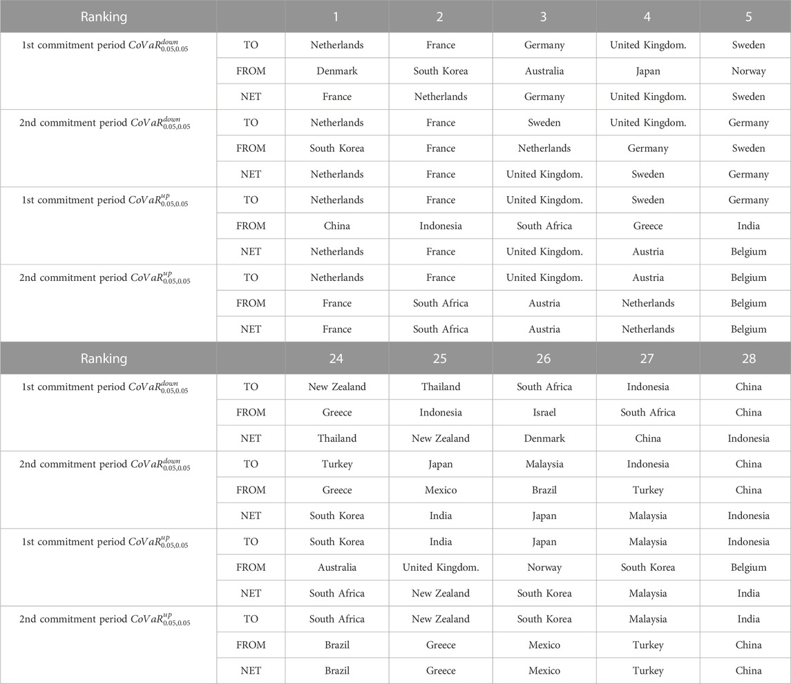
TABLE 6. Static risk spillover effects (top and bottom 5 countries).

3.3.2 Dynamic network analysis

The static network analysis above explores risk spillover between the stock markets of various countries when the crude oil market is at risk by estimating the models’ fixed parameters over a sample period. Since risk spillovers between stock markets are time-varying, this section draws on Diebold and Yilmaz (2012) to conduct dynamic spillover analysis with a step of 1 and a rolling window of 200. That is, the first spillover is calculated with the data from the 1st to the 200th sample observations, and the second spillover is calculated with the data from the 2nd to the 201st sample observations, and so on.

Figure 3 depicts the total tail risk spillovers — ${CoVaR}_{\mathrm{0.05,0.05}}^{down}$ or ${CoVaR}_{\mathrm{0.05,0.05}}^{up}$ — in the stock markets of the 28 countries when the crude oil market is at risk during the two commitment periods. It can be seen that during the first commitment period ${CoVaR}_{\mathrm{0.05,0.05}}^{down}$ and ${CoVaR}_{\mathrm{0.05,0.05}}^{up}$ in the stock markets fluctuate between 80% and 90%. Compared to the first commitment period, the fluctuation range in the second commitment period is wider, when ${CoVaR}_{\mathrm{0.05,0.05}}^{down}$ and ${CoVaR}_{\mathrm{0.05,0.05}}^{up}$ swing between 75% and 95%. In either commitment period, the risk spillovers from other countries account for more than 75% of total risk. This indicates that when the crude oil market is at risk, the tail risk of each stock market mainly comes from stock markets in other countries. Internally generated tail risk is relatively low.

FIGURE 3

FIGURE 3. Total spillovers. Note: The unit of the vertical axis is percentage.

Three marked periods in Figure 3 are worth close examinations. The first is the 2008 global financial crisis and its aftermath. Due to deep debt crisis and high deficit levels, panic was widespread in the market and the economy in many countries went into recession. The total tail risk spillover, ${CoVaR}_{\mathrm{0.05,0.05}}^{down}$ and ${CoVaR}_{\mathrm{0.05,0.05}}^{up}$, hovered close to 90%. The implementation of projects under the Kyoto Protocol was affected due to budget cuts and reduced spending. With the forceful actions taken by governments and international institutions such as IMF and EU, the risk spillover effect was subsequently contained, which is visible in the abrupt plummet in ${CoVaR}_{\mathrm{0.05,0.05}}^{down}$ and ${CoVaR}_{\mathrm{0.05,0.05}}^{up}$ in mid 2010. The second dramatic period is mid 2015. The total spillover effects of ${CoVaR}_{\mathrm{0.05,0.05}}^{down}$ and ${CoVaR}_{\mathrm{0.05,0.05}}^{up}$ rose sharply from June to August 2015, when the circuit breaker was triggered in the US stock market and thousands of stocks reached limit down repeatedly in the Chinese stock market. The third notable period is February to March 2020. With the outbreak of the global pandemic, many enterprises were forced to suspend or scale down production or business. The interruptions in capital flow and production chain greatly increased risk spillovers in global stock markets.

Since the total spillovers do not reflect the directional information of risk spillover, “TO all others” $C_{•\leftarrow i}^H$ and “FROM all others” $C_{i\leftarrow •}^H$ represent the risk spillover generated and received by country i respectively, which are shown in Supplementary Figure A1 through Supplementary Figure A4 in Supplementary Appendix. Supplementary Figures A1, A2 show the risk spillover by each country to the other 27 countries when the oil market is at risk during the two commitment periods. Overall, $C_{•\leftarrow i}^H$ of ${CoVaR}_{\mathrm{0.05,0.05}}^{down}$ and ${CoVaR}_{\mathrm{0.05,0.05}}^{up}$ follow similar trends for almost all countries. In both commitment periods, risk spillovers by non-signatories to others are generally below 4%. In contrast, risk spillovers of signatories are generally above 4%, suggesting that they yield greater risk spillover effects to others. Therefore, when the crude oil market is at risk, signatories possess stronger risk spillover effects to others than non-signatories. Supplementary Figures A3, A4 illustrate the risk spillover received by each country from the other 27 countries, $C_{i\leftarrow •}^H$, during the two commitment periods respectively. Except for China, the upside and downside risk spillover effects received by most countries are generally stable at around 3% across the two commitment periods. In contrast to Supplementary Figures A1, A2, signatories and non-signatories show little difference in risk spillover received in Supplementary Figures A3, A4.

Figures 4, 5 characterize the net risk spillover ($C_i^H$) by each country, which is defined as the difference between $C_{•\leftarrow i}^H$ and $C_{i\leftarrow •}^H$. A positive $C_i^H$ indicates that a country is an overall risk exporter, while a negative $C_i^H$ indicates an overall risk receiver. During both commitment periods, the net spillover values of ${CoVaR}_{\mathrm{0.05,0.05}}^{down}$ and ${CoVaR}_{\mathrm{0.05,0.05}}^{up}$ of non-signatories are mostly negative, indicating that they are net risk spillover receivers. In contrast, the net spillover values of ${CoVaR}_{\mathrm{0.05,0.05}}^{down}$ and ${CoVaR}_{\mathrm{0.05,0.05}}^{up}$ are mostly positive for signatories, suggesting they are net risk spillover exporters. The fundamental reason behind this contrast is that the signatories are all developed countries that occupy advantageous economic positions in the world. When their economies or stock market experience crisis or turbulence, other countries will quickly feel the impact via the global financial system. Therefore, the risk exported by signatories to other countries is usually higher than what they import.

FIGURE 4

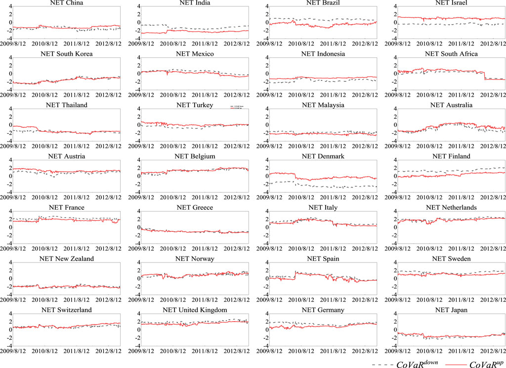
FIGURE 4. Net spillovers (1st commitment period). Note: The unit of the vertical axis is percentage.

FIGURE 5

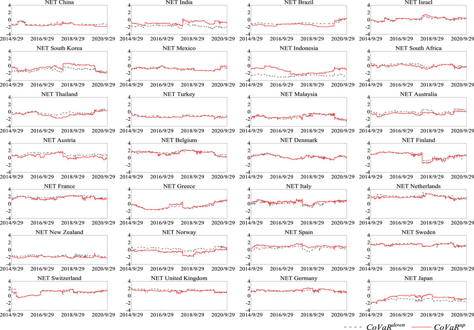
FIGURE 5. Net spillovers (2nd commitment period). Note: The unit of the vertical axis is percentage.

4 Conclusion

This paper examines and compares the correlation between the crude oil market and 28 major global stock markets and risk spillover effects during the first and second commitment periods of the Kyoto Protocol. Our major findings are as follows.

There are positive correlations between the crude oil market and stock markets in the world. In comparison, the correlations and risk spillovers between the crude oil and stock markets are weaker in the second commitment period. In addition, during both commitment periods, the crude oil market has risk spillover effects on most stock markets, and the upside risk spillover effect is stronger than the downside effect. This means that compared to long positions, short positions in stock markets are more susceptible to risk spillovers from the crude oil market. Last but not least, according to the total spillover, when the crude oil market is at risk, the tail risk of a stock market mainly comes from risk spillover of other countries rather than from within. The dynamic network analysis reveals that non-signatories are mostly net receivers of risk spillovers, while signatories are net exporters of risk spillovers when the crude oil market is at risk.

The findings in this study offer some advice to market participants and regulators. Stock market investors should be aware of the risk spillover effects from the crude oil market. When formulating and adjusting their portfolios, investors should assess the relationship between crude oil and stock markets to mitigate potential risk caused by extreme oil price fluctuations. As the upside spillover effect of the crude oil market on stock markets is much stronger than the downside effect, stock investors taking short positions should be particularly keen of risk spillover from extreme crude oil market. Overall, investors should maintain a prudent attitude and conduct rational analysis when making investment to avoid being overwhelmed by market sentiment or herding in financial markets. Financial regulators should be prepared for cross-market and cross-border risk contagion. Besides designing and implementing prudential policies to mitigate tail risks in individual markets, they should also pay attention to the risk spillover effects between different markets, and improve cross-market risk handling and regulatory coordination. In particular, since signatories usually export risk spillovers to non-signatories when the crude oil market is at risk, it would be worthwhile to discuss a financial firewall mechanism to prevent the outbreak and spread of financial crisis. Regular communications among regulators in different countries would facilitate international cooperation and coordination.

This study focuses on the relationship between global stock markets and the crude oil market. In reality, besides stock and crude oil markets, investors often also participate in foreign currencies, fixed income securities, and gold investment, thus benefiting from enhanced diversification or hedging. This paper uses the time-varying Copula-CoVaR model to study the correlation and risk spillover between stock and crude oil markets, but does not consider the impact of exchange rates, interest rates, gold, or other factors. The conventional multivariate Copula model requires that the correlation between each pair of variables is identical, which does not fit the reality of multi-market portfolios. As a future project, we plan to employ the vine Copula model to describe the complex interdependence among various financial markets. By calculating CoVaR, we can explore the risk spillover effects between the markets of crude oil, foreign currencies, fixed income securities, and gold, as well as stocks markets of various countries. Generalized variance decomposition based on the Adaptive Lasso-VAR model would enable the construction of a risk spillover network to identify risk exporters and receivers.

Data availability statement

The original contributions presented in the study are included in the article/Supplementary Material, further inquiries can be directed to the corresponding author.

Author contributions

JS contributes mainly to the conceptualization and the research design; JL is mainly responsible for model construction and implementation using programming software; JY is dedicated to validation and editing the article; YW and JL are responsible for drafting the paper and data analysis.

Funding

This research is supported by the National Natural Science Foundation of China (grant numbers: 71973056 and 71561011) and F.C. Manning Chair in Business Administration endowment fund (Acadia University).

Conflict of interest

The authors declare that the research was conducted in the absence of any commercial or financial relationships that could be construed as a potential conflict of interest.

Publisher’s note

All claims expressed in this article are solely those of the authors and do not necessarily represent those of their affiliated organizations, or those of the publisher, the editors and the reviewers. Any product that may be evaluated in this article, or claim that may be made by its manufacturer, is not guaranteed or endorsed by the publisher.

Supplementary material

The Supplementary Material for this article can be found online at: https://www.frontiersin.org/articles/10.3389/fenvs.2023.1103625/full#supplementary-material

Supplementary Figure A1 | Directional spillovers: TO all others (1st commitment period).

Supplementary Figure A2 | Directional spillovers: TO all others (2nd commitment period).

Supplementary Figure A3 | Directional spillovers: FROM all others (1st commitment period).

Supplementary Figure A4 | Directional spillovers: FROM all others (2nd commitment period).

Supplementary Table A1 | Estimates of marginal distribution models (1st commitment period).

Supplementary Table A2 | Estimates of marginal distribution models (2nd commitment period).

Supplementary Table A3 | Directional risk spillovers based on static network.

SUPPLEMENTARY Data Sheet 1 | Closing prices of oil and stock markets.

Footnotes

¹Since the United States and Canada withdrew from the Kyoto Protocol, they are not included in the study.

²See the Supplementary Table A3 in Supplementary Appendix for the complete information of static risk spillovers for all sample countries.

References

Adrian, T., and Brunnermeier, M. K. (2016). CoVaR. Am. Econ. Rev. 106 (7), 1705–1741.doi:10.1257/aer.20120555

CrossRef Full Text

Ajmi, A. N., Hammoudeh, S., and Mokni, K. (2021). Detection of bubbles in WTI, brent, and dubai oil prices: A novel double recursive algorithm. Resour. Policy 70, 101956. doi:10.1016/j.resourpol.2020.101956

CrossRef Full Text | Google Scholar

Alamgir, F., and Amin, S. B. (2021). The nexus between oil price and stock market: Evidence from South Asia. Energy Rep. 7, 693–703. doi:10.1016/j.egyr.2021.01.027

CrossRef Full Text | Google Scholar

Arampatzidis, I., Dergiades, T., Kaufmann, R. K., and Panagiotidis, T. (2021). Oil and the U.S. stock market: Implications for low carbon policies. Energy Econ. 103, 105588. doi:10.1016/j.eneco.2021.105588

CrossRef Full Text | Google Scholar

Balcilar, M., Ozdemir, H., and Agan, B. (2022). Effects of COVID-19 on cryptocurrency and emerging market connectedness: Empirical evidence from quantile, frequency, and lasso networks. Phys. A Stat. Mech. its Appl. 604, 127885. doi:10.1016/j.physa.2022.127885

CrossRef Full Text | Google Scholar

Demirer, M., Diebold, F. X., Liu, L., and Yilmaz, K. (2018). Estimating global bank network connectedness. J. Appl. Econ. 33 (1), 1–15. doi:10.1002/jae.2585

CrossRef Full Text | Google Scholar

Depledge, J. (2022). The “top-down” Kyoto Protocol? Exploring caricature and misrepresentation in literature on global climate change governance. Int. Environ. Agreements Polit. Law Econ. 22, 673–692. doi:10.1007/s10784-022-09580-9

CrossRef Full Text | Google Scholar

Diebold, F. X., and Yilmaz, K. (2012). Better to give than to receive: Predictive directional measurement of volatility spillovers. Int. J. Forecast. 28 (1), 57–66. doi:10.1016/j.ijforecast.2011.02.006

CrossRef Full Text | Google Scholar

Diebold, F. X., and Yilmaz, K. (2014). On the network topology of variance decompositions: Measuring the connectedness of financial firms. J. Econ. 182 (1), 119–134. doi:10.1016/j.jeconom.2014.04.012

CrossRef Full Text | Google Scholar

Dogan, E., Chishti, M. Z., Alavijeh, N. K., and Tzeremes, P. (2022). The roles of technology and Kyoto Protocol in energy transition towards COP26 targets: Evidence from the novel GMM-PVAR approach for G-7 countries. Technol. Forecast. Soc. Change 181, 121756. doi:10.1016/j.techfore.2022.121756

CrossRef Full Text | Google Scholar

Giot, P., and Laurent, S. (2003). Value-at-Risk for long and short trading positions. J. Appl. Econ. 18 (6), 641–663. doi:10.1002/jae.710

CrossRef Full Text | Google Scholar

Hansen, B. E. (1994). Autoregressive conditional density estimation. Int. Econ. Rev. 35 (3), 705–730. doi:10.2307/2527081

CrossRef Full Text | Google Scholar

Huang, S., An, H., Huang, X., and Jia, X. (2018). Co-movement of coherence between oil prices and the stock market from the joint time-frequency perspective. Appl. Energy 221, 122–130. doi:10.1016/j.apenergy.2018.03.172

CrossRef Full Text | Google Scholar

Jamil, K., Liu, D., Gul, R. F., Hussain, Z., Mohsin, M., Qin, G., et al. (2022). Do remittance and renewable energy affect CO₂ emissions? An empirical evidence from selected G-20 countries. Energy and Environ. 33 (5), 916–932. doi:10.1177/0958305X211029636

CrossRef Full Text | Google Scholar

Ji, Q., Liu, B.-Y., Zhao, W.-L., and Fan, Y. (2020). Modelling dynamic dependence and risk spillover between all oil price shocks and stock market returns in the BRICS. Int. Rev. Financial Analysis 68, 101238. doi:10.1016/j.irfa.2018.08.002

CrossRef Full Text | Google Scholar

Jiang, Y., Wang, G.-J., Ma, C., and Yang, X. (2021). Do credit conditions matter for the impact of oil price shocks on stock returns? Evidence from a structural threshold VAR model. Int. Rev. Econ. Finance 72, 1–15. doi:10.1016/j.iref.2020.10.019

CrossRef Full Text | Google Scholar

Kang, S. H., McIver, R., and Yoon, S.-M. (2017). Dynamic spillover effects among crude oil, precious metal, and agricultural commodity futures markets. Energy Econ. 62, 19–32. doi:10.1016/j.eneco.2016.12.011

CrossRef Full Text | Google Scholar

Khan, F. U., Rafique, A., Ullah, E., and Khan, F. (2022). Revisiting the relationship between remittances and CO2 emissions by applying a novel dynamic simulated ARDL: Empirical evidence from G-20 economies. Environ. Sci. Pollut. Res. 29 (47), 71190–71207. doi:10.1007/s11356-022-20768-z

CrossRef Full Text | Google Scholar

Kilian, L., and Park, C. (2009). The impact of oil price shocks on the U.S. stock market. Int. Econ. Rev. 50 (4), 1267–1287. doi:10.1111/j.1468-2354.2009.00568.x

CrossRef Full Text | Google Scholar

Kuriyama, A., and Abe, N. (2018). Ex-post assessment of the Kyoto Protocol-quantification of CO2 mitigation impact in both Annex B and non-Annex B countries. Appl. Energy 220, 286–295. doi:10.1016/j.apenergy.2018.03.025

CrossRef Full Text | Google Scholar

Liu, B.-Y., Fan, Y., Ji, Q., and Hussain, N. (2022). High-dimensional CoVaR network connectedness for measuring conditional financial contagion and risk spillovers from oil markets to the G20 stock system. Energy Econ. 105, 105749. doi:10.1016/j.eneco.2021.105749

CrossRef Full Text | Google Scholar

Liu, S. Y., Fang, W., Gao, X. Y., Wang, Z., An, F., and Wen, S. B. (2020). Self-similar behaviors in the crude oil market. Energy 211, 118682. doi:10.1016/j.energy.2020.118682

CrossRef Full Text | Google Scholar

Ma, Z. F. (2012). The effectiveness of Kyoto Protocol and the legal institution for international technology transfer. J. Technol. Transf. 37 (1), 75–97. doi:10.1007/s10961-010-9190-7

CrossRef Full Text | Google Scholar

Maamoun, N. (2019). The Kyoto protocol: Empirical evidence of a hidden success. J. Environ. Econ. Manag. 95, 227–256. doi:10.1016/j.jeem.2019.04.001

CrossRef Full Text | Google Scholar

Madaleno, M., and Moutinho, V. (2017). A new LDMI decomposition approach to explain emission development in the EU: Individual and set contribution. Environ. Sci. Pollut. Res. 24 (11), 10234–10257. doi:10.1007/s11356-017-8547-y

PubMed Abstract | CrossRef Full Text | Google Scholar

Maghyereh, A., and Abdoh, H. (2022). Extreme dependence between structural oil shocks and stock markets in GCC countries. Resour. Policy 76, 102626. doi:10.1016/j.resourpol.2022.102626

CrossRef Full Text | Google Scholar

Mensi, W., Hammoudeh, S., Shahzad, S. J. H., and Shahbaz, M. (2017). Modeling systemic risk and dependence structure between oil and stock markets using a variational mode decomposition-based copula method. J. Bank. Finance 75, 258–279. doi:10.1016/j.jbankfin.2016.11.017

CrossRef Full Text | Google Scholar

Mohammed, S. D. (2020). Clean development mechanism and carbon emissions in Nigeria. Sustain. Account. Manag. Policy J. 11 (3), 523–551. doi:10.1108/Sampj-05-2017-0041

CrossRef Full Text | Google Scholar

Nicholson, W. B., Matteson, D. S., and Bien, J. (2015). VARX-L: Structured regularization for large vector autoregressions with exogenous variables. Int. J. Forecast. 33 (3), 627–651. doi:10.1016/j.ijforecast.2017.01.003

CrossRef Full Text | Google Scholar

Ramos, S. B., and Veiga, H. (2013). Oil price asymmetric effects: Answering the puzzle in international stock markets. Energy Econ. 38, 136–145. doi:10.1016/j.eneco.2013.03.011

CrossRef Full Text | Google Scholar

Raza, N., Shahzad, S. J. H., Tiwari, A. K., and Shahbaz, M. (2016). Asymmetric impact of gold, oil prices and their volatilities on stock prices of emerging markets. Resour. Policy 49, 290–301. doi:10.1016/j.resourpol.2016.06.011

CrossRef Full Text | Google Scholar

Reboredo, J. C., and Ugolini, A. (2016). Quantile dependence of oil price movements and stock returns. Energy Econ. 54, 33–49. doi:10.1016/j.eneco.2015.11.015

CrossRef Full Text | Google Scholar

Ren, Y., and Zhang, X. (2013). Model selection for vector autoregressive processes via adaptive Lasso. Commun. Statistics - Theory Methods 42 (13), 2423–2436. doi:10.1080/03610926.2011.611317

CrossRef Full Text | Google Scholar

Ren, Y., and Zhang, X. (2010). Subset selection for vector autoregressive processes via adaptive Lasso. Statistics Probab. Lett. 80 (23-24), 1705–1712. doi:10.1016/j.spl.2010.07.013

CrossRef Full Text | Google Scholar

Tran, T. M. (2022). International environmental agreement and trade in environmental goods: The case of Kyoto Protocol. Environ. Resour. Econ. 83, 341–379. doi:10.1007/s10640-021-00625-2

CrossRef Full Text | Google Scholar

Wang, G.-J., Xie, C., He, K., and Stanley, H. E. (2017). Extreme risk spillover network: Application to financial institutions. Quant. Finance 17 (9), 1417–1433. doi:10.1080/14697688.2016.1272762

CrossRef Full Text | Google Scholar

Wang, Z., Gao, X., Huang, S., Sun, Q., Chen, Z., Tang, R., et al. (2022). Measuring systemic risk contribution of global stock markets: A dynamic tail risk network approach. Int. Rev. Financial Analysis 84, 102361. doi:10.1016/j.irfa.2022.102361

CrossRef Full Text | Google Scholar

Wen, D., Wang, G.-J., Ma, C., and Wang, Y. (2019). Risk spillovers between oil and stock markets: A VAR for VaR analysis. Energy Econ. 80, 524–535. doi:10.1016/j.eneco.2019.02.005

CrossRef Full Text | Google Scholar

Xu, W., Ma, F., Chen, W., and Zhang, B. (2019). Asymmetric volatility spillovers between oil and stock markets: Evidence from China and the United States. Energy Econ. 80, 310–320. doi:10.1016/j.eneco.2019.01.014

CrossRef Full Text | Google Scholar

Zhang, C., and Chen, X. (2011). The impact of global oil price shocks on China's stock returns: Evidence from the ARJI(-h_t)-EGARCH model. Energy 36 (11), 6627–6633. doi:10.1016/j.energy.2011.08.052

CrossRef Full Text | Google Scholar

Zhang, Y.-J., and Ma, S.-J. (2019). How to effectively estimate the time-varying risk spillover between crude oil and stock markets? Evidence from the expectile perspective. Energy Econ. 84, 104562. doi:10.1016/j.eneco.2019.104562

CrossRef Full Text | Google Scholar

Zhang, Y.-J., and Zhang, L. (2015). Interpreting the crude oil price movements: Evidence from the Markov regime switching model. Appl. Energy 143, 96–109. doi:10.1016/j.apenergy.2015.01.005

CrossRef Full Text | Google Scholar

Zou, H. (2006). The adaptive Lasso and its oracle properties. J. Am. Stat. Assoc. 101 (476), 1418–1429. doi:10.1198/016214506000000735

CrossRef Full Text | Google Scholar