 Tino Fauk
 Petra Schneider
- Department Water, Environment, Civil Engineering and Safety, Magdeburg-Stendal University of Applied Sciences, Magdeburg, Germany
Motivation: Planting urban trees is important for urban development. Foliage reflects, scatters, and absorbs incoming shortwave solar radiation, thus reducing the energy flow to the underlying surface, including streets, houses, and humans. Shaded areas, with primarily anthropogenic substrates, are not as heated as nonshaded areas. Subsequently, temperature, radiation and its influence on morbidity of fauna and flora are comparatively lower in these areas.
Materials and Methods: Statistical methods were applied to assess the allometric functions of urban trees. The analyzed data were obtained from the tree cadaster of Magdeburg City, Germany, which contains information from 1936 to 2021. As of June 2022, the tree cadaster contained 89,766 trees. The tree species Acer campestre, Acer platanoides, Malus spp., and Quercus robur were subjected to investigation. Nine temperature optimum (TO)/precipitation optimum (PO) scenarios were considered, and their effects on the allometric relationships on the tree species were determined, respectively: 1. TO 17–19°C/PO 450–550 mm, 2. TO 19–21°C/PO 450–550 mm, 3. TO 21–23°C/PO 450–550 mm., 4. TO 17–19°C/PO 550–650 mm, 5. TO 19–21°C/PO 550–650 mm, 6. TO 21–23°C/PO 550–650 mm, 7. TO 17–19°C/PO 650–750 mm, 8. TO 19–21°C/PO 650–750 mm, 9. TO 21–23°C/PO 650–750 mm.
Results and Discussion: In six of nine scenarios, a significant correlation was evident for temperature. Water uptake was found to be significant in scenario 6. No significant correlation for competition and breast head diameter growth could be determined in any scenario. Five of the nine scenarios were significantly comparable. While competition was evident as conditionally non-significant (p-value = 0.069 & 0.058), for the elevation forecast in scenarios 3 & 6 only, dependence was evident in all other scenarios. Regarding the crown diameter, temperature was significant in 3 of 9 scenarios. No significant relationship was found for water uptake and competition.
Conclusions: No clear abiotic optimum could be identified. Thus, a continuous adjustment of the parameters is necessary to refine the growth functions. Moreover, the growth function adaptation according to the different age phases of trees might be considered on the long term.
1 Introduction
Planting urban trees is substantially important for the future development of urban spaces. The foliage reflects, scatters, and absorbs incoming shortwave solar radiation, thus reducing the energy flow to the underlying surface, including streets, houses, and humans (Mehra, 2021). Shaded areas, with primarily anthropogenic substrates, are not as heated as non-shaded areas; subsequently, the temperature radiation and its influence on morbidity are comparatively lower in shaded areas. An increase of even 1°C in the perceived temperature in summer causes a 3.12% increase in mortality (95% CI: 0.60%–5.72%) (Jahn, et al., 2013). Shortwave solar radiation is one influencing effect on the urban environment. Energy-rich wavelengths between 400 and 900 nm (visible light) can be manipulated with high tree density. The reduction of these wavelength in an oak wood for the temperate zone at 1 pm in spring and summer was 0% or 55–88% for the upper crown space (light crown), 10–25% or 95–98% for the lower crown space (shade crown), 20–55% or 97.5–99.25% for the shrub layer, and 20–55% or 98.5–99.5% for the herb layer as well (Kalusche, 2016). In addition to shading, which reduces direct solar radiation, plant transpiration can also have a cooling effect (Bongardt, 2006; Kuttler, 2010b; Moser, et al., 2017).
Plant species play an essential role in urban biodiversity and water balance. Necessary regulations (e.g., pest control by birds and bats and pollination by flies, beetles, bees, and butterflies) require balanced biodiversity, in which species sometimes depend on urban trees as a habitat. Urban trees have diverse ecological niches. Therefore, the importance of urban biodiversity cannot be overestimated (Gloor & Göldi Hofbauer, 2018).
In addition to providing biomass for district heating supply, the output of urban trees includes food and medical products. The flowers of Tilia cordata and T. platyphyllos have a wide range of medicinal applications and are considered medicinal plant components for gastritis (Riffel, 2021). Plant components of Crataegus monogyna and C. laevigata are used as treatments for the cardiovascular system (Riffel, 2021). Additionally, food production from fruit trees is an essential factor for sustainable food security.
The filtering functions of green areas have often been investigated and described (Baldacchini, et al., 2019; Wróblewska & Jeong, 2021). An Acer platanoides has a height of 9 m, a total leaf count of 41,000, an average leaf area of 68 cm2, a total leaf area of 278 m2, and a total dust layer of 2 kg during the growing season (of which 20% is particulate matter), while 3.5 kg of particulate matter is released into the environment during the same period (Breuste, et al., 2016).
Although landscape structures and associated biodiversity can promote human well-being (Kardan, et al., 2015; Moser, et al., 2017; Heise & Hallermayr, 2022), they also cause disadvantages (Bergmann & Straff, 2015; Moser, et al., 2017; Breuste, 2022). Trees, in particular, are essential for emotional sensation, as they can accompany people from childhood (e.g., apple trees in the garden) (Gebhard, 2020). A tree evokes positive emotions in humans, particularly through an intact, large crown with rich greenery (Heise & Hallermayr, 2022). Street trees have a predominantly positive emotional effect on people and can reduce stress (Flade, 2018). This stress reduction or recovery effect reduces susceptibility to accidents during road transport (Flade, 2018). In addition to the cultural and regulatory services that urban trees provide to ecosystems, they also provide services related to the allometric conditions of the individual tree species. Accordingly, functions for biomass, age determination, height growth, diameter growth, and trunk and crown shape have been created in different parts of the world (cf. Snorrason & Einarsson, 2006; Lukaszkiewicz & Kosmala, 2008; McPherson, et al., 2016; Hayat, et al., 2017; Moser, et al., 2017; Riedel, et al., 2017; Riedel & Kändler, 2017; Lei, et al., 2018; Lockow, 2022). Knowledge regarding primary growth conditions is crucial to determine the impact of tree species on human wellbeing. For example, the contribution of trees to urban ecosystem services often depends on tree dimensions. The ecosystem services of urban green infrastructure must be integrated into the general urban planning structure to ensure the sustainable development of urban spaces.
This study focuses on the basic theory for modeling the growth of breast height diameter (bhd), height, and crown diameter as a basis for estimating the ecosystem services of trees in cities as part of urban green infrastructure for municipal databases. The study area was the city of Magdeburg in Saxony-Anhalt, Germany. This study focused on identifying the factors that influence different allometric parameters. In the future, the performance of tree species in various urban ecosystems will be integrated into municipal planning tools.
2 Database and study area
Magdeburg, located in the heart of Germany, has a continental climate. This area is part of the Central German Dry Zone. The regional climate data were obtained from the Climate Data Center of the German Weather Service for weather station number 3126 (Magdeburg) [https://opendata.dwd.de/]. The folder contains the recorded values, explanations of the measurement technology used, and the identification of incorrect values. Temperature was defined as the daily average, maximum, and minimum at 2 m height. Temperature recordings were available for the period from 1 January 1881 to 31 December 2021. During this period, 731 records are missing, two of which were outside the time series under consideration, 30 between 1 and 31 April 1940. The remaining 699 missing values were recorded between 1 February 1945 and 31 December 1946 (WWII). Precipitation data were also used as influencing variables. Precipitation data were available for the period between 1 January 1881 and 31 December 2021. A total of 715 missing data records were observed, 14 of which were outside the observation period. Most shortfalls (700) were observed between 31 January 1945 and 31 December 1946. The last abiotic influencing variable, which was derived from the climate data, is the irradiation intensity. Sunshine duration, as a representative quantity, was recorded only from 1 October 1934. The years between 1934 and 31 December 1935 are marked by frequent data gaps. A total of 412 missing data values are recorded for the period before 1936. In March 1941, there were six data gaps. The period between 1 February 1945 and 31 March 1951 was characterized by total failure (2,250 values). The climate data gaps were filled through estimations based on the expected value.
The mean groundwater levels were obtained from the data on the Water Resources Services of the State Office for Flood Protection and Water Management (LHW) [https://gld.lhw-sachsen-anhalt.de/]. The groundwater gauges provide data for a time series of regular measurements between early 1960 and 2022. The mean groundwater level was represented as cm below ground level.
The infiltration coefficients were derived from the database for the soil property maps of the state of Saxony-Anhalt (©State Office for Geology and Mining Saxony-Anhalt) [available at: https://metaver.de/trefferanzeige?docuuid=C3444D0C-5AD7-4312-8A77-DB9B746940E3].
Range diagnoses were used to determine the relationship between individual growth rates. Plant-specific range diagnoses according to Jäger (2017) and Müller et al. (2021) were interpreted as described in Thomas (2018). For the temperature gradient, the flora zones and elevation stages were used. The elevation levels were interpreted according to Breckle and Rafiqpoor (2019) and Thomas (2018). Accordingly, it was observed a temperature decrease of 0.55 K and a precipitation increase of 100 mm per 100 m elevation increase.
The Magdeburg tree cadaster was used to derive the allometric basis to estimate the ecosystem services of tree species. As of June 2022, the tree cadaster Magdeburg included 89,766 individual trees. The tree species and genera Acer campestre, A. platanoides, Malus spp., and Quercus robur were used in this investigation. The tree cadaster contains position information, planting years, and information on the most crucial tree parameters, including bhd (or trunk circumference), height, and crown diameter. The tree species under investigation comprise about 23.2% (20,712 trees) of the total number of urban trees in Magdeburg on public green spaces that are registered in the tree cadaster. Of these 20,712 trees, 3,892 could be used to derive the allometric function. Most had no age information, which is why no corresponding correlations could be identified.
Acer campestre is widespread in Europe, tolerant of environmental stress, and prefers warm, sunny, nutrient-rich, and calcareous locations (StMELF, 2022b). According to Gloor and Göldi Hofbauer (2018), the biodiversity index (BD-I) is 4.0. As a field shrub, it is wind-tolerant and has an extensive cardiac root system (StMELF, 2022b). The ecological amplitude holds the average temperature and the precipitation for the geographical distribution. A. cam is located according to the plant geography continental stages (PGCS) between C1 and C6 for the European continent (Jäger, 2017). The annual mean temperature amplitude of this PGCS ranged between 0°C and 20°C, according to the mean annual temperature for Europe between 1991 and 2010. The precipitation in that area lies between 300 and 1800 mm per year, with a main distribution of <1,300 mm precipitation per year. According to Ellenberger, the plant-specific indicator value for the light number was five (for young trees), the temperature number was six, and the humidity number (soil) was five (Jäger, 2017). The yellow-to-orange autumn-colored leaves contrast with the often-gray urban infrastructure. Depending on its location and growth habit, A. campestre can reach standard heights of 1–5 m as a shrub and up to 20 m as a solitary tree (Jäger, 2017). The flowers are greenish-yellow and inconspicuous. Pollination during the flowering period from May to June is performed by wind and insects (Jäger, 2017). Its seeds are short-lived cold germs spread by the wind (Jäger, 2017). A total of 1,041 A. campestre were identified for further investigation.
Acer platanoides is a penumbra tree species but also tolerates full sun (StMELF, 2022c). The easily decomposable organic litter (StMELF, 2022c) can be used extensively in parks for humus buildup. According to Gloor and Göldi Hofbauer (2018), the BD-I is ∼3.6. Its yellowish-green flowers serve as a food source for insects from April to May. Its average height is 25 m, and it can be found as forest and street trees in Germany (Jäger, 2017). It is robust against industrial stress and is often used in public greenery (StMELF, 2022c). It has a deep, compact root system that can reach lower soil layers (Georg August University Göttingen, Germany, n.d). The PGCS is between C2 and C5 for the European continent (Jäger, 2017). The mean annual temperature ranges from 0°C to 15°C, and the annual precipitation ranges from 600 to a regional maximum of 1800 mm. It can also be used to produce furniture (StMELF, 2022c). A total of 1,140 A. platanoides specimens were included in this study.
Malus spp. belong to the rose family (Rosaceae), which is diverse due to human selection, the feralization of cultivated forms, and bastard formation (StMELF, 2022a). Due to its floral splendor, it is a vital insect food plant. In addition, fruits serve as a food source. According to Gloor and Göldi Hofbauer (2018), the BD-I was 4.2. Malus spp. and are 2–10 m high, depending on the species. The flowering period is from April to May (Jäger, 2017). It is a shallow rooter often used in landscapes as hedges and for mixed planting (StMELF, 2022a). The PGCS for Malus domistica is between C5–C7 for the west Asian continent; otherwise, Malus sylvestris ranges from C1 to C7. The annual precipitation for that area lies between 300–1800 mm per year. A total of 540 M. spp. exemplars were used in this study.
Quercus robur is widespread in Germany (StMELF, 2022d) but has a decreasing trend (Jäger, 2017). Q. robur tolerates waterlogging but not groundwater stress (StMELF, 2022d). Trees represent diverse ecological niches and are valuable for biodiversity. The BD-I is 5.0 out of the 5.0 possible scale points (Gloor & Göldi Hofbauer, 2018). Q. robur has a deep taproot and (StMELF, 2022d) grows to a height of 40 m (Jäger, 2017). Q. robur blooms in May. A total of 1,171 individual Quercus robur trees were considered in this study.
3 Methods
First, the factors influencing the allometric conditions were examined. Multiple regression identified an essential relationship between the immediate environment, climate conditions, and specific growth. The main model concept for the simulation of urban climate conditions and the coupled process with the urban green infrastructure is shown in the following Figure 1.
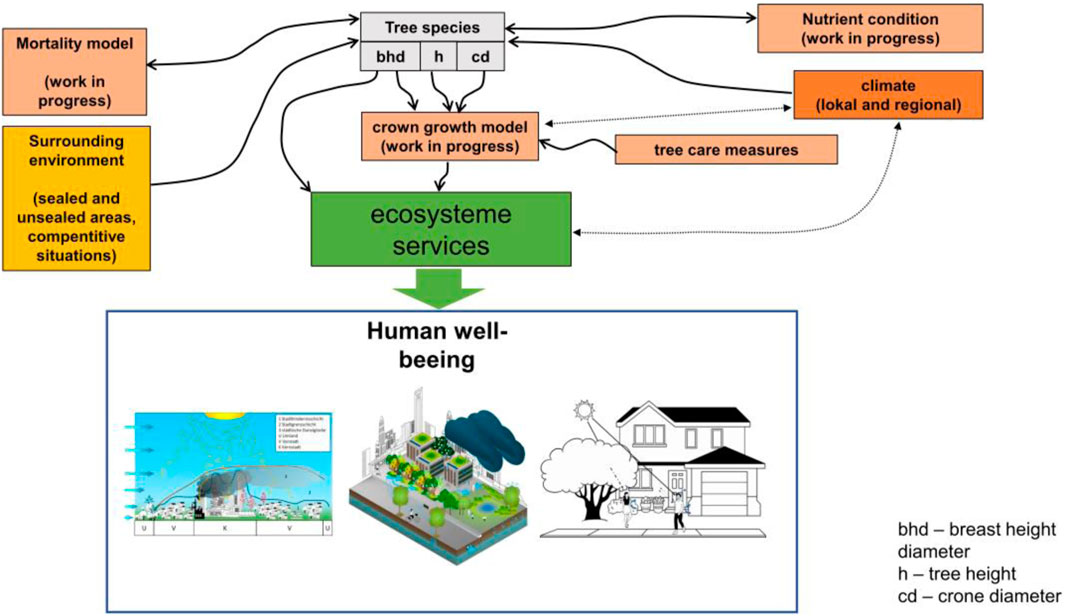
FIGURE 1. Principle of the model of urban trees for urban planning.
According to our null hypothesis, climatic conditions and the surrounding environment do not influence the allometric growth conditions (Equation 34). Therefore, the null hypothesis can be discarded if an effect is registered in the multiple regression analysis.
Environmental effects should be examined for species-specific ecological amplitude. For this purpose, maximum daily values of 17°C–19°C, 19°C–21°C, and 21°C–23°C and annual optimum precipitation ranges of 450 mm–550 mm, 550 mm–650 mm, and 650 mm–750 mm were investigated as the optimal temperature conditions. The combinations of the respective amplitude resulted in nine scenarios. In scenarios 1–3, the annual precipitation (optimum) was 450 mm–550 mm with changing temperature optima from 17°C–19°C and 21°C–23°C. Scenarios 4–6 investigated an annual precipitation optimum between 550 mm–650 mm with the likewise changing temperature optima as scenarios 1–3. In scenarios 7–9, the optimum annual precipitation was set as an ecological amplitude between 650 mm–750 mm, and all temperature optima were considered.
The following multiple regression model was used to identify the influencing factors. Breast height diameter (
The mean error of the expected value was determined as follows:
For further processing, a normally distributed random variable was used for the periods concerned and the expected climatic conditions. To do so, the 95% confidence interval was interpreted as follows:
The final estimate was made in the interval:
Figure 2 should be consulted for a first impression of the data completion. In the following, the daily maximum temperature was used to derive the energy production and the lower activity during physiological stress. Photosynthesis as an energy supplier for the tree is dependent on the ambient temperature and solar radiation. If this ambient temperature is outside a plant-specific temperature level
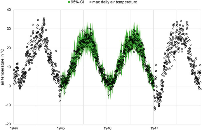
FIGURE 2. Example of the maximum daily temperature curve in the growing season in 1944 and 1947 from data recording and 1945 and 1946 with estimated data points and 95% confidence intervals.
Figure 3 shows the ranges of the examined relative plant-physiological optima. Next, the daily
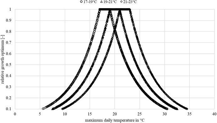
FIGURE 3. Sample illustration of the relative growth optimum
The absolute daily ratings were related to the number of vegetation periods experienced at the theoretical optimum. The researched tree species were in zonobiome VI. The vegetation period was interpreted as the moving average (
where
The growing season for the year j was calculated as follows:
Figure 4 shows the calculated growing season. The summed days of the growing season since the tree was planted were calculated using the following equation:
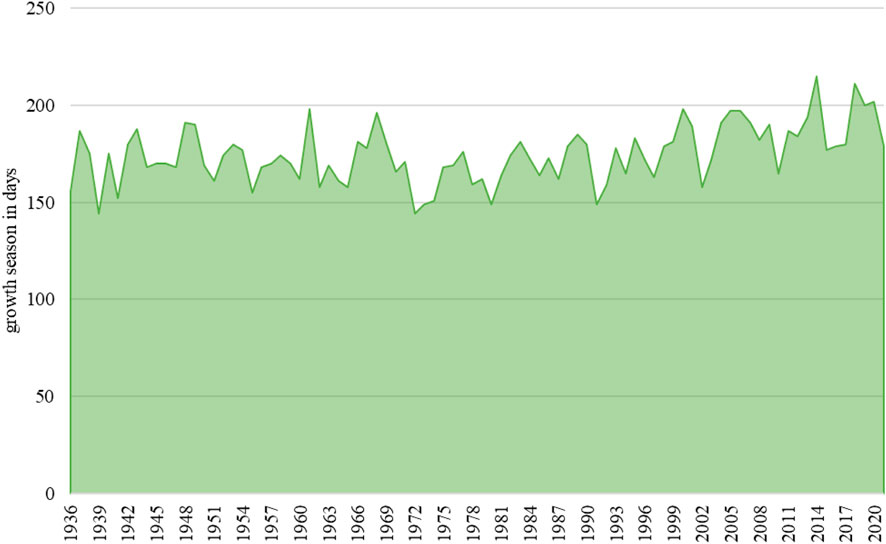
FIGURE 4. Visualization of the growing season.
The relative growth conditions in terms of local temperature gradients were determined as follows:
The precipitation was summed for the respective year and the corresponding vegetation period. This rainfall donation was distributed to a site-specific infiltration coefficient. The data were retrieved from the WFS download service using the Quantum GIS software and accessed the expansion of the city of Magdeburg in a tailored way. The calculation of the effective rainfall followed a simple approach based on the infiltration capacity of the respective location of the tree individual. The data from the LAGB were interpreted as follows:
The relative precipitation optimum was considered as follows:
Figure 5 shows the relative optimum in terms of annual precipitation. Next, the daily
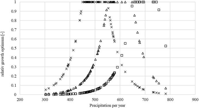
FIGURE 5. Visualization of the relative growth optimum
The next influencing factor in the water cycle is the uptake of groundwater (
It should be noted that at this stage, the previous function does not consider the influence of changing groundwater levels but rather the rootability of the soil.
This takes into account the factor for soil-dependent rootability (frs) and plant-specific rooting depth (SL). The soil compartment has a great influence on rootability. Accordingly, the average values from the official Soil Mapping Guidance (Sponagel, Grottenthaler, Hartmann et al., 2005) were used for the different soil types. A classification of the storage density of the soil was made to be able to estimate the air capacity and, also, the rooting depth accordingly. The storage density for parks and playgrounds was set to category 2, while that for street trees was set to category 4.
The reference evapotranspiration was estimated using the Hargreaves equation (Allen, Pereira, Raes et al., 1998).
Herein, the temperature was represented as the daily (index i) min, mean, and max at 2 m elevation above the ground in °C. The extraterrestrial solar radiation
The influence of tree growth competition was determined by the overlap of the crown projection area, assuming a 1:1 ratio between the crown and root space. This means that the projection surface corresponded to the area of the crown expansion. However, a uniform crown expansion was assumed. This is usually not the case as individual branches compete for light resources. This competitive situation affects the growing conditions. Depending on the ecological preference for lighting conditions, which can be estimated by the tree-specific indicator values, the growth and, thus, the pursuit of solar energy differ. According to the type of competition, it can be divided into different states, such as a one-sided advantage through the use of resources and mutual benefit (for example, shade plants in the shade of a light plant). For the next steps, each TOI (tree of interest) was assigned a position in the center of a coordinate system with the respective coordinate origin in the point
and for the vertical coordinate point as follows:
The distance from the TOI to the potential competitor was determined as follows:
Figure 6 shows how the position of the competitors affects the direct irradiation of the TOI in the context of the azimuth angle and the path of the sun (horizontal). The determined point coordinates of the respective competitor were used to calculate the azimuth angles using the following equation:
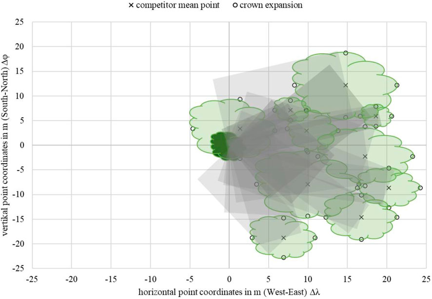
FIGURE 6. Example of the theoretic mean shading (gray) for Acer campestre with 10 competitors (TOI: ID 324 C: ID 304, 308, 309, 331, 332, 338, 357, 50612, 50613, 50614), metric-scaled.
The shading by the competitor, significantly influenced by the elevation angle of the two trees to each other, was determined using the tree heights and the distance as follows:
Finally, considering the azimuth angle and elevation angle, the effect of shading was determined. For this purpose, the course of the sun was set according to the definition of DIN5034 from Quaschning (2013).
A simple approach provides the approximate period during the day that the tree is shaded. For this purpose, the crown radius of the competitor was used to determine the minimum and maximum X and Y extent in the aforementioned coordinate system. The new equation for the minimum and maximum Y distance (North-South-Point coordinates) based on Equation 20 is shown as follows:
The further equation for the minimum and maximum X distances (West-East-Point coordinates) based on Equation 19 is shown as follows:
Next, the respective new point coordinates were converted into the corresponding azimuth angles by inserting them into Equation 22. From this followed the recalculation of the minimum and maximum azimuth angles in the north-south direction an exchange of the term
As shown in Figure 7, a daily or seasonally fluctuating disturbance impulse was associated with the numbers, height, crown dimension, and species of the competitors. For example, birch (e.g., Betula pendula) species have a lower leaf area than a same-sized oak (e.g., Quercus robur). Thus, only individuals who cut the path of the sun had influenced illuminance. The simplified hours of shading were set as follows to the sun elevation in the growing season:
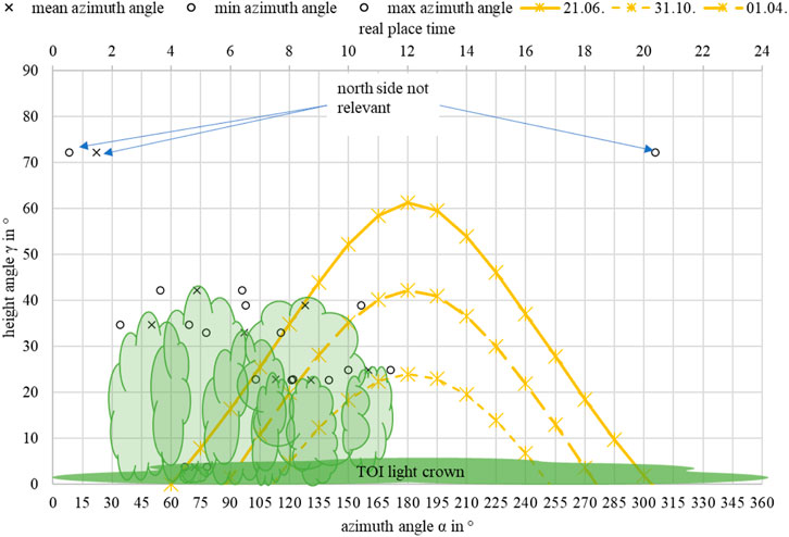
FIGURE 7. Example of the theoretic mean shading for Acer campestre with 10 competitors (TOI: ID 324; C: ID 304, 308, 309, 331, 332, 338, 357, 50612, 50613, 50614) based on the sun trajectory for the maximum vegetation period (01.04.–31.10.), including the height- and azimuth angles of the competitors.
The day of the year was set in the previous function as follows. Day 91 is April 1, while day 172 is the summer solstice (June 21). For the first period of the growing season, we used the dates described earlier. After June 21, the sun elevation decreases until the end of the growing season (day 304). Day 243 is August 31, during which the sun elevation is the same as that on April 1. The limits defined by the respective days in the year are provided with the following parameters:
The reduction of the solar radiation from shading by a competitor is summed for the TOI, as given in the following equation:
The reduction of solar radiation is considered as follows:
The incoming relativized solar radiation
For the rest of the procedures, the
The root space competition was determined by the screen projection surfaces. For this purpose, the tree cadaster (ESRI shape) was first expanded by the crown diameter and then blended with the already prepared individual layers of the examined tree species. The calculated area required all overlapping areas of the crown projections areas of the TOI and its corresponding competitors. Subsequently, the areas for the respective tree of interest were summed. The R extension package for QGIS, specifically the script “summarize by two fields”, was used to summarize the single overlay areas for all competitors to the TOI (
Assuming a crown-root ratio of 1:1, the root expansion from TOI was approximated, based on the crown diameter using the following equation.
The competitive pressure of the TOI and its corresponding competitors was considered according to Equation 33:
Parameterization by multiple regression analysis was performed as follows:
The individual parameters were related to general growth. For
The extent of the allometric relationships for the tree of interest is estimated after transformation as follows:
In the previous equation, the parameters
To interpret the prognosis results, we used the mean absolute error MAE and the root mean square error RMSE. With the MAE, the outliers in the database are not weighted as heavily as they are with the RMSE. Thus, a comparison of the two measures of accuracy (MAE and RMSE) of the estimators gives a good overview of the most suitable function for the respective parameters.
The MAE and RMSE were evaluated using rank analysis. The lowest MAE/RMSE was assigned the lowest rank; accordingly, ranks 2 to 9 were assigned in ascending order for increasing MAE/RMSE. The estimator with the lowest rank was assumed to have the best forecasting performance. This, in turn, allowed a conclusion to be drawn regarding the abiotic factors (temperature and precipitation). For all investigated allometric correlations, rank analysis was performed and the mean value was calculated over the respective results.
4 Results
4.1 Overview of the analysis results
Most of the Acer campestre (93.95%) trees were between 30 and 90 years of age. Young trees (≤30 years) and older (>90 years) comprised 4.42% and 1.63% of Acer campestre trees, respectively. A total of 82.61% of the trees were in parks and other public green spaces, whereas 17.39% were located beside roads. More than 52% of trees had a bhd of <32.5 cm. The street trees had an average bhd of 25.5 cm (sd ± 13.6 cm), an average height of 8.8 m (sd ± 3.2 m), and an average crown radius of 4.7 m (sd ± 2 m) with an average age of 41.8 years (sd ± 9.7 years). Trees in parks and other green infrastructure had an average bhd of 58.5 cm (sd ± 20.9 cm), an average height of 11.9 m (sd ± 4.4 m), and an average crown radius of 6.6 m (sd ± 3.2 m) at an average age 58.5 years (sd ± 27.4 years). The maximum bhd was 159.2 cm. The maximum height was 28 m, and the maximum crown diameter was 18 m. For further information, please refer to Figure 8.
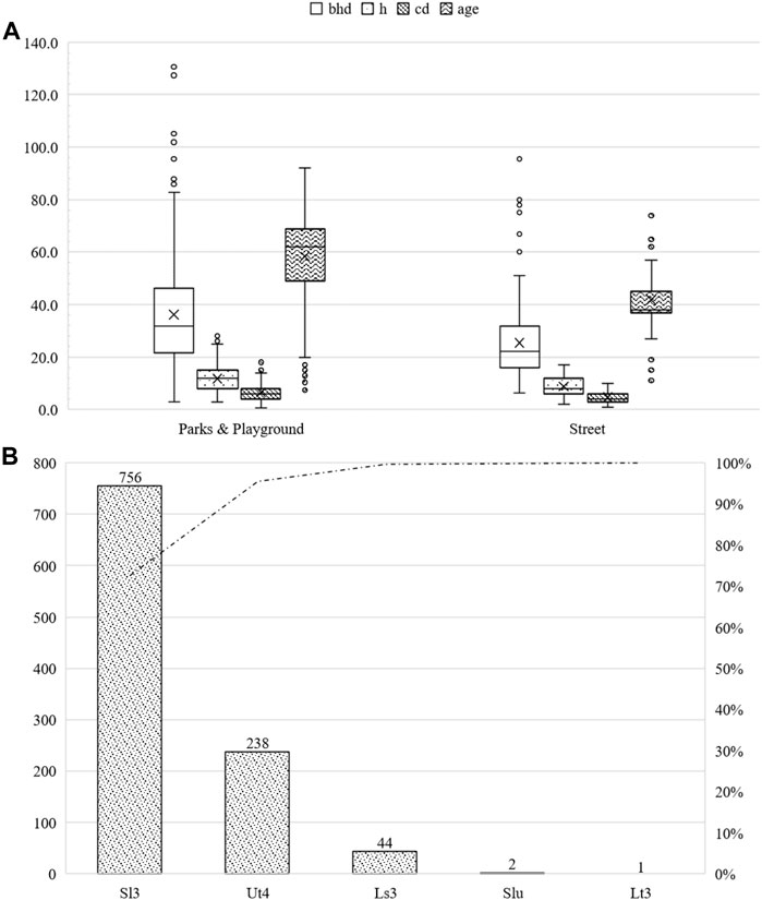
FIGURE 8. Summary of the studied Acer campestre subdivided into parks and other green areas, as well as roadside green areas. bhd in cm, h and cd in m, and age in years (A). Number of studied Acer campestre classified by soil type (B).
Similar to A. campestre, most trees (96.6%) of the species Acer platanoides were aged between 30–90 years. In contrast, young trees and trees >90 years of age accounted for 0.09%, and 2.61% of the trees, respectively. A total of 76.2% of the trees were located in parks and other green infrastructures, and the rest were street trees. The street trees had an average bhd of 36.9 cm (sd ± 12.5 cm), an average height of 11.8 m (sd ± 3.1 m), and an average crown radius of 8.5 m (sd ± 1.7 m) at an average age of 47.8 years (sd ± 15.1 years). Individuals in parks and other green infrastructure had an average bhd of 45.2 cm (sd ± 16.5 cm), an average height of 18.1 m (sd ± 4.2 m), and an average crown radius of 9.6 m (sd ± 2.9 m) at an average age of 64.2 years (sd ± 12.5 years). The maximum bhd was 167.1 cm, which represented the maximum height of 35 m, and the maximum crown diameter was 28 m. For further information, please refer to Figure 9.
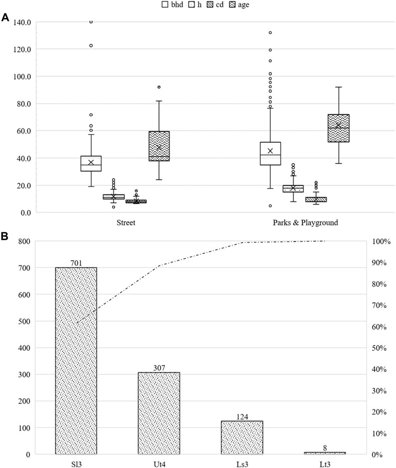
FIGURE 9. Summary of the studied Acer platanoides subdivided into parks and other green areas as well as roadside green areas. bhd in cm, h and cd in m and age in years (A). Number of studied Acer platanoides classified by soil type (B).
The most significant proportion of Malus spp. was younger than 30 years (60.9%). The rest of the trees was >30 years (31.1%). More than 51.1% of the trees were distributed on the streets. The rest were allocated in parks and other green infrastructures. The street trees had an average bhd of 26.3 cm (sd ± 5.9 cm), an average height of 3.8 m (sd ± 1.1 m), and an average crown radius of 2.3 m (sd ± 1.3 m) at an average age of 26.3 years (sd ± 11.6 years). Individuals in parks and other green infrastructure had an average bhd of 13.1 cm (sd ± 12.7 cm), an average height of 4.5 m (sd ± 2.0 m), and an average crown radius of 2.7 m (sd ± 2.1 m) at an average age of 25.9 years (sd ± 20.1 years). The maximum bhd was 79.6 cm, the maximum height was 16 m, and the maximum crown diameter was 12 m. For further information, please refer to Figure 10.
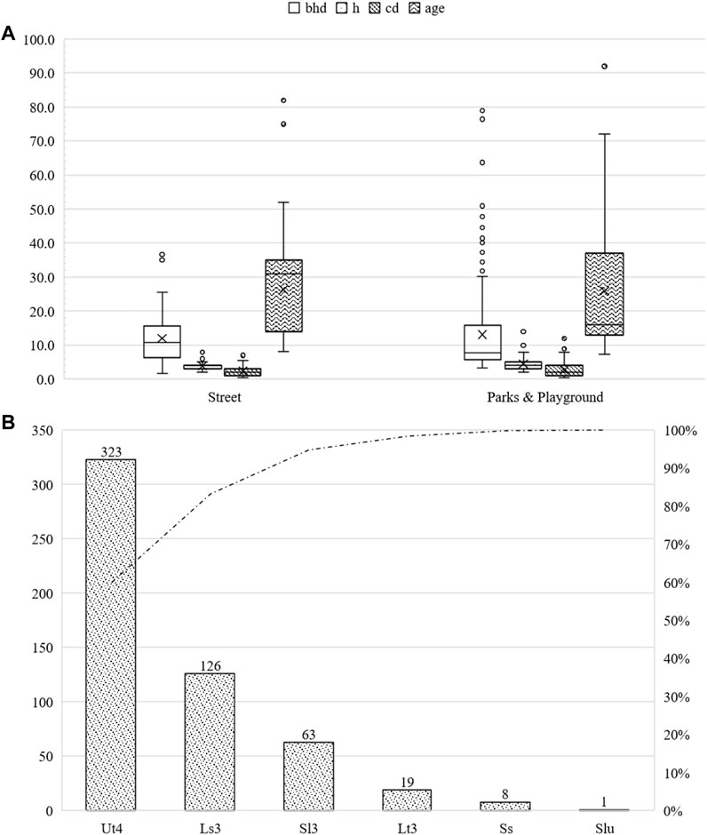
FIGURE 10. Summary of the studied Malus sp. subdivided into parks and other green areas, as well as roadside green areas. bhd in cm, h and cd in m, and age in years (A). Number of studied Malus sp. classified by soil type (B).
The largest proportion of Q. robur trees (78.4%) was 30–90 years of age, followed by those aged >90 years (93 specimens, 7.9%) and <30 years (160, 13.7%). A total of 23.3% of the trees were located in streets, while 76.7% were located in parks and other green infrastructure. The street trees had an average bhd of 27.6 cm (sd ± 11.5 cm), an average height of 9.8 m (sd ± 3.3 m), and an average crown radius of 5.3 m (sd ± 2.8 m) at an average age of 36.8 years (sd ± 12.4 years). Individuals in parks and other green infrastructure had an average bhd of 42.7 cm (sd ± 21.7 cm), an average height of 16.5 m (sd ± 6.9 m), and an average crown diameter of 8.0 m (sd ± 4.5 m) at an average age of 61.9 years (sd ± 22.8 years). The maximum bhd is 254.6 cm, which represented the threshold value. The maximum height was 35 m, and the maximum crown diameter was 25 m. For further information, please refer to Figure 11.
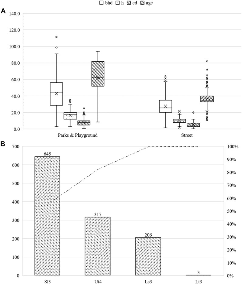
FIGURE 11. Summary of the studied Quercus robur subdivided into parks and other green areas, as well as roadside green areas. bhd in cm, h and cd in m, and age in years (A). Number of studied Quercus robur classified by soil type (B).
4.2 Acer campestre
The multiple regression results showed no significant relationship between temperature and bhd for all nine scenarios. Water uptake was identified as significant in eight of the nine scenarios. Only scenario 1 showed conditional significance (p-value = 0.059). The influence of competition could be detected in four of the nine scenarios.
Analogous to the bhd, no significance could be identified for h for the environmental parameter temperature. 6 of the 9 scenarios were significant compared to the water uptake. The competitive situation could be demonstrated for 2 of the 9 scenarios.
For crown diameter, the environmental factors of temperature and competition were significant for all scenarios. Water uptake was only relevant for scenario 1 (Figures 12–14).
FIGURE 12. Acer campestre breast height diameter measurements and growth prognoses based on the scenarios.
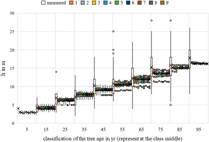
FIGURE 13. Acer campestre height measurements and growth prognoses based on the scenarios.
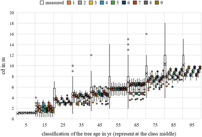
FIGURE 14. Acer campestre crown diameter measurements and growth prognoses based on the scenarios.
The nine scenarios studied had an MAE for bhd between 10.7539 cm (Rk(1)) and 10.7944 cm (Rk(9)); for h, the values were between 2.5029 m (Rk(1)) and 2.5129 m (Rk(9)); and for cd, between 1.7603 m (Rk(1)) and 1.8728 m (Rk(9)). The bhd was best described by scenario 9, and for h and cd, by scenarios 2 and 3. For all allometric relationships, the largest MAE (highest ranks 7–9) was indifferent. Changing the optimal conditions from scenario 3 to scenario 9 resulted in a 0.4 cm improvement in the MAE for bhd. Changing from scenario 9 to scenario 2 improved the h forecast by 0.01 m and changing from scenario 4 to scenario 3 improved the cd forecast by 0.11 m. Based on the averaging of the rank analysis, scenarios 2, 3, 6, and 9 emerged as the preferred abiotic optimum. Initially, there was no clear result. However, a preference for the temperature range between 19°C–21°C can be assumed.
The nine scenarios studied had an RMSE for bhd between 17.2444 cm (Rk(1)) and 17.3378 cm (Rk(9)); the RMSE values for h were between 10.7730 m (Rk(1)) and 10.8541 m (Rk(9)); and for cd, between 5.4569 m (Rk(1)) and 6.2500 m (Rk(9)). The bhd was best described by scenario 9, h by scenario 1, and cd by scenario 3. For all allometric relationships, the largest RMSE (highest ranks 7–9) was indifferent. Changing the optimal conditions from scenario 1 to scenario 9 resulted in a 0.09 cm improvement in the RMSE for bhd. Changing from scenario 9 to scenario 1 improved the h forecast by 0.08 m and changing from scenario 4 to scenario 3 improved the cd forecast by 0.79 m. Based on the averaging of the rank analysis, scenarios 3 and 9 emerged as the preferred abiotic optimums (Rk = 4.3333).
Overall, an optimal temperature between 21°C–23°C and annual rainfall between 650–750 mm can be derived for Acer campestre (Rk = 4.3333).
4.3 Acer platanoides
The multiple regression results for the bhd showed no significant scenario for all the relationships examined that were suspected to be influencing factors. In six of the nine scenarios, a significant correlation was evident for the environmental factor temperature. However, the correlation was not significant for the temperature range of 17°C–19°C (scenarios 1, 4, and 7). Water uptake was found to be significant in scenario 6. No significant correlation between competition and bhd growth could be determined in any scenario.
Multiple regression showed a significant relationship for temperature in all scenarios for the elevation forecast. Water uptake was identified as significant in scenarios 3, 5, 6, 8, and 9. While the competition was evident as conditionally non-significant (p-value = 0.069 and 0.058) for the elevation forecast only in scenarios 3 and 6, dependence was evident in all other scenarios.
For the prediction of crown diameter, no dependencies were demonstrated for scenarios 1–2, 4–5, and 7–8 with the environmental parameters. Scenarios 3, 6, and 9 showed significant correlations (temperature optimum 21°C–23°C in each case) with temperature. No significant relationship was found for any other environmental factors. For more information, please refer to Figures 15–17.
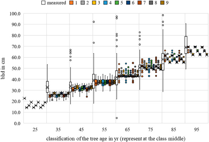
FIGURE 15. Acer platanoides breast height diameter measurements and growth prognoses based on the scenarios.
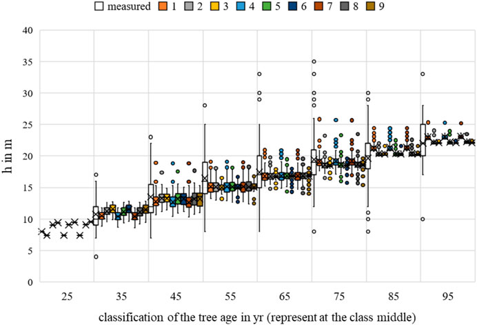
FIGURE 16. Acer platanoides height measurements and growth prognoses based on the scenarios.
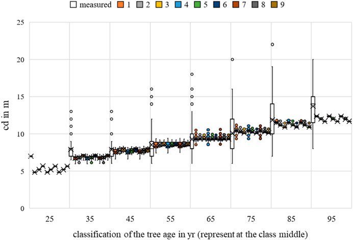
FIGURE 17. Acer platanoides crown diameter measurements and growth prognoses based on the scenarios.
The nine scenarios studied showed an MAE for bhd between 8.4055 cm (Rk(1)) and 8.7397 cm (Rk(9)); the MAE for h was between 2.6757 m (Rk(1)) and 2.7493 m (Rk(9)); and for cd, between 1.7117 m (Rk(1)) and 1.7462 m (Rk(9)). The bhd was best described by scenario 9, h by scenario 8, and cd by scenario 3. For all allometric relationships, the largest MAE (highest ranks 7–9) was observed for the temperature range between 17°C and 19°C set as the optimum. Changing the optimal conditions from scenario 1 to scenario 9 resulted in a 0.33 cm improvement in the MAE for bhd, to scenario 3 resulted in a 0.03 m improvement in the MAE for cd, and from scenario 1 to scenario 8 resulted in a 0.07 m improvement in the MAE for h. Based on the averaging of the rank analysis, scenario 9 emerged as the preferred abiotic optimum (Rk = 2.000).
The RMSE for bhd was between 13.2584 cm (Rk(1)) and 13.3810 cm (Rk(9)); while that for h was between 13.3414 m (Rk(1)) and 13.8996 m (Rk(9)), and for cd, between 5.4941 m (Rk(1)) and 5.5343 m (Rk(9)). The bhd was best described by scenario 9, h by scenario 8, and cd by scenario 1. For the allometric relationships, the largest RMSE (highest ranks 7–9) was indifferent. For the bhd, the largest RMSE (Rk(9)) was observed for scenario 7, and scenarios 3 and 9 for h and cd, respectively. Changing the optimal conditions from scenario 7 to scenario 9 resulted in a 0.12 cm improvement in the RMSE for bhd. Changing from scenario 1 to scenario 8 improved the h forecast by 0.56 m, and changing from scenario 9 to scenario 1 improved the cd forecast by 0.04 m. Based on the averaging of the rank analysis (Rk = 4.000), scenarios 2 and 5 emerged as the preferred abiotic optimums, followed by scenarios 8 and 9 (Rk = 4.3333).
Overall, an optimal temperature between 21°C–23°C and annual rainfall between 650–750 mm can be derived for Acer platanoides (Rk = 3.1667).
4.4 Malus spp
The multiple regression results for the bhd showed that no scenario was significant for all the relationships examined that were suspected to be influencing factors. In all scenarios, a significant correlation was identified for the environmental factor temperature. Water uptake was not significant in any of the nine scenarios (all p-values >0.3). Significant correlations between competition and bhd growth could be determined in scenarios 3, 6, and 9.
Multiple regression showed a significant relationship for temperature in all scenarios for the elevation forecast. Water uptake was identified as significant in scenarios 4–9. While competition was evident as conditionally non-significant (p-value = 0.054 and 0.056) for the elevation forecast only in scenarios 3 and 6, dependence was evident in all other scenarios.
For the prediction of crown diameter, no dependencies were demonstrated for scenarios 1, 4, and 7 with the environmental parameters. Scenarios 3, 6, and 9 show significant correlations (temperature optimum 21°C–23°C in each case) for the temperature and competitor situation. For more information, please refer to Figures 18–20.
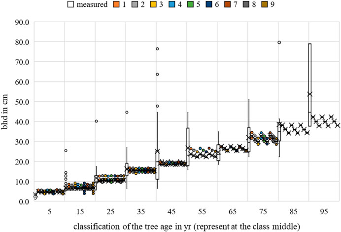
FIGURE 18. Malus sp. breast height diameter measurements and growth prognoses based on the scenarios.
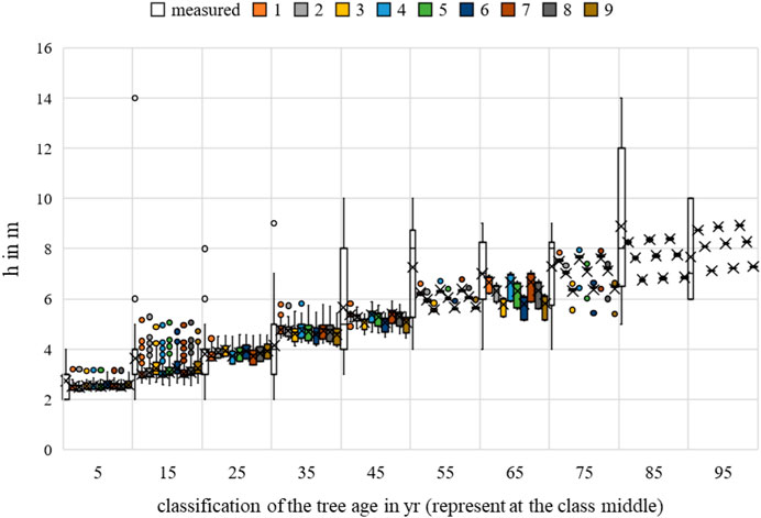
FIGURE 19. Malus sp. height measurements and growth prognoses based on the scenarios.
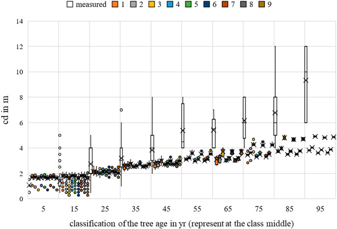
FIGURE 20. Malus sp. crown diameter measurements and growth prognoses based on the scenarios.
The MAE for bhd was between 2.9463 cm (Rk(1)) and 2.9728 cm (Rk(9)); for h, between 0.9523 m (Rk(1)) and 1.0055 m (Rk(9)); for cd, between 0.9565 m (Rk(1)) and 1.0793 m (Rk(9)). The bhd was best described by scenario 8, and h had the lowest MAE in scenario 9, while that for cd was observed in scenario 3. Changing the optimal conditions from scenario 6 to scenario 8 resulted in a 0.03 cm improvement in the MAE for bhd. Changing the optimal conditions from scenario 1 to scenario 9 resulted in a 0.05 cm improvement in the MAE for h. Changing the optimal conditions from scenario 4 to scenario 3 resulted in a 0.12 cm improvement in the MAE for cd. Based on the averaging of the rank analysis, scenarios 8 and 9 emerged as the preferred abiotic optimum (Rk = 3.3333).
The RMSE for bhd was between 5.9760 cm (Rk(1)) and 6.1134 cm (Rk(9)); for h, between 1.7951 m (Rk(1)) and 1.8434 m (Rk(9)); and for cd, between 1.6980 m (Rk(1)) and 2.1281 m (Rk(9)). The bhd was best described by scenario 7, and h had the lowest RMSE in scenario 8, while that for cd was observed in scenario 3. Changing the optimal conditions from scenario 3 to scenario 7 resulted in a 0.14 cm improvement in the RMSE for bhd. Changing the optimal conditions from scenario 1 to scenario 8 resulted in a 0.05 m improvement in the MAE for h. Changing the optimal conditions from scenario 4 to scenario 3 resulted in a 0.43 m improvement in the RMSE for cd. Based on the averaging of the rank analysis, scenario 8 emerged as the preferred abiotic optimum (Rk = 3.3333).
Overall, an optimal temperature between 19°C–21°C and annual rainfall between 650–750 mm can be derived for Malus sp. (Rk = 3.333).
4.5 Quercus robur
The multiple regression for height, breast height diameter, and crown diameter showed a generally significant relationship between the temperature and the allometric prognoses (p-value < 0.05). For crown diameter, dependence was evident in all scenarios for competition. None of the scenarios showed a significant correlation between growth and water uptake, with p-values < 0.05. The greatest significance of the parameter for the bhd and h forecast was identified for scenario 3, while that for the cd forecast was identified for scenario 1. For more information, please refer to Figures 21–23.
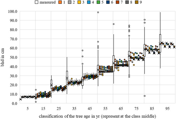
FIGURE 21. Quercus robur breast height diameter measurements and growth prognoses based on the scenarios.
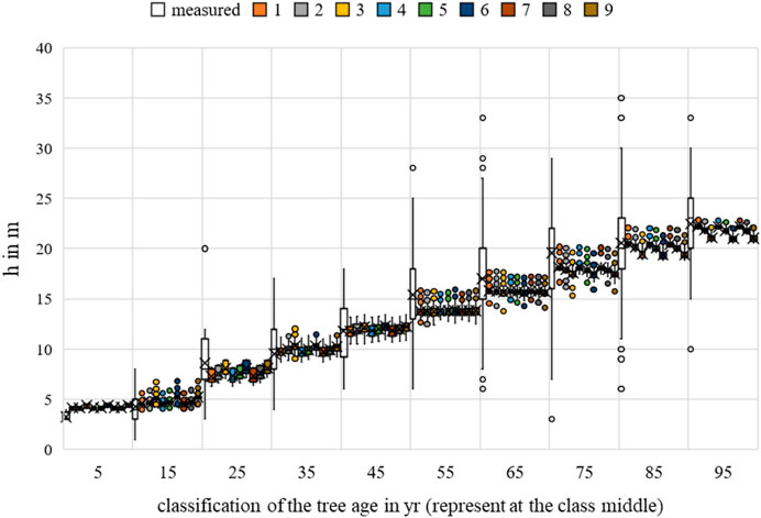
FIGURE 22. Quercus robur height measurements and growth prognoses based on the scenarios.
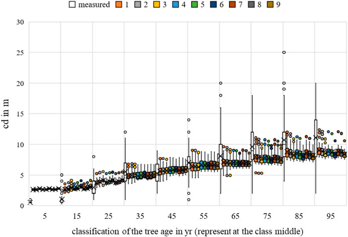
FIGURE 23. Quercus robur crown diameter measurements and growth prognoses based on the scenarios.
Regarding MAE, the value for bhd was between 8.0648 cm (Rk(1)) and 8.2698 cm (Rk(9)); for h, between 2.9605 m (Rk(1)) and 3.0428 m (Rk(9)); and for cd, between 2.4712 m (Rk(1)) and 2.5611 m (Rk(9)). The bhd was best described by scenario 8; h and cd had the lowest MAE in scenario 4. Changing the optimal conditions from scenario 9 to scenario 8 resulted in a 0.21 cm improvement in the MAE for bhd. Changing the optimal conditions from scenario 6 to scenario 4 resulted in a 0.08 m improvement in the MAE for h. Changing the optimal conditions from scenario 3 to scenario 4 resulted in a 0.09 m improvement in the MAE for cd. Based on the averaging of the rank analysis, scenarios 4 and 8 emerged as the preferred abiotic optimum (Rk = 2.3333).
The RMSE for bhd was between 12.0572 cm (Rk(1)) and 12.2529 cm (Rk(9)); for h, between 16.2062 m (Rk(1)) and 17.1118 m (Rk(9)); and for cd, between 11.8517 m (Rk(1)) and 12.5900 m (Rk(9)). The bhd was best described by scenario 7, while h and cd had the lowest RMSEs in scenario 1. Changing the optimal conditions from scenario 9 to scenario 7 resulted in a 0.20 cm improvement in the RMSE for bhd. Changing the optimal conditions from scenario 6 to scenario 1 resulted in 0.74 m and approximately 0.91 m improvements in the RMSEs for cd and h, respectively. Based on the averaging of the rank analysis, scenario 7 emerged as the preferred abiotic optimum (Rk = 1.6667).
Overall, an optimal temperature between 17°C–19°C and annual rainfall between 650–750 mm can be derived for Quercus robur (Rk = 2.000).
5 Discussion
The results of the regression showed a variety of relationships between allometric parameters and the abiotic environment. Trees in parks are generally smaller than those located on streets. Local climatic conditions could have caused this effect. The water uptake is often lower and the thermal conditions are often bitter, unlike trees in parks. This may be due to faster growth.
It was not possible to identify the expected correlations for all tree species. Consideration of the bhd in all nine scenarios for A. campestre showed that when approaching the limit value (0.6 in our example), the bhd decreased (negative coefficient). Since this coefficient was not significant in any scenario, a correlation between the temperature optimums chosen here must be discarded. However, it was evident that the water supply was important in many scenarios. A better water supply resulted in a larger bhd. Similarly, a better water supply meant less height growth. However, competition had a beneficial effect on height growth. Acer platanoides showed a significant correlation with bhd growth, especially in the scenarios with higher temperature optimum. Regarding height growth, competition resulted in a reduced height gain. Likewise, the effect of a lower height increased with a better water supply analogous to Acer campestre was also evident here. No significant correlations for an optimum temperature range between 17°C–19°C were observed. Malus sp. showed a significant correlation between bhd growth and temperature in all scenarios. A higher temperature encouraged greater growth. Precipitation was not significant in any scenario but showed a negative impact. The competition showed significant correlations with both bhd and height. Greater competition had an inhibiting effect on height growth. On the other hand, Q. robur showed significant correlations between temperature and bhd and altitude growth across all nine scenarios. Thus, a greater relative temperature optimum had a positive effect on growth. No significant correlations were observed for water supply.
To improve the forecast quality, further data are needed for verification. Furthermore, the growth function requires adjustment. Accordingly, the different phases of tree life can be used to adapt to the initial growth. Accordingly, better solutions can be achieved iteratively by extending the optimums or adjusting Equation 5. In addition, changing the weighting of the respective allometric relationship (thickness, height, and crown growth) can affect the results of the rank analysis. The crown growth of street trees is particularly influenced by regular pruning; thus, this growth is influenced by humans with recurring regularity.
6 Conclusion and outlook
Missing parameters that might further influence tree growth can be identified through future data collection. The implementation of sensor technology can be used to gain detailed knowledge of physiological responses to environmental changes and the potential associated effects on allometric contexts. A better prognosis for site-specific ecosystem services can be achieved when the growth characteristics are sufficiently known. In the future, by focusing on the provision of ecosystem services in municipal planning, the developed routines can be used for detailed sustainable urban greenery planning. The challenges to the application of sensor techniques to public green spaces might be theft and vandalism. The permanent installation of sensors in publicly accessible areas is also challenging.
The ecosystem performance of carbon sequestration is highlighted when trees act as urban carbon sinks. Oxygen is vital to most organisms. Photosynthesis is a crucial biochemical process that forms the basis for carbon sequestration. This process depends on the plant species, temperature, CO2, water uptake, and especially light consumption. If the corresponding parameters are collected from many trees of a certain species, existing knowledge can be upgraded. In particular, inherited adaptations to the respective site conditions during natural spread are interesting. Water uptake and temperature are easily quantifiable parameters. At this point, the related ecosystem services can be measured along with physiologically relevant parameters.
Further insights can be gained by measuring the solar radiation in the foliage at different heights and in the surrounding area. These measurements can be used to assess summer mortality. Moreover, statements regarding comfort can be made in this setting. The sensors must be integrated representatively with reference to the leaf area to identify corresponding relationships.
Foliage and crowns are essential components in determining the dust filtering potential. Leaf placement, integral roughness, and the porosity of the leaf area should be considered in detail. These measurements should be performed with a durable integrated dust sensor in tree crowns and with reference to the immediate environment. In addition, a regular sensor should be implemented to collect leaves. This can be followed by dry and wet quantification methods.
Cultural values are notoriously difficult to quantify. However, their impact on human well-being is undisputed. The flowering of Prunus serrulata can illustrate the importance of green infrastructure for social components. Avenues with these trees serve as popular photo motifs (own observation; see Figure 24 Holzweg-Magdeburg).

FIGURE 24. Prunus serrulata (land use: street) at flowering time, Source: Schneider.
However, urban trees might also cause disadvantages, allergies, and damage to gray infrastructure, which are nuisances for humans. The hazards resulting from trees are often announced in advance. A longer growing season and warmer conditions promote faster growth of individual trees and represent an additional stressor at the extrema. Particularly, the production of biogenic volatile organic compounds (BVOCs) is associated with stressful situations. If the highly complex language of trees can be deciphered, appropriate countermeasures would be more promising. In addition to chemical messengers in tree communication, inner cries provide truth signals. These noises are only perceptible in the ultrasonic range and are believed to be caused by the tearing of the water column (cavitation).
Overall, far-reaching findings have been obtained in recent years. However, many research questions remain to be addressed in the future, such as the impact of heavily anthropogenic soils on tree growth.
Data availability statement
The raw data supporting the conclusion of this article will be made available by the authors, without undue reservation.
Author contributions
Conceptualization: TF and PS; methodology: TF; software: TF; validation: TF; formal analysis: PS and TF; investigation: TF and PS; resources: TF; data curation: TF; writing—original draft preparation: TF; writing—review and editing: PS; visualization: TF; supervision: PS; project administration: PS; funding acquisition: PS. Both authors contributed to the article and approved the submitted version.
Funding
This publication was part of the research project UGI Plan funded by Germany’s Federal Office for Food and Agriculture, grant number 033R212C.
Acknowledgments
Taxonomy and nomenclature were guided by Jäger et al. (2021). The authors thank the urban planning department of the city of Magdeburg for data provision and fruitful scientific discussion. Moreover, the authors thank the reviewers for their valuable comments.
Conflict of interest
The authors declare that the research was conducted in the absence of any commercial or financial relationships that could be construed as a potential conflict of interest.
Publisher’s note
All claims expressed in this article are solely those of the authors and do not necessarily represent those of their affiliated organizations, or those of the publisher, the editors and the reviewers. Any product that may be evaluated in this article, or claim that may be made by its manufacturer, is not guaranteed or endorsed by the publisher.
Supplementary material
The Supplementary Material for this article can be found online at: https://www.frontiersin.org/articles/10.3389/fenvs.2023.1090652/full#supplementary-material
References
Allen, R.-G., Pereira, L.-S., Raes, D., and Smith, M. (1998). Crop evapotranspiration – guidelines for computing crop water requirements. Rome (Italy): FAO – Food and Agriculture Organization of the United Nations. 92-5-104219-5.
Baldacchini, C., Sgrigna, G., Tallis, M., and Calfapietra, C. (2019). An ultra-spatially resolved method to quali-quantitative monitor particulate matter in urban environment. Environ. Sci. Pollut. Res. Int. 26 (18), 18719–18729. doi:10.1007/s11356-019-05160-8
Bergmann, K.-C., and Straff, W. (2015). Klimawandel und Pollenallergie: Wie können Städte und Kommunen allergene Pflanzen im öffentlichen Raum reduzieren?. Umwelt und Mensch - Informationsdienst. Berlin: Federal Office for Radiation Protection, Federal Institute for Risk Assessment, Robert Koch Institute and Federal Environment Agency (ed.), 5–13.
Bongardt, B. (2006). “Stadtklimatologische Bedeutung kleiner Parkanlagen - dargestellt am Beispiel des Dortmunder Westparks,” in Essener ökologische schriften, bd. 24 (Hohenwarsleben: Westarp Wissenschaften).
Breckle, S.-W., and Rafiqpoor, M. D. (2019). Vegetation und Klima. Bielefeld. Bonn (Germany): Springer Spektrum. 978-3-662-59899-3. doi:10.1007/978-3-662-59899-3
Breuste, J. (2022). Die wilde Stadt: Stadtwildnis als Ideal, Leistungsträger und Konzept für die Gestaltung von Stadtnatur. Salzburg: Springer Nature. doi:10.1007/978-3-662-63838-5
Breuste, J., Pauleit, S., Haase, D., and Sauerwein, M. (2016). Stadtökosysteme: Funktionen, Management und Entwicklung. Salzburg, Freising. Berlin, Hildesheim: Springer Spektrum. doi:10.1007/978-3-642-55434-6
Flade, A. (2018). Zurück zur Natur? Erkenntnisse und Konzepte der Naturpsychologie. Hamburg: Springer Fachmedien Wiesbaden. doi:10.1007/978-3-658-21122-6
Gebhard, U. (2020). Kind und Natur: Die Bedeutung der Natur für die psychische Entwicklung. Hamburg: Springer Fachmedien Wiesbaden. doi:10.1007/978-3-658-01805-4
Georg August University Göttingen, Germany (n.d.). Forstbotanischer garten: Im reich der Bäume - ACER PLATANOIDES. [Online]. Available at: https://www.uni-goettingen.de/de/biologie+und+%C3%96kologie/16404.html#:∼:text=Der%20Spitzahorn%20bildet%20keine%20wirkliche,ein%20tiefgehendes%2C%20aber%20kompaktes%20Herzwurzelsystem (Accessed 10, 2022).
Gloor, S., and Göldi Hofbauer, M. (2018). “Der ökologische wert von Stadtbäumen bezüglich der Biodiversität,” in Jahrbuch der Baumpflege 2018 (Braunschweig: Haymarket Media), 33–48. 978–3–87815–257–6.
Hayat, A., Hacket-Pain, A. J., Pretzsch, H., Rademacher, T. T., and Friend, A. D. (2017). Modeling tree growth taking into account carbon source and sink limitations. Front. Plant Sci. 8, 1. doi:10.3389/fpls.2017.00182
Heise, P., and Hallermayr, S. (2022). Grüne Stadt - gesunder Mensch: Herausforderungen, Lösungsansätze und Handlungsfelder. Coburg, Munich (Germany): Springer Nature. doi:10.1007/978-3-662-65317-3
Jäger, E. J. (2017). Rothmaler: Exkursionsflora von Deutschland. Halle (Saale), Germany: Springer Spektrum. doi:10.1007/978-3-662-61011-4
Jahn, H. J., Krämer, A., and Wörmann, T. (2013). Klimawandel und Gesundheit: Internationale, nationale und regionale Herausforderungen und Antworten. Bielefeld: Springer Spektrum. doi:10.1007/978-3-642-38839-2
Kalusche, D. (2016). “Beleuchtung um 13 Uhr an klaren Tagen in verschiedener Höhe innerhalb eines Eichenwaldes,” in Ökologie in Zahlen - eine Datensammlung in Tabellen mit über 10.000 Einzelwerten. Editor D. Kalusche (Berlin, Heidelberg: Springer Spektrum). 978-3-662-47986-5.
Kardan, O., Gozdyra, P., Misic, B., Moola, F., Palmer, L. J., Paus, T., et al. (2015). Neighborhood greenspace and health in a large urban center. Sci. Rep. 5, 11610. doi:10.1038/srep11610
Kuttler, W. (2010b). Urbanes klima - teil 1. Umweltmeteorologie. Gefahrst. - Reinhalt. Luft 70, 378–382. Nr. 7/8.
Lei, Y., Li, H., Guo, J., Deussen, O., and Zhang, X. (2018). Tree growth modelling constrained by growth euqations. Comput. Graph. Forum 37, 239–253. doi:10.1111/cgf.13263
Lockow, K. W. (2022). Waldbestandsmessung - stichprobenverfahren - wachstumsmodellierung. Eberswalde: Springer Spektrum. doi:10.1007/978-3-662-63061-7
Lukaszkiewicz, J., and Kosmala, M. (2008). Determining the age of streetside trees with diameter at breast height-based multifactorial model. Mai: Arboriculture and Urban Forestry, 137–143. doi:10.48044/jauf.2008.018
McPherson, E. G., van Doorn, N. S., and Peper, P. J. (2016). Urban tree database and allometric equations. Albany, CA: U.S. Department of Agriculture, Forest Service, Pacific Southwest Research Station. doi:10.2737/PSW-GTR-253
Mehra, S.-R. (2021). Stadtbauphysik: Grundlagen klima-und umweltgerechter Städte. Stuttgart: Springer. doi:10.1007/978-3-658-30449-2
Moser, A., Rötzer, T., Pauleit, S., and Pretzsch, H. (2017). Stadtbäume: Wachstum, Funktionen und Leistungen - risiken und Forschungsperspektiven, Freisingen: Technische Universität München. Available online: https://www.waldwachstum.wzw.tum.de/fileadmin/publications/Moser_2018.pdf.
Müller, F., Ritz, C. M., Welk, E., and Wesche, K. (2021). Rothmaler Exkursionsflora von Deutschland - Gefäßpflanzen: Grundband. 22. Auflage. Dresden, Halle (Saale), Görlitz, Germany: Springer Spektrum. doi:10.1007/978-3-662-61011-4
Quaschning, V. (2013). Regenerative energiesysteme: Technologie – berechnung – simulation. Berlin (Germany): Hanser Verlag München. 978-3-446-43526-1.
Riedel, T., Hennig, P., Kroiher, F., Polley, H., Schmitz, F., and Schwitzgebel, F. (2017). Die dritte bundeswaldinventur: BWI 2012. Eberswalde: Johann Heinrich von Thünen-Institut für Waldökosysteme. Available online: https://www.bundeswaldinventur.de/fileadmin/SITE_MASTER/content/Downloads/BWI_Methodenband_web.pdf.
Riedel, T., and Kändler, G. (2017). Nationale Treibhausgasberichterstattung: Neue Funktionen zur Schätzung der oberirdischen Biomasse am Einzelbaum. Eberswalde, Freiburg: DLV GmbH. doi:10.4432/0300-4112-88-31
Riffel, A. (2021). Heilpflanzen der Traditionellen Europäischen Medizin: Wirkung und Anwendung nach häufigen Indikationen. Mariazell: Springer Verlag. doi:10.1007/978-3-662-53724-4
Snorrason, A., and Einarsson, S. F. (2006). Single-tree biomass and stem volume functions for tree species used in Icelandic forestry. Icel. Agric. Sci. 19, 15–24.
Sponagel, H., Grottenthaler, W., Hartmann, K.-J., Hartwich, R., Janetzko, P., Joisten, H., et al. (2005). Bodenkundliche kartieranleitung. Hannover (Germany): Bundesanstalt für Geowissenschaften. 978-3-510-95920-4.
StMELF (2022a). Kurzbeschreibung heimischer Gehölze: Apfelbäume./Brief description of native woody plants: apple trees. [Online]. Available at: https://www.lfl.bayern.de/iab/kulturlandschaft/182146/index.php (Accessed Oktober, 2022).
StMELF (2022b). Kurzbeschreibung heimischer gehölze: Feld-ahorn./Brief description of native woody plants: field maple. [Online]. Available at: https://www.lfl.bayern.de/iab/kulturlandschaft/179406/index.php (Accessed Oktober, 2022).
StMELF (2022c). Kurzbeschreibung heimischer gehölze: Spitz-ahorn./Brief description of native woody plants: norway maple. [Online]. Available at: https://www.lfl.bayern.de/iab/kulturlandschaft/180600/index.php (Accessed Oktober, 2022).
StMELF (2022d). Kurzbeschreibung heimischer gehölze: Stiel eiche./Brief description of native woody plants: german oak. [Online]. Available at: https://www.lfl.bayern.de/iab/kulturlandschaft/151477/index.php (Accessed Oktober, 2022).
Thomas, F. (2018). Grundzüge der Pflanzenökologie. Trier (Germany): Springer Spektrum. 978-3662541388. doi:10.1007/978-3-662-54139-5
Keywords: urban tree growth, urban green infrastructure, urban planning, ecosystem services, plant physiology
Citation: Fauk T and Schneider P (2023) Modeling urban tree growth as a part of the green infrastructure to estimate ecosystem services in urban planning. Front. Environ. Sci. 11:1090652. doi: 10.3389/fenvs.2023.1090652
Received: 05 November 2022; Accepted: 09 May 2023;
Published: 08 June 2023.
Edited by:
Cristina Maria Monteiro, Escola Superior de Biotecnologia—Universidade Católica Portuguesa, PortugalReviewed by:
Debora Lithgow, Instituto de Ecología (INECOL), MexicoAnlur Lohachab, University of Tasmania, Australia
Rahim Alhamzawi, University of Al-Qadisiyah, Iraq
Copyright © 2023 Fauk and Schneider. This is an open-access article distributed under the terms of the Creative Commons Attribution License (CC BY). The use, distribution or reproduction in other forums is permitted, provided the original author(s) and the copyright owner(s) are credited and that the original publication in this journal is cited, in accordance with accepted academic practice. No use, distribution or reproduction is permitted which does not comply with these terms.
*Correspondence: Tino Fauk, dGluby5mYXVrQGgyLmRl