Assessment of groundwater quality in a highly urbanized coastal city using water quality index model and bayesian model averaging

Prediction and assessment of water quality are important aspects of water resource management. To date, several water quality index (WQI) models have been developed and improved for effective water quality assessment and management. However, the application of these models is limited because of their inherent uncertainty. To improve the reliability of the WQI model and quantify its uncertainty, we developed a WQI-Bayesian model averaging (BMA) model based on the BMA method to merge different WQI models for comprehensive groundwater quality assessment. This model comprised two stages: i) WQI model stage, four traditional WQI models were used to calculate WQI values, and ii) BMA model stage for integrating the results from multiple WQI models to determine the final groundwater quality status. In this study, a machine learning method, namely, the extreme gradient boosting algorithm was also adopted to systematically assign weights to the sub-index functions and calculate the aggregation function. It can avoid time consumption and computational effort required to find the most effective parameters. The results showed that the groundwater quality status in the study area was mainly maintained in the fair and good categories. The WQI values ranged from 35.01 to 98.45 based on the BMA prediction in the study area. Temporally, the groundwater quality category in the study area exhibited seasonal fluctuations from 2015 to 2020, with the highest percentage in the fair category and lowest percentage in the marginal category. Spatially, most sites fell under the fair-to-good category, with a few scattered areas falling under the marginal category, indicating that groundwater quality of the study area has been well maintained. The WQI-BMA model developed in this study is relatively easy to implement and interpret, which has significant implications for regional groundwater management.

1 Introduction

Sustainable management of water resources is a major challenge worldwide. With economic development and accelerated urbanization, water resources and supply are in increasing demand. Groundwater is an important water resource, and approximately 50% of the urban population worldwide has been estimated to draw water from groundwater (United Nations, 2022). Despite the abundance of groundwater, various problems, such as groundwater quality degradation, have increased with increasing population and water demand. Drinking contaminated groundwater has been reported to cause various health problems, including cholera, diarrhea, dysentery, and skin infections (Li and Wu, 2019). Therefore, it is important to assess the quality of groundwater as a water supply resource.

The research progress of WQI models has been extensive, with various models being developed, tested, and applied to different water bodies (Ibn Ali et al., 2020; Wu et al., 2021). Some of the traditional models include the National Sanitation Foundation (NSF) index, Weighted Quadratic Mean (WQM), Scottish Research Development Department (SRDD) index, and West Java (WJ) index (Uddin et al., 2021). Traditional WQI models are generally simple and easy to use. They provide a simple numerical value for assessing water quality, which can be used to compare different areas or to provide a general assessment of the water quality. However, the accuracy of the WQI model is limited due to its inability to take into account all the factors that may affect water quality. Additionally, the models may be difficult to interpret in certain cases, as they may not provide clear guidance on what actions should be taken in order to improve water quality (Sutadian et al., 2015). Recently, researchers have developed WQI models based on machine learning (ML) methods, such as Support Vector Regression and Decision Tree Regression (Asadollah et al., 2021). ML based methods are advantageous over traditional methods as they can provide accurate results with less human effort and time. In addition, ML based methods are able to detect hidden patterns and correlations in the data, which can be used to better understand water pollution sources and develop effective management strategies. However, WQI-ML models, on the other hand, are more complex and require more data (Lap et al., 2023).

WQI models usually consist of four major structural elements: parameter selection, parameter weight assignment, sub-index generation, and aggregation. However, these four elements may lead to model uncertainty because the selection of water quality parameters is based on actual needs or concerns, while the assignment of weights is mainly based on expert empirical methods without any system rules. Sub-index generation and aggregation have been developed based on local guidelines, resulting in many region-specific models (Tomas et al., 2017; Bilgin, 2018; Abdelaziz et al., 2020). Moreover, diversity in the sub-index and aggregation functions leads to differences in the final water quality evaluation results.

Many methods quantify model uncertainty using statistical analyses and/or expert judgment (Lowe et al., 2017). Bayesian model averaging (BMA) is an intuitive and attractive solution for quantifying model uncertainty (Hoeting et al., 1999). BMA provides a coherent mechanism for quantifying the overall uncertainty of the multi-model structure and parameters for model uncertainty. Some studies investigating the effects of different parameter selections, aggregation functions, and weight allocation processes on the final WQI values have reported that the WQI values vary over a wide range (Sutadian et al., 2017; Wu et al., 2018; Nong et al., 2020; Pan et al., 2022). Classification of water quality evaluation grades is based on the WQI values, which may confuse the decision maker or render the values unusable for decision-making. Therefore, it is important to reduce this uncertainty from the WQI water quality model.

In this study, we developed a WQI-BMA model for groundwater quality assessment. The model comprised two stages. First stage involved the construction of four traditionally used WQI models to assess the water quality. The results from these WQI models were then merged using BMA to quantify the inherent uncertainty of the WQI models and obtain the final calculation of groundwater quality. Groundwater quality data from the coastal city of Shenzhen, China from 2015 to 2021 were used to demonstrate the application of this model, assess the groundwater quality status, and study its spatio-temporal variations in the city. This WQI-BMA model can account for the uncertainty of multiple WQI models and provide a quantitative and comprehensive groundwater quality assessment. Therefore, the developed model and results of this study have important implications for the sustainable management of regional groundwater quality and water resources.

2 Materials and methods

2.1 Study site

Shenzhen is a coastal city located in southeast China, Guangdong Province, lying between 113°46′–114°37′E and 22°27′–22°52′N (Figure 1). The study region included 11 watersheds covering approximately 2000 km² area (Qiu et al., 2022). The region has a subtropical marine monsoon climate with an annual average precipitation of 1,830 mm. Precipitation is mainly concentrated from April to October, accounting for approximately 85% of the annual rainfall (Shenzhen Statistics Bureau, 2020). The study area terrain was high in the southeast and low in the northwest, mostly in low-hilly areas with gentle terraces. Groundwater types include quaternary loose deposits, pore water, bedrock fissure water, and karst water. The groundwater level was shallow and generally in the range of 1.5–4.5 m.

FIGURE 1

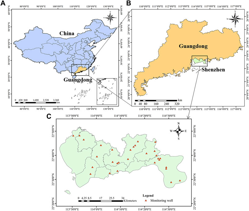
FIGURE 1. Location of the study area (A, B) and distribution map of the groundwater monitoring wells (C).

2.2 Data source

Groundwater quality data used in this study were obtained from the Water Authority of Shenzhen Municipality (http://swj.sz.gov.cn/). Water samples were collected from 30 monitoring wells in the study area from 2015 to 2021, covering the wet and dry seasons (684 samples; Supplementary Table S1). In this study, March and December represented dry season. June and September represented wet season. Locations of the sampling points are shown in Figure 1. The groundwater quality data included levels of pH, total dissolved solids (TDS), total hardness (TH), chloride (Cl⁻), fluoride (F⁻), ammonia-nitrogen (NH₃-N), nitrate (NO₃-N), nitrite (NO₂-N), sulphate (SO₄^2–), arsenic (As), total iron (Fe), total manganese (Mn), lead (Pb), cadmium (Cd), mercury (Hg), and dissolved oxygen (DO). Thirty monitoring wells were uniformly distributed throughout the study area.

2.3 WQI-BMA model

Figure 2 shows the framework of the WQI-BMA model integrating four traditionally used WQI models based on the BMA method to assess groundwater quality. In this framework, the implementation of the WQI-BMA model involves two stages. First stage involved the construction of four traditionally used WQI models as members of the BMA. In the first stage, the groundwater quality parameters were determined. All measurable groundwater quality parameters were used for comprehensive groundwater quality assessment. Once the groundwater quality parameters were determined, a machine learning approach, called the extreme gradient boosting algorithm, was used to systematically assign weights based on the rank order centroid weight method. The sub-index functions are then calculated based on a uniform calculation rule. The final step was to calculate the aggregation functions based on the four WQI models, and the results were then used for stage two, BMA merging. In stage two, BMA merged the four WQI models from stage one to quantify their uncertainty and provide a final groundwater quality assessment. By combining WQI methods and Bayesian model, the WQI-BMA model can provide more accurate and reliable predictions of water quality. This is due to the fact that the WQI-BMA model combines the strengths of multiple WQI models. The Bayesian model can take into account the uncertainty of the WQI models, which can be used to generate more accurate predictions. Additionally, the WQI-BMA model is more robust and less sensitive to outliers than any single WQI model.

FIGURE 2

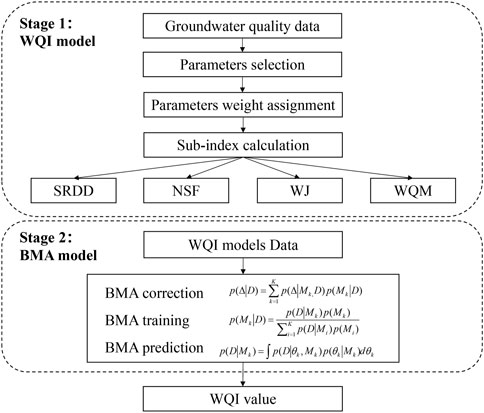
FIGURE 2. Framework of the water quality index (WQI)-Bayesian model averaging (BMA) model.

2.4 WQI models

WQI models are widely used tools for assessing the water quality. They can analyze large amounts of temporally and spatially varying water quality data to inform decision-makers about the water quality. The construction of a WQI model typically involves four steps. First step is to collect and analyze the water quality data to determine the number of parameters needed to evaluate the water quality. In the second step, parameter weights are assigned based on the importance of the water quality. In the third step, these parameters are normalized to a 0–100 scale using sub-index functions. Finally, the normalized sub-indices and parameter weights are combined into an overall WQI value using a suitable aggregation function, and the water quality is inferred using a classification scheme that defines the water quality classes.

Parameter selection is the first step for the WQI model. The parameters are usually selected based on data availability, expert opinion, and the environmental impact of water quality (Gupta and Gupta, 2021). In this study, 16 parameters that commonly reflect the water quality were considered for the WQI models. These 16 parameters included the levels of pH, TDS, DO, TH, Cl⁻, F⁻, NH₃-N, NO₃-N, NO₂-N, SO₄^2–, and heavy metals (As, Fe, Mn, Pb, Cd, and Hg).

Parameter weight is a key component of WQI models. It is typically determined based on the environmental importance of the groundwater quality parameters, together with the recommended guidance value. Such parameter weight allocations are usually biased towards the subjectivity of experts and do not follow any systematic technique. In this study, an objective weighting approach based on machine learning (ML) (Uddin et al., 2022) was employed to assign weights to groundwater quality parameters. This approach differs from the subjective approach used in the literature (e.g., expert opinion) and aims to reduce the uncertainty caused by inappropriate weighting. Two processes are involved in the objective weighting approach: i) extreme gradient boosting (XGBoost) ranking of the parameter, and the ii) rank order centroid (ROC) weight method, which attributes weightings based on rank.

ML can quantify the importance of input variables based on their influence on model output variables (Uddin et al., 2022). Similarly, it can be used to quantify the importance of water quality parameters. In this study, 16 water quality parameters at 30 monitoring wells were used as inputs for the ML model, and the corresponding groundwater quality status estimated based on the Environmental Quality Standards for Surface Water (GB3838-2017) was used as the output. Then, an initial assessment was conducted using several ML methods according to 5-folds of the k-fold cross-validation, including decision tree (DT), random forest (RF), naive Bayes (NB), extremely randomized trees (ERT), and XGBoost algorithms. All ML methods in this study were applied using Python-based open-source scikit-learn codes.

In this study, an approach combining the XGboost and ROC weight methods was used to assign weights to provide a better allocation than the expert opinion method (Uddin et al., 2021; Uddin et al., 2022). XGBoost is a widely used ensemble ML method based on the gradient boosting algorithm (Zhu et al., 2022). Some studies have used XGBoost to extract key variables, including water quality (Naghibi et al., 2020), air pollution (Li et al., 2022), and wastewater treatment (Wang D. et al., 2022), for developing new models. XGBoost has lower prediction errors than other algorithms as its regularized boosting technique controls the complexity of the model and prevents overfitting by adding regularization terms to the loss function. XGBoost can rank features based on their relative importance using SHapley Additive exPlanations (SHAP) values. SHAP values are local interpretation methods that provide more detailed, additional, and individualized explanations and attributions than global interpretation techniques (Li, 2022). This study ranked the relative importance of the groundwater parameters based on XGBoost and SHAP methods for subsequent weight calculations.

Hyperparameters are important for determining the structure and prediction accuracy of the model. In this study, grid search optimization method (Abbaszadeh et al., 2022) was used to determine the hyperparameters in the XGBoost model to achieve high prediction accuracy. XGBoost performance was evaluated using the accuracy and R² of the training and test datasets, where the input data were randomly divided into two groups: 80% of training dataset and 20% of testing dataset.

ROC weight method estimates the weights that minimize the maximum error of each weight by identifying the centroids of all possible consequences, while maintaining the rank order of objective importance. ROC weights of a set of n variables ranked from j = 1 to n were calculated using the following equation (Roszkowska, 2013):

$w_j=\frac{1}{n}{\displaystyle \sum }_{i=j}^n\frac{1}{r_i}(1)$

where w_j is the jth weight and r_i is the rank position of w_j.

Sub-index converts the measured groundwater quality values into unitless values. Sub-index values (q_j. ranging from 0 to 100) were obtained using the Delphi technique (Bordalo et al., 2001), which was used to indicate whether the variable had a poor or good status. In this study, the linear interpolation rescaling approach by Uddin et al. (2022) was used to compute the sub-index for all groundwater variables using Eqs. (2) and (3):

$q_j=\left(S{I}_u-S{I}_l\right)-\frac{\left(S{I}_u*C_j\right)}{\left(SI{T}_u-SI{T}_l\right)}(2)$

$q_j=\frac{\left(C_j-SI{T}_l\right)}{\left(SI{T}_u-SI{T}_l\right)}*S{I}_u(3)$

where SI_l and SI_u are the lower and upper limits of the possible q_j values (0 and 100, respectively); SIT_l and SIT_u are the lower and upper threshold values, respectively; and C_j is the measured value of the water quality parameter. Threshold guidelines are listed in Supplementary Table S2.

Final step of the WQI model involves the aggregation function, which converts multiple water quality parameters into a single value to express the overall water quality status. Several studies have shown that different results from different WQI models are related to the aggregation function (Lumb et al., 2011; Juwana et al., 2016; Ma et al., 2020). In this study, we considered four common traditional weighted aggregation functions in the WQI models: NSF, WQM, SRDD and WJ (Table 1). The output of the final WQI model was recommended for the four water quality classes listed in Table 2, according to Uddin et al. (2022). A WQI value in the range of 0–29 indicates that the water quality is very poor, and the water cannot be used for any purpose. A WQI value in the range of 30–49 indicates that the water can only be used for a small number of specific cases, with a high the risk of water pollution. A WQI value in the range of 50–79 indicates that the water body has minor pollution, with some indicators meeting the water quality standards. A WQI value in the range of 80–100 indicates that the water quality is good, satisfying most of the water quality standards.

TABLE 1

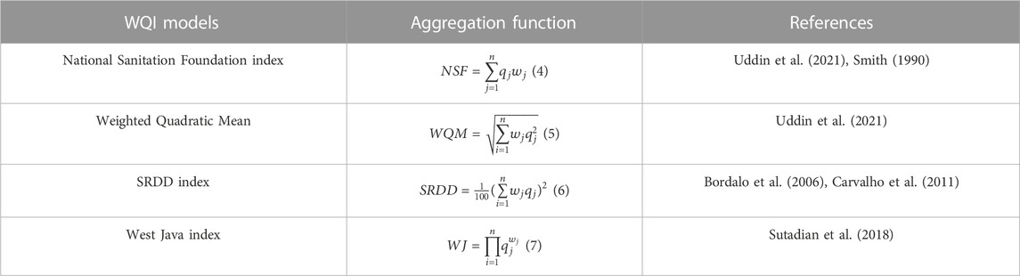
TABLE 1. Overview of four water quality index (WQI) model aggregation functions.

TABLE 2

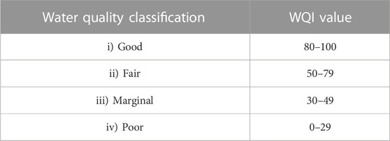
TABLE 2. Classification of water quality based on WQI values.

2.5 BMA

BMA is a statistical method for multi-model ensembles that has higher reliability and accuracy than the single-model method (Duan et al., 2007). BMA results are usually better than those of single models in terms of skill and reliability (Ashofteh et al., 2022). BMA has been used in many studies for groundwater vulnerability assessment (Gharekhani et al., 2022), mortality forecasting (Ashofteh et al., 2022), soil moisture estimation (Chen et al., 2020), merging of precipitation products (Yumnam et al., 2022), and streamflow simulation (Wang J. et al., 2022). BMS is a free R package for performing BMA using the open-source software R. In this study, the BMA model was applied using the BMS package in R version 4.1.2. For more information refers to BMS package is available at http://bms.zeugner.eu.

Based on Bayes’ theorem and the total probability law, posterior distribution of the BMA predicted quantities Δ) for the given data D) is (Hoeting et al., 1999):

$p\left(\Delta \left|D\right.\right)={\displaystyle \sum }_{k=1}^{K}p\left(\Delta \left|M_{k,}D\right.\right)p\left(M_k\left|D\right.\right)(4)$

where p (Δ|D) is the probability of the prediction of data Δ) given the observed data D); p (Δ|M_k,D) is the conditional probability of the predicted quantity given the observed data D) and given model (M_k), which is the output of SRDD, NSF, WJ, and WQM models; and p (M_k|D) is the posterior probability of the model given the data D), which is the model weight. Posterior probability of the model (M_k) is calculated using the following equation (Gharekhani et al., 2022):

$p\left(M_k\left|D\right.\right)=\frac{p\left(D\left|M_k\right.\right)p\left(M_k\right)}{{\sum }_{i=1}^{K}p\left(D\left|M_i\right.\right)p\left(M_i\right)}(5)$

where,

$p\left(D\left|M_k\right.\right)=\int p\left(D\left|{\theta }_k,M_k\right.\right)p\left({\theta }_k\left|M_k\right.\right)d{\theta }_k(6)$

Here, p (D|M_k) is the integrated likelihood of model M_k; θ_k is the vector of parameters of model M_k; p (θ_k|M_k) is the prior density of θ_k under model M_k; p (D|θ_k, M_k) is the likelihood, and p (M_k) is the prior model probability for the model M_k.

3 Results and discussion

3.1 Statistical analysis of groundwater quality variables

Statistical analysis results of the groundwater quality parameters in the study area are listed in Table 3. The parameters include many variables, such as the minimum value (Min), maximum value (Max), mean, standard deviation (SD), and coefficient of variation (CV). NH₃-N concentration values ranged from 0 to 56.40 mg/L with a mean value of 1.40 mg/L, which exceeds the limit of 0.5 mg/L set by the World Health Organization. pH varied from 5.14 to 8.60 with a mean value of 6.84, indicating that most groundwater within the study area was slightly acidic. Mean concentrations of As, Fe, and Mn were 0.012, 0.49, and 0.20 mg/L, respectively. Mean concentrations of the other parameters in the groundwater were less than the thresholds proposed in the WHO and Environmental Quality Standards for Surface Water (GB3838-2002) guidelines (Supplementary Table S2). CV for heavy metals ranged from 618.94% to 140.70% in the order As > Pb > Fe > Cd > Mn > Hg, indicating a large difference in the distribution of heavy metals in groundwater. SD of the groundwater quality data indicated high variability; therefore, variation in the mean value of the data was also high (Elbeltagi et al., 2022).

TABLE 3

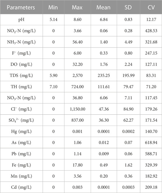
TABLE 3. Statistical analysis results of the groundwater quality parameters in the study area.

3.2 Performance of XGBoost

Supplementary Table S3 lists the findings of an initial assessment conducted using several ML methods (DT, RF, NB, ERT, and XGBoost) according to 5-folds of the k-fold cross-validation. Accuracy is a metric for evaluating ML classification problems and indicates the ratio of all correctly classified samples to the total number of samples. Among the 4 ML methods, the XGBoost model exhibited the highest prediction accuracy (83%). Prediction accuracies of DT (82%), RF (82%), ERT (77%), and NB (65%) were slightly lower than that of XGBoost. Thus, the XGBoost model was selected to rank the parameters according to the relative importance of the selection of important groundwater quality parameters. Table 4 lists the final adjusted hyperparameter values for the XGBoost model obtained using the grid-search optimization method. Combination of the hyperparameters in Table 4 resulted in the highest R² and accuracy in the predicted and observed values. A maximum tree depth of seven and a learning rate of 0.1 were used to increase the maximum effect of interactions between variables. The training and testing accuracies of the XGBoost model were 1 and 0.95, respectively, and the training and testing R² were 0.99 and 0.92, respectively. Results of the selection of important groundwater quality parameters using the XGBoost model integrated with SHAP values are shown in Supplementary Figure S1. At the study site, the most important factors influencing the water quality status were NH₃-N and Mn (Supplementary Figure S1). The order of importance of the groundwater parameters was NH₃-N > Mn > pH > NO₃-N > TDS > Pb > Fe > As > Hg > DO > SO₄^2– > Cd > Cl⁻ > F⁻ > TH > NO₂-N.

TABLE 4

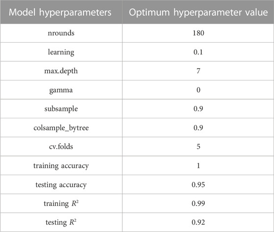
TABLE 4. Optimized extreme gradient boosting (XGBoost) algorithm hyperparameter values.

Table 5 lists the weight values of the groundwater quality parameters calculated using the ROC method. Weight values followed the same order as the rankings of the groundwater quality parameters, with NH₃-N, Mn, and pH exhibiting the highest weight values and F⁻, TH, and NO₂-N exhibiting the lowest weight values.

TABLE 5

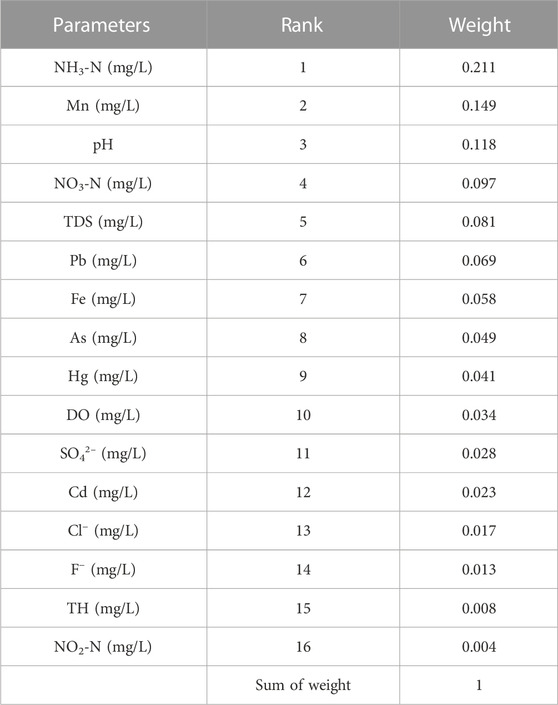
TABLE 5. Ranks and weight values of groundwater quality parameters.

3.3 Performance of the WQI-BMA model

In this study, four WQI models based on different weighted aggregation functions were used to calculate WQI values and infer the groundwater status. Figure 3 shows the range of the WQI values calculated for each function within the study area. Overall, there were significant differences in the WQI values obtained using different WQI models (Figure 3). WQM provided the smallest distribution of scores and the highest mean score. Conversely, WJ provided the largest distribution of scores and the lowest mean score. The mean score for NSF was lower than that for WQM but greater than that for SRDD. For the NSF and WQM models, the groundwater quality evaluation grade was higher than that for the SRDD and WJ models. In addition, most of the groundwater quality in the study area was above the grade “poor,” indicating that the groundwater quality in the study area was in the marginal to good level. In this study, all WQI models used the same groundwater quality parameters and sub-index functions, except the aggregation function, to calculate the WQI values. Therefore, the differences were caused by the different aggregation functions.

FIGURE 3

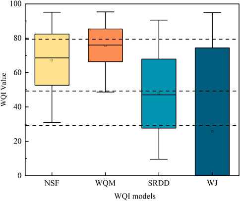
FIGURE 3. WQI values computed by four different WQI models. Horizontal dashed lines indicate the values used to classify the groundwater quality (see Table 2). Hollow squares indicate the mean values, and solid black lines in each box indicate the median WQI values.

Figure 4 shows the groundwater quality classification results for WQI-BMA value distribution predicted using BMA. Groundwater quality status can be categorized into four types based on WQI values: poor (0–29), marginal (29–49), fair (50–79), and good (80–100) (Table 2). WQI-BMA values ranged from 35.01 to 98.45 based on BMA prediction. According to the groundwater quality classification of WQI values (Table 2), the groundwater quality status was classified into three categories: marginal, fair, and good. Based on the WQI-BMA model, 17.6% of the groundwater fell under the marginal category, 45.7% fell under the fair category, and 36.7% fell under the good groundwater quality category.

FIGURE 4

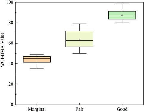
FIGURE 4. WQI-BMA values after groundwater quality classification predicted by BMA. Hollow squares indicate the mean values, and solid black lines in each box indicate the median WQI-BMA values.

3.4 Spatiotemporal distribution of groundwater quality

Figure 5 shows the percentages of groundwater quality classification in the study site over the dry and wet seasons from 2015 to 2020. Percentage of groundwater quality classification refers to the percentage of wells classified as marginal, fair, or good. During the period 2015–2020, the fairness category had the highest percentage of all categories, ranging from 43.3% to 83%, with an annual average of 54.7%. In contrast, the marginal category had the lowest percentage, ranging from 3.3% to 40%, with an annual average of 16.7%. The percentage of good categories was between fair and marginal, ranging from 13.3% to 43.3%, with an annual average of 28.6%. Regarding seasonal variation, there were differences in the groundwater quality status over the dry and wet seasons during the study period (2015–2020). For example, the seasonal variation in the groundwater quality in the fair category was small, ≤7%, except in 2015. However, groundwater quality in the marginal and good categories varied the most in 2020 at 20% and 13%, respectively.

FIGURE 5

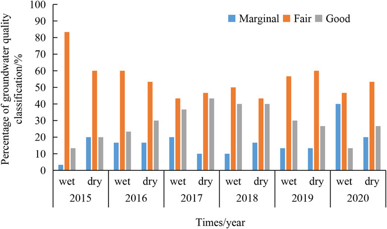
FIGURE 5. Percentage of groundwater quality classification over dry and wet seasons from 2015 to 2020. Percentage of groundwater quality classification indicates the percentage of wells classified as marginal, fair, or good in terms of water quality.

Geographic information system-based spatiotemporal analysis was used to determine the spatiotemporal distribution of the WQI map in the study area from 2015 to 2020 (Figure 6). Spatially, most sites fell under the fair-to-good category, with a few scattered areas falling under the marginal category, indicating that groundwater quality of the study area has been well maintained over the past few years. Specifically, the best areas for groundwater quality classification are the eastern parts of the city, such as Dapeng and Yantian. This area is mostly mountainous and hilly, with abundant forest resources. Due to the lack of heavy industry, the maintenance of groundwater quality is better. There are a total of 12 monitoring wells in the region. In 2015, there were two wells fell under the good category, nine wells fell under the fair category, and one well fell under the marginal category. With the development of smart water management, groundwater quality has gradually improved by 2019. There were seven wells fell under the good category, four wells fell under the fair category, and one well fell under the marginal category. The western region of the study area is an industrial agglomeration, the central part is the city center area with dense population, and the quality of groundwater is worse than that of the eastern region. Subsequent monitoring of groundwater quality should be strengthened in the central and western regions, especially in the coastal areas of the west. None of the samples in the study area fell under the poor and inappropriate for drinking categories. These results indicate that during the scarcity of surface water, groundwater can be used as a recharge source. Overall, the spatial distribution of groundwater quality in the study area showed that most of the groundwater in the study area was above the fair category and suitable for most applications.

FIGURE 6

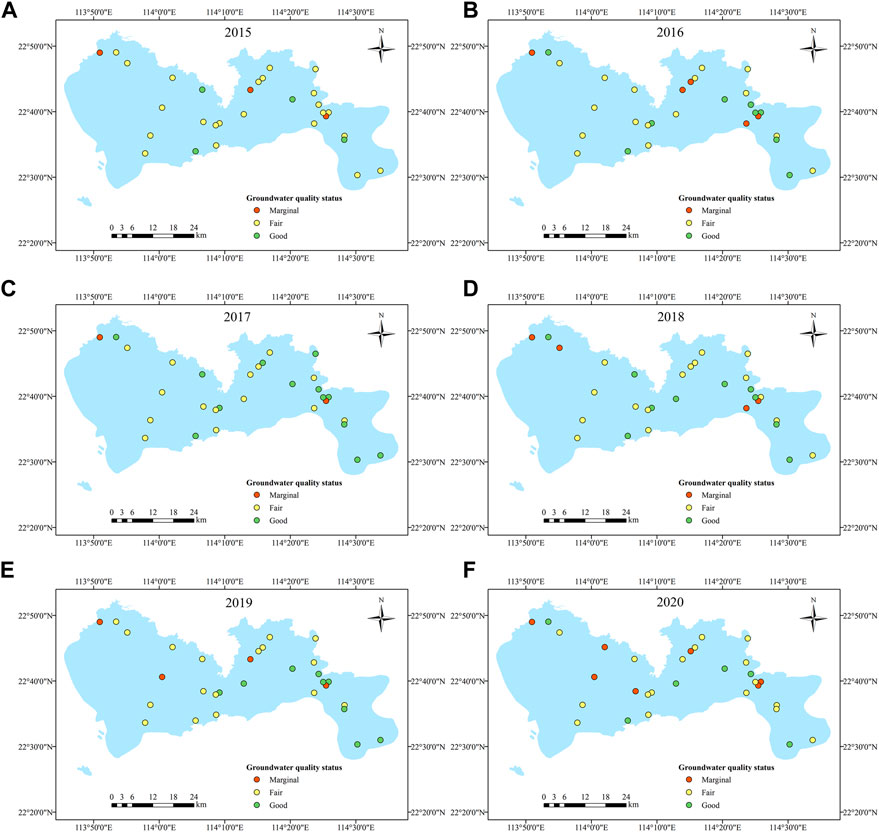
FIGURE 6. Spatiotemporal distribution of the groundwater quality status in the study area from 2015 to 2020.

Temporally, the groundwater quality in the study area showed seasonal fluctuations from 2015 to 2020. Relatively, the number of wells in the marginal groundwater quality category first increased, then decreased, and subsequently increased over time. Notably, 2020 had the highest number of sites in the marginal category. The number of wells in the good groundwater quality category first increased and then stabilized, followed by a decrease over time. The number of wells in the good groundwater quality category increased significantly compared to those in 2015. In contrast, the fair groundwater quality category remained at a relatively stable level. Overall classification of groundwater in the study area was mainly above the marginal category and suitable for domestic and agricultural use. Basic data for the model input were groundwater monitoring data. For emerging pollutants, the monitoring data of the relevant pollutants can be collected and introduced into the model for evaluation; however, currently, there is no threshold standard for the limit value of emerging pollutants in groundwater. Therefore, threshold standards need to be determined in the future along with relevant toxicological studies.

4 Conclusion

In this study, a WQI-BMA model was developed by combining the BMA and WQI methods to assess the groundwater quality status. The developed model could quantify model uncertainty and reasonably assess the groundwater quality status. As this model uses an approach combining the XGboost and ROC weight methods, it provides better results than other models using the expert opinion method. Sub-index calculation in this model is based on a uniform calculation rule to reduce model uncertainty owing to differences in the sub-index functions. We used the BMA method to quantify the uncertainty caused by four different WQI models. WQI-BMA model is a generic model that can be used to assess the groundwater quality in regions where the groundwater monitoring data are available.

In this study, the groundwater in Shenzhen was assessed to demonstrate the application and reliability of the proposed WQI-BMA model. Groundwater quality data from 2015 to 2021 were used to assess the groundwater quality and determine its spatiotemporal distribution. WQI values ranged from 35.01 to 98.45 based on the BMA prediction in the study area. The groundwater quality status could be classified into three categories: marginal, fair, and good. No water sample in the study area was categorized as poor or inappropriate for drinking. Most sites fell into the fair-to-good category. Temporally, the groundwater quality in the study area showed seasonal fluctuations from 2015 to 2020. Moreover, the highest percentage of seasonal variations was in the fair category. WQI-BMA model developed in this study can assess the suitability of groundwater sources and quantify uncertainty by incorporating the BMA method to provide a reliable assessment. It also provides a decision-support tool to aid decision-makers in groundwater quality management.

Data availability statement

The datasets presented in this article are not readily available because Data are not publicly available. Requests to access the datasets should be directed to 11849583@mail.sustech.edu.cn.

Author contributions

XW: Conceptualization, methodology, investigation, software, formal analysis, visualization, writing—original draft. YT: Methodology, software, supervision, writing—review and editing. CL: Conceptualization, writing—review and editing, Funding acquisition.

Funding

This work was supported by National key research and development program (project No. 2019YFC1803903).

Acknowledgments

The authors would like to thank the helpful discussion from Gang Tang, Rong Li, and Jiang Yu.

Conflict of interest

The authors declare that the research was conducted in the absence of any commercial or financial relationships that could be construed as a potential conflict of interest.

Publisher’s note

All claims expressed in this article are solely those of the authors and do not necessarily represent those of their affiliated organizations, or those of the publisher, the editors and the reviewers. Any product that may be evaluated in this article, or claim that may be made by its manufacturer, is not guaranteed or endorsed by the publisher.

Supplementary material

The Supplementary Material for this article can be found online at: https://www.frontiersin.org/articles/10.3389/fenvs.2023.1086300/full#supplementary-material

References

Abbaszadeh, M., Soltani-Mohammadi, S., and Ahmed, A. N. (2022). Optimization of support vector machine parameters in modeling of Iju deposit mineralization and alteration zones using particle swarm optimization algorithm and grid search method. Comput. Geosci. 165, 105140. doi:10.1016/j.cageo.2022.105140

CrossRef Full Text | Google Scholar

Abdelaziz, S., Gad, M. I., and El Tahan, A. H. M. H. (2020). Groundwater quality index based on PCA: Wadi El-Natrun, Egypt. J. Afr. Earth Sci. 172, 103964. doi:10.1016/j.jafrearsci.2020.103964

CrossRef Full Text | Google Scholar

Asadollah, S. B. H. S., Sharafati, A., Motta, D., and Yaseen, Z. M. (2021). River water quality index prediction and uncertainty analysis: A comparative study of machine learning models. J. Environ. Chem. Eng. 9 (1), 104599. doi:10.1016/j.jece.2020.104599

CrossRef Full Text | Google Scholar

Ashofteh, A., Bravo, J. M., and Ayuso, M. (2022). An ensemble learning strategy for panel time series forecasting of excess mortality during the COVID-19 pandemic. Appl. Soft. Comput. 128, 109422.

PubMed Abstract | CrossRef Full Text | Google Scholar

Bilgin, A. (2018). Evaluation of surface water quality by using Canadian council of ministers of the environment water quality index (CCME WQI) method and discriminant analysis method: A case study coruh river basin. Environ. Monit. Assess. 190 (9), 554. doi:10.1007/s10661-018-6927-5

PubMed Abstract | CrossRef Full Text | Google Scholar

Bordalo, A. A., Nilsumranchit, W., and Chalermwat, K. (2001). Water quality and uses of the bangpakong river (eastern Thailand). Water Res. 35 (15), 3635–3642. doi:10.1016/s0043-1354(01)00079-3

PubMed Abstract | CrossRef Full Text | Google Scholar

Bordalo, A. A., Teixeira, R., and Wiebe, W. J. (2006). A water quality index applied to an international shared river basin: The case of the douro river. Environ. Manage. 38 (6), 910–920. doi:10.1007/s00267-004-0037-6

PubMed Abstract | CrossRef Full Text | Google Scholar

Carvalho, L., Cortes, R., and Bordalo, A. A. (2011). Evaluation of the ecological status of an impaired watershed by using a multi-index approach. Environ. Monit. Assess. 174 (1-4), 493–508. doi:10.1007/s10661-010-1473-9

PubMed Abstract | CrossRef Full Text | Google Scholar

Chen, Y., Yuan, H. L., Yang, Y. Z., and Sun, R. C. (2020). Sub-daily soil moisture estimate using dynamic Bayesian model averaging. J. Hydrol. 590, 125445. doi:10.1016/j.jhydrol.2020.125445

CrossRef Full Text | Google Scholar

Duan, Q. Y., Ajami, N. K., Gao, X. G., and Sorooshian, S. (2007). Multi-model ensemble hydrologic prediction using Bayesian model averaging. Adv. Water Resour. 30 (5), 1371–1386. doi:10.1016/j.advwatres.2006.11.014

CrossRef Full Text | Google Scholar

Elbeltagi, A., Pande, C. B., Kouadri, S., and Islam, A. M. T. (2022). Applications of various data-driven models for the prediction of groundwater quality index in the Akot basin, Maharashtra, India. Environ. Sci. Pollut. Res. 29 (12), 17591–17605. doi:10.1007/s11356-021-17064-7

CrossRef Full Text | Google Scholar

Gharekhani, M., Nadiri, A. A., Khatibi, R., Sadeghfam, S., and Moghaddam, A. A. (2022). A study of uncertainties in groundwater vulnerability modelling using Bayesian model averaging (BMA). J. Environ. Manage. 303, 114168. doi:10.1016/j.jenvman.2021.114168

PubMed Abstract | CrossRef Full Text | Google Scholar

Gupta, S., and Gupta, S. K. (2021). A critical review on water quality index tool: Genesis, evolution and future directions. Ecol. Inf. 63, 101299. doi:10.1016/j.ecoinf.2021.101299

CrossRef Full Text | Google Scholar

Hoeting, J. A., Madigan, D., Raftery, A. E., and Volinsky, C. T. (1999). Bayesian model averaging: A tutorial. Stat. Sci. 14 (4), 382–401. doi:10.1214/ss/1009212519

CrossRef Full Text | Google Scholar

Ibn Ali, Z., Gharbi, A., and Zairi, M. (2020). Evaluation of groundwater quality in intensive irrigated zone of Northeastern Tunisia. Groundw. Sustain. Dev. 11, 100482. doi:10.1016/j.gsd.2020.100482

CrossRef Full Text | Google Scholar

Juwana, I., Muttil, N., and Perera, B. J. C. (2016). Uncertainty and sensitivity analysis of West Java water sustainability index - a case study on citarum catchment in Indonesia. Ecol. Indic. 61, 170–178. doi:10.1016/j.ecolind.2015.08.034

CrossRef Full Text | Google Scholar

Lap, B. Q., Phan, T.-T.-H., Nguyen, H. D., Quang, L. X., Hang, P. T., Phi, N. Q., et al. (2023). Predicting water quality index (WQI) by feature selection and machine learning: A case study of an kim hai irrigation system. Ecol. Inf. 74, 101991. doi:10.1016/j.ecoinf.2023.101991

CrossRef Full Text | Google Scholar

Li, J. T., An, X. Q., Li, Q. Y., Wang, C., Yu, H. M., Zhou, X. Y., et al. (2022). Application of XGBoost algorithm in the optimization of pollutant concentration. Atmos. Res. 276, 106238. doi:10.1016/j.atmosres.2022.106238

CrossRef Full Text | Google Scholar

Li, P. Y., and Wu, J. H. (2019). Drinking water quality and public health. Expos. Health. 11 (2), 73–79. doi:10.1007/s12403-019-00299-8

CrossRef Full Text | Google Scholar

Li, Z. Q. (2022). Extracting spatial effects from machine learning model using local interpretation method: An example of SHAP and XGBoost. Comput. Environ. Urban Syst. 96, 101845. doi:10.1016/j.compenvurbsys.2022.101845

CrossRef Full Text | Google Scholar

Lowe, L., Szemis, J., and Webb, J. A. (2017). “Uncertainty and environmental water,” in Water for the environment (Cambridge: Academic Press), 317–344. doi:10.1016/B978-0-12-803907-6.00015-2

CrossRef Full Text | Google Scholar

Lumb, A., Sharma, T. C., and Bibeault, J. F. (2011). A review of genesis and evolution of water quality index (WQI) and some future directions. Water Qual. Expo. Health. 3 (1), 11–24. doi:10.1007/s12403-011-0040-0

CrossRef Full Text | Google Scholar

Ma, Z., Li, H. X., Ye, Z. Y., Wen, J. P., Hu, Y., and Liu, Y. (2020). Application of modified water quality index (WQI) in the assessment of coastal water quality in main aquaculture areas of Dalian, China. Mar. Pollut. Bull. 157, 111285. doi:10.1016/j.marpolbul.2020.111285

PubMed Abstract | CrossRef Full Text | Google Scholar

Naghibi, S. A., Hashemi, H., Berndtsson, R., and Lee, S. (2020). Application of extreme gradient boosting and parallel random forest algorithms for assessing groundwater spring potential using DEM-derived factors. J. Hydrol. 589, 125197. doi:10.1016/j.jhydrol.2020.125197

CrossRef Full Text | Google Scholar

Nong, X. Z., Shao, D. G., Zhong, H., and Liang, J. K. (2020). Evaluation of water quality in the South-to-North Water Diversion Project of China using the water quality index (WQI) method. Water Res. 178, 115781. doi:10.1016/j.watres.2020.115781

PubMed Abstract | CrossRef Full Text | Google Scholar

Pan, B. Z., Han, X., Chen, Y., Wang, L. X., and Zheng, X. (2022). Determination of key parameters in water quality monitoring of the most sediment-laden Yellow River based on water quality index. Process Saf. Environ. Prot. 164, 249–259. doi:10.1016/j.psep.2022.05.067

CrossRef Full Text | Google Scholar

Qiu, G. Y., Zou, Z. D., Li, W. J., Li, L. J., and Yan, C. H. (2022). A quantitative study on the water-related energy use in the urban water system of Shenzhen. Sustain. Cities Soc. 80, 103786. doi:10.1016/j.scs.2022.103786

CrossRef Full Text | Google Scholar

Roszkowska, E. (2013). Rank ordering criteria weighting methods-a comparative overview. Optimum. Stud. Ekon. 5, 14–33. doi:10.15290/ose.2013.05.65.02

CrossRef Full Text | Google Scholar

Smith, D. G. (1990). A better water-quality indexing system for rivers and streams. Water Res. 24 (10), 1237–1244. doi:10.1016/0043-1354(90)90047-a

CrossRef Full Text | Google Scholar

Sutadian, A. D., Muttil, N., Yilmaz, A. G., and Perera, B. J. C. (2018). Development of a water quality index for rivers in West Java Province, Indonesia. Ecol. Indic. 85, 966–982. doi:10.1016/j.ecolind.2017.11.049

CrossRef Full Text | Google Scholar

Sutadian, A. D., Muttil, N., Yilmaz, A. G., and Perera, B. J. C. (2015). Development of river water quality indices-a review. Environ. Monit. Assess. 188 (1), 58. doi:10.1007/s10661-015-5050-0

PubMed Abstract | CrossRef Full Text | Google Scholar

Sutadian, A. D., Muttil, N., Yilmaz, A. G., and Perera, B. J. C. (2017). Using the Analytic Hierarchy Process to identify parameter weights for developing a water quality index. Ecol. Indic. 75, 220–233. doi:10.1016/j.ecolind.2016.12.043

CrossRef Full Text | Google Scholar

Tomas, D., Curlin, M., and Maric, A. S. (2017). Assessing the surface water status in Pannonian ecoregion by the water quality index model. Ecol. Indic. 79, 182–190. doi:10.1016/j.ecolind.2017.04.033

CrossRef Full Text | Google Scholar

Uddin, M. G., Nash, S., and Olbert, A. I. (2021). A review of water quality index models and their use for assessing surface water quality. Ecol. Indic. 122, 107218. doi:10.1016/j.ecolind.2020.107218

CrossRef Full Text | Google Scholar

Uddin, M. G., Nash, S., Rahman, A., and Olbert, A. I. (2022). A comprehensive method for improvement of water quality index (WQI) models for coastal water quality assessment. Water Res. 219, 118532. doi:10.1016/j.watres.2022.118532

PubMed Abstract | CrossRef Full Text | Google Scholar

United Nations (2022). The united nation World water development report 2022: Groundwater: Making the invisible visible. Paris: UNESCO.

Google Scholar

Wang, D., Thunell, S., Lindberg, U., Jiang, L. L., Trygg, J., and Tysklind, M. (2022a). Towards better process management in wastewater treatment plants: Process analytics based on SHAP values for tree-based machine learning methods. J. Environ. Manage. 301, 113941. doi:10.1016/j.jenvman.2021.113941

PubMed Abstract | CrossRef Full Text | Google Scholar

Wang, J., Bao, W. M., Xiao, Z. L., and Si, W. (2022b). Multi-model integrated error correction for streamflow simulation based on Bayesian model averaging and dynamic system response curve. J. Hydrol. 607, 127518. doi:10.1016/j.jhydrol.2022.127518

CrossRef Full Text | Google Scholar

Wu, T., Wang, S. R., Su, B. L., Wu, H. X., and Wang, G. Q. (2021). Understanding the water quality change of the Yilong Lake based on comprehensive assessment methods. Ecol. Indic. 126, 107714. doi:10.1016/j.ecolind.2021.107714

CrossRef Full Text | Google Scholar

Wu, Z. S., Wang, X. L., Chen, Y. W., Cai, Y. J., and Deng, J. C. (2018). Assessing river water quality using water quality index in Lake Taihu Basin, China. Sci. Total Environ. 612, 914–922. doi:10.1016/j.scitotenv.2017.08.293

PubMed Abstract | CrossRef Full Text | Google Scholar

Yumnam, K., Guntu, R. K., Rathinasamy, M., and Agarwal, A. (2022). Quantile-based Bayesian Model Averaging approach towards merging of precipitation products. J. Hydrol. 604, 127206. doi:10.1016/j.jhydrol.2021.127206

CrossRef Full Text | Google Scholar

Zhu, M., Wang, J., Yang, X., Zhang, Y., Zhang, L., Ren, H., et al. (2022). A review of the application of machine learning in water quality evaluation. Eco-Environment Health 1 (2), 107–116. doi:10.1016/j.eehl.2022.06.001

CrossRef Full Text | Google Scholar