Regimentation of geochemical indicator elements employing convolutional deep learning algorithm

Recently, deep learning algorithms have been popularly developed for identifying multi-element geochemical patterns related to various mineralization occurrences. Effective recognition of multi-element geochemical anomalies is essential for mineral exploration, and effective recognition is extremely dependent on integral clustering. Deep learning algorithms can achieve impressive results in comparison to the prior methods of clustering indicator elements correlated to mineralization for a region of interest due to their superb capability of extracting features from complex data. Although numerous supervised and unsupervised deep learning algorithms have been executed for the recognition of geochemical anomalies, employing them for clustering geochemical indicator elements is rarely observed. In this research, a convolutional deep learning (CDL) algorithm was architected to recognize and regiment geochemical indicator elements in Takht-e Soleyman District, Iran. Various opinions and experiments were considered to reach optimum parameters of this architecture. Fortunately, the achieved root mean square error (RMSE) values were in the appropriate range (<20%) which display the predicted values of the dependent variables (Pb as a pioneer of the first group and Ag as a pioneer of the second group) through their independent variables that are so close to their actual values. Also, the great R²adj calculated (more than 90%) for the last stage of regimentation confirms impressive accuracy and performance of the convolutional deep learning algorithm for clustering geochemical indicator elements of the study area.

1 Introduction

Appropriate regimentation of geochemical indicator elements of mineralization occurrences is a challenging issue due to the complexity of geological features, especially for a big geochemical data collection of stream sediments on a regional scale (Ghezelbash et al., 2019; Ghezelbash et al., 2020). Dividing geochemical indicator elements associated with mineral deposits into efficient and inefficient groups can be different due to employing various traditional clustering methods or factor analysis techniques (Templ et al., 2008; Yang et al., 2016). Thus, employment of a suitable methodology such as convolutional deep learning (CDL) algorithm can regiment big geochemical data into meaningful groups of indicator elements. In fact, complexity and diversity of geological features and application of various clustering methods can influence numbers and types of indicator element groups and complicate geochemical anomaly detection. Therefore, clustering indicator elements analyzed into efficient groups is a fundamental operation in the initial stages of mineral exploration (Ghezelbash et al., 2020). Traditional clustering procedures such as fuzzy c-means, K-medoids, and K-means classified as unsupervised techniques are carried out for discriminating geochemical data into homogeneous groups or clusters for distinguishing background and anomaly populations (Clare and Cohen 2001) or alterations and lithological units (Yang et al., 2016), while machine learning algorithms and the CDL structure can especially be executed for professional regimentation of geochemical indicator elements. The big amount of geochemical data on stream sediments is commonly regarded as compositional data that display multivariate behavior (Ghezelbash et al., 2020). Hence, architecting a CDL structure that includes multivariate regression can be so effective. Previously, response surface regression, polynomial regression, factorial regression, and multiple regression were executed by many researchers (Howarth 2001; Coburn, Freeman et al., 2012; Granian, Tabatabaei et al., 2015; Sabbaghi 2018). Response surface regression has been widely applied in earth science fields due to its nature. In fact, the function achieved from response surface regression has been prevalently employed to present the behavior of a dependent variable with respect to independent variables to discover the optimum position of effective variables through particular parameters in environmental sciences. Convolutional neural networks (LeCun et al., 2015), deep belief nets (Hinton et al., 2006), artificial neural networks (Anderson 1972), logistic regression (Cox 1959), ensemble learning (Dietterich 2002), random forest (Breiman 2001), and support vector machine (Vapnik 1999) classified as supervised learning algorithms are concentrated on classifying situations, issues, or objects according to the known data labeled into a machine. Moreover, feature extraction (Coates et al., 2011; Sabbaghi and Moradzadeh 2018; Sabbaghi and Tabatabaei 2023), dimensional reduction (Redlich 1993), and density estimation (Scott and Knott 1974; Silverman 2018) classified as unsupervised learning algorithms are applied to detect hidden potential patterns of a big dataset without the known labeled data (Pal, Ruidas et al., 2022). The machine learning methods such as support vector machine and random forest are considered shallow learning methods and only include one hidden layer or can even be without hidden layers. Therefore, their development ability is generally restricted to distribution issues of big complex data. The observable difference between the aforementioned networks with a hidden layer and deep learning networks is epitomized in their depth (Chakrabortty, Pal et al., 2021; Ruidas, Pal et al., 2021; Roy et al., 2022; Saha et al., 2022). Thus, more complex features can be extracted through deep learning networks because high-level features are created by combining low-level features. A deep autoencoder network was initially applied to map mineralization zones of an iron polymetallic deposit by Xiong and Zuo (2016). Subsequently, deep learning networks became more popular in several fields of mineral exploration (Zuo 2017; Zuo 2020; Zhang et al., 2021). For example, the GoogLeNet, as a convolutional neural network, was employed to map potential zones of gold deposits by Yang, Zhang et al. (2021). However, disregarding domain knowledge and experiments in purely data-driven deep learning networks can frequently lead to interpretation trouble from the geochemical perspective. In conclusion, incorporating geochemical knowledge and expert’s opinions into deep learning networks can create new challenges in this field. This research intends to present an unsupervised CDL algorithm for clustering geochemical indicator elements of the Mississippi Valley-type (MVT) Pb–Zn deposit in Takht-e Soleyman District in Iran. We attached a regression layer to the constructed network and performed a known forward strategy of multivariate regression for predicting values of pioneer elements of each cluster.

2 Study area

2.1 Takht-e Soleyman zone

This area is considered a significant part of the Takab mineralization zone in West Azerbaijan Province, Iran. The Takht-e Soleyman region is restricted between 47° 0′ 0˝ E and 47° 30′ 0˝ E longitudes and 36° 30′ 0˝ N and 37° 0′ 0˝ N latitudes, which is exactly situated between the Urumieh–Dokhtar Volcanic Arc (UDVA) and the Sanandaj–Sirjan Zone (SSZ) (Figure 1). The extensional faults of the region commonly has an E–W or NE–SW trend, which is considered the mineralization factor for MVT Pb–Zn deposits and epithermal gold deposits. The geological structures of this zone mostly contain carbonated, metamorphic, and sedimentary rocks and volcanic outcrops that are rarely observed.

FIGURE 1

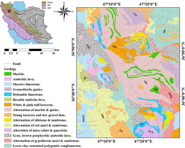
FIGURE 1. Simplified geological map (1:100,000) of the region of interest (Takht-e Soleyman).

2.2 MVT Pb–Zn mineralization

The MVT Pb–Zn deposits typically occur as stratiform in passive margin settings and have continuous and huge orebodies that are weakly associated with their alterations (dolomitization and silicification) (Wei et al., 2020). It is known that 25% of lead–zinc requirements of the world are supplied through the MVT Pb–Zn deposits. Therefore, they are remarkable in mineral prospectivity mapping (Sabbaghi and Tabatabaei 2020; Sabbaghi and Tabatabaei 2022). These deposits are hosted by carbonate rocks (dolostone and limestone), which are observed in foreland basins of orogenic belts (Wei et al., 2020). Their simple ore mineralogy primarily includes Fe sulfides, galena, and sphalerite (Hosseini-Dinani and Aftabi 2016).

3 Methods

3.1 Multivariate regression

The regression procedure was introduced as a statistical method for considering relationships between variables. For instance, a dependent variable (Y) can be delineated through the function of independent variables (x_i) given as follows:

$Y=\mathrm{f}\left(x_i\right)(1)$

When Y is a linear function of x_i, regression is commonly named linear. Otherwise, regression would be non-linear with a delineated non-linear function. Vugrinovich (1989), Saunders et al. (1991), and Karathanasis (1999) have adequately performed linear and non-linear regression for investigating the behavior of different geoscience variables. Accordingly, the multivariate regression function is expressed as follows:

$Y=a_0+a_1{x}_1+a_2{x}_2+\dots +\mathit{\varepsilon }(2)$

where a₀ and a_i (i = 1, 2, ..., n) are the constant factor and partial coefficients, respectively, and Ɛ represents the random error. The random error value reveals the deviation of Y values predicted from their actual values. Prior studies (Granian et al., 2015; Karbalaei Ramezanali et al., 2020) have suggested the measured variable p for each sample, when a dataset contains n samples. Therefore, Eq. 2 can be represented as follows:

$Y_i={\widehat{a}}_0+{\widehat{a}}_1{x}_{i1}+{\widehat{a}}_2{x}_{i2}+\dots +{\widehat{a}}_p{x}_{ip}+{\mathit{\varepsilon }}_i,i=\mathrm{1,2},\dots ,n(3)$

also, its matrix form is calculated as follows:

$\left[Y\right]=\left[X\right]\left[A\right]+\left[\mathit{\varepsilon }\right](4)$

$\left[Y\right]=\left[\begin{array}{c}{Y}_1\\ Y_2\\ ⋮\\ Y_n\end{array}\right];\left[A\right]=\left[\begin{array}{c}{â}_0\\ {â}_1\\ ⋮\\ {â}_n\end{array}\right];\left[X\right]=\left[\begin{array}{ccccc}1& x_{11}& x_{12}& \cdots & x_{1p}\\ 1& x_{21}& x_{22}& \cdots & x_{2p}\\ ⋮& ⋮& ⋮& ⋮& ⋮\\ 1& x_{n1}& x_{n2}& \cdots & x_{np}\end{array}\right];\left[\mathit{\varepsilon }\right]=\left[\begin{array}{c}{\mathit{\varepsilon }}_1\\ {\mathit{\varepsilon }}_2\\ ⋮\\ {\mathit{\varepsilon }}_n\end{array}\right](5)$

Regression coefficients are estimated by applying the least squares method expressed as follows:

$\left[A\right]={\left[Ʃ\right]}^{-1}\left[G\right]={\left({\left[X\right]}^{\prime }\left[X\right]\right)}^{-1}{\left[X\right]}^{\prime }\left[Y\right](6)$

where [G] is the covariance matrix between the independent variable and samples, [Ʃ]^-1 is the inverse of the variance–covariance matrix of the samples, and [A] is the coefficient matrix. For accepting the function fitted in regression analysis, the following three criterions should be prepared: 1) the variance and mean of the random error (ɛ) should be equal to the constant value and zero, respectively; 2) variance analysis should be performed until the function fitted into the data is significant (significance level α = 0.05, can be considered); and 3) calculating the determination coefficient (R²) using the following equation:

$R^2=\frac{{{\displaystyle \sum }}_{i=1}^n{\left({\mathrm{Ŷ}}_i-{Ȳ}_i\right)}^2}{{{\displaystyle \sum }}_{i=1}^n{\left(Y_i-{Ȳ}_i\right)}^2}=1-\frac{{{\displaystyle \sum }}_{i=1}^n{\left({\mathrm{Y}}_i-{\mathrm{Ŷ}}_i\right)}^2}{{{\displaystyle \sum }}_{i=1}^n{\left(Y_i-{Ȳ}_i\right)}^2}(7)$

where Ŷ_i, Ȳ_i, and Y_i are considered the estimated value of the ith dependent variable, mean of the dependent variable, and the ith dependent variable, respectively. While predicted values for the dependent variable (Ŷ_i) are close to their actual values (Y_i), it means that the regression model has been properly fitted and the determination coefficient (R²) is close to 1. Under the same condition, models have a higher priority while including a lower degree of complexity. The determination coefficient may be an appropriate parameter for considering multivariate regression models with the same number of independent variables, but it is not suitable for the comparison of models with various numbers of independent variables (Granian et al., 2015). Accordingly, the adjusted determination coefficient (R²adj) should be calculated as follows:

$R_{adj}^2=1-\frac{n-1}{n-t}\left(1-R^2\right)(8)$

where n and t are the number of samples and variables, respectively.

3.2 Convolutional neural network

A convolutional neural network (CNN) (Figure 2) regularly includes a convolutional layer, pooling layers, and fully connected layers that is recognized as a feedforward neural network (LeCun et al., 2015). The CNN was first executed for anomaly recognition and image classification in remote sensing data. A significant section of the CNN is the convolutional layer, which extracts high-level features of big datasets by using a convolutional procedure. Several advantages of a convolutional layer are as follows: 1) applying the weight sharing procedure for reducing parameters of a model and 2) maintaining invariance of an object location. The common two-dimensional convolution formula has been expressed by the following equation:

$G^{*}(X,Y)={\displaystyle \sum }_{i=1}^m{\displaystyle \sum }_{j=1}^{n}f(i‚j)·G\left(x-i+c‚y-j+c\right)(9)$

where f (x, y) plays the role of a filter for the convolving matrix G with n × m dimensions, resulting in the central result G*(x, y) around the central coordinate c. Convolutional layers are learned through some filters such as f which are generally followed by the application of the operation of a down-sampling in m and n for condensing spatial information. These forcing functions commonly aid in learning complicated representations in next convolutional layers progressively (Figure 2A). Pooling layers generally interfere along convolutional layers in a CNN for decreasing dimensions of network parameters and output features. Pooling layers are similar to convolutional layers because of considering neighboring features and can maintain translation invariant. The most applicable pooling operations are generally average pooling and max pooling. For example, a max pooling layer can reduce an 8 × 8 feature tensor to a 4 × 4 feature tensor through employing a window with 2 × 2 dimensions and a two-stride size (Figure 2B). The last layers of the CNN are commonly the fully connected layers, which are applied for classification and feature union (Figure 2C) (Krizhevsky et al., 2017). In fact, flattening output features into a column vector and subsequently converting them into a specific division for classification are the most significant duty of a fully connected layer (Guo et al., 2016).

FIGURE 2

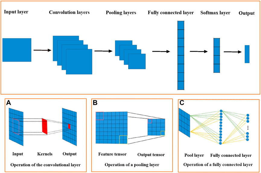
FIGURE 2. Common CNN framework.

3.3 Deep learning algorithm

Deep learning algorithms are a subset of machine learning algorithms which are employed to minimize the contrastive divergence of deep networks (comprising more processing layers) by applying an iterative training procedure. These algorithms generally encode training samples and rebuild them when they are consecutively represented to the network. Accordingly, interlayer connection weights are being continuously moderated. In machine learning algorithms, suitable iterations can only create a well-trained model for converging into a general solution. For machine learning algorithms, a necessary number of iterations are only revealed using the trial-and-error procedure, while deep learning algorithms can present a number of suitable iterations with the least value of loss through loss function, which has been embedded in their structures. The requirement data for deep learning algorithms were typically divided into training, testing, and validation data. Training data are applied for the descending gradient procedure on the objective function. In the training procedure, the model result is tested through testing data (unseen data). Validation data are ultimately applied to evaluate network performance.

3.4 Data preparation

A total of 868 stream sediment samples were collected from the region of interest. The collected samples were analyzed to consider 38 elements by the induced coupled plasma method. For each 20 measurements, the duplicated sub-samples were analyzed for considering the precision of the analyzing procedure. The analyzing error was less than ±10%. The stream sediment data are generally compositional data that are concerned with the problem of data closure. Accordingly, moderating outlier values were calculated by applying the robust Mahalanobis distance procedure. Then, stream sediment data were preprocessed by applying the isometric log-ratio transformation for removing the data closure problem and transforming into the range of [0, 1] (Wang et al., 2014).

4 Results and discussion

The CDL framework generally requires training, validation, and testing data. Hence, the 868 collected samples were prevalently divided as follows: 80% training data (608 samples), 10% validation data (87 samples), and 20% test data (173 samples). The CDL parameters (such as learning rate and minimum batch size) and the number of network layers were regulated through the trial-and-error procedure for extracting high-level features of multivariate geochemical data. The speed of back propagation as the performance of the training procedure is generally determined by the learning rate factor. Empirical studies displayed that for conducting the best training, the learning rate factor should be 0.01. We architected a CDL network employing the convolutional layer for clustering geochemical indicator elements with the learning rate of 0.01, learning rate drop factor of 0.7, learning rate drop period of 50, validation frequency of 50, maximum epoch of 30, and minimum batch size of 16. Also, we employed a kernel window with 2 × 2 dimensions and a one-stride size for the convolutional layer. Prior studies established an essential role of indicator elements such Pb, Zn, Ag, As, Cd, and Sb in the detection of primary and secondary dispersion halos of the MVT deposit (Wang et al., 2017; Li et al., 2018; Williams et al., 2020). As the first step of regimentation, we choose Pb and Ag elements as pioneers of the first and second groups, respectively. Based on Pearson’s correlation coefficients (Table 1), Pb presented a high correlation to the Zn element, while Ag exhibited a great correlation to Cd, As, and Sb. In this research, a forward strategy of multivariate regression was applied for clustering geochemical indicator elements by training a CDL network. Figure 3A clears the difference between actual values of Pb (as a dependent variable) and its predicted values through Zn values (as an independent variable) for the seventh training of the network. It is clear that the dependent variable (Pb) has been properly predicted via the correlated independent variable (Zn). The great adjusted determination coefficient (R²adj) of this process (up to 0.9) establishes this claim (Table 2). Furthermore, the seventh testing procedure was concurrently performed to consider the aforementioned difference in the test data, which have been assumed as unseen data (Figure 3B). The R²adj of the testing data is also exhibited in Table 2. In fact, the seventh training of the dataset has reached the best training performance with the least training loss which has decreased to 0.1 (Figure 4). Furthermore, the root mean square error (RMSE), which is commonly employed to evaluate predicted values of the dependent variable, has been presented as a diagram in Figure 4. This parameter clears that the estimation of Pb values through Zn values is an ideal condition (less than 0.2). So the first group that is regimented can play an essential role in detecting mineralization zones. The regimentation of the second group assumes the Cd element as its second member. The predicted values of Ag via Cd values display minor errors in their actual values (Figure 5A). Although, the R²adj calculated for training data (equal to 0.869) and testing data (equal to 0.852) highlights these minor errors (Table 2). In fact, the fifth training (Figure 5A) and testing (Figure 5B) of the network have achieved these results and have great conformity together. Also, the loss and RMSE values of the fifth training were depicted in Figure 6. Accordingly, it can be observed that the loss value has decreased up to 0.1 again and the RMSE is less than 0.2. The regimentation procedure is continued by selecting the As element as the third member of the second group. Figure 7A establishes that selecting As next as an independent variable for aiming the estimation of Ag values can smooth the prediction procedure because the achieved R²adj is more than the back stage. The forward strategy of multivariate regression claims that if adding an element into a group is associated with an impressive increment of the R²adj, the selected element will be a steady member, otherwise it should be eliminated (Granian et al., 2015). Therefore, the As element is the third permanent member of the second group because the R²adj calculated [training (0.889) and testing (0.878)] for this stage has impressive differences in the coefficients of the back stage (0.869 and 0.852). Also, choosing As as the third element of this group can be evaluated considering the test data condition (Figure 7B). Running the network for the fourth time created this progress, whose results have been presented in Figure 8. The loss value has similarly decreased close to 0.1 with the RMSE up to 0.2. Finally, the Sb element is imported as the fourth element into the second group. In addition to the proper estimation of Ag values via Sb values in training data (Figure 9A), testing data have achieved acceptable results (Figure 9B). Hence, Table 2 clearly shows impressive progress of the R²adj for both training (0.934) and testing data (0.926) again. This is a pleasant consequence, which maintains the Sb element in the second group. Furthermore, the loss value (up to 0.05) and the RMSE value (up to 0.15) (Figure 10) of the third training of the network can remunerate the regimentation procedure of the second group and terminate the clustering process. In fact, loss and RMSE values have sufficiently decreased and can validate the regimentation procedure.

TABLE 1

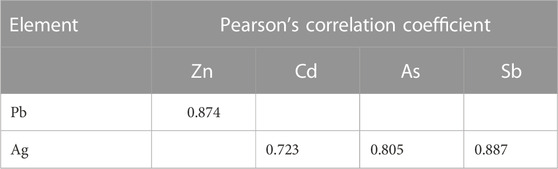
TABLE 1. Pearson’s correlation coefficients between significant geochemical indicator elements.

FIGURE 3

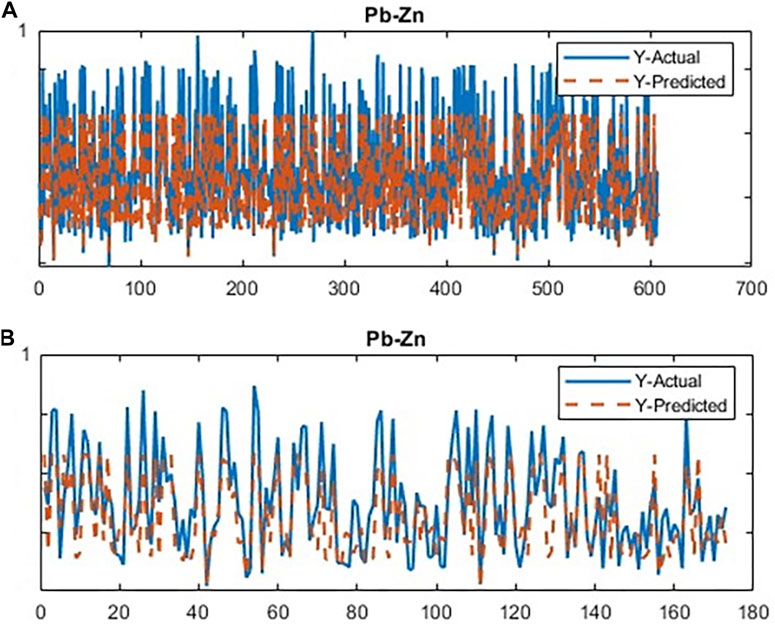
FIGURE 3. Plot of the running CDL network for clustering the first group of geochemical indicator elements (Pb–Zn); (A) training data and (B) testing data.

TABLE 2

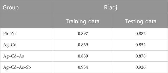
TABLE 2. Calculated R²adj of training and testing data for both groups of indicator elements in all stages.

FIGURE 4

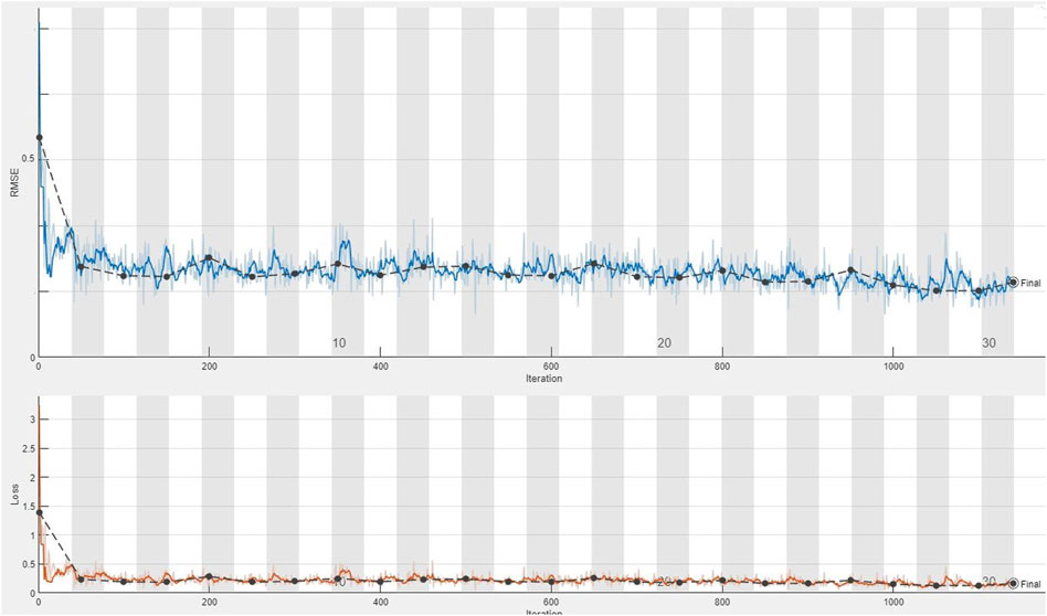
FIGURE 4. Plot of the seventh training of the dataset applying the CDL network for calculating the loss value and RMSE parameter from the first group of geochemical indicator elements (Pb–Zn).

FIGURE 5

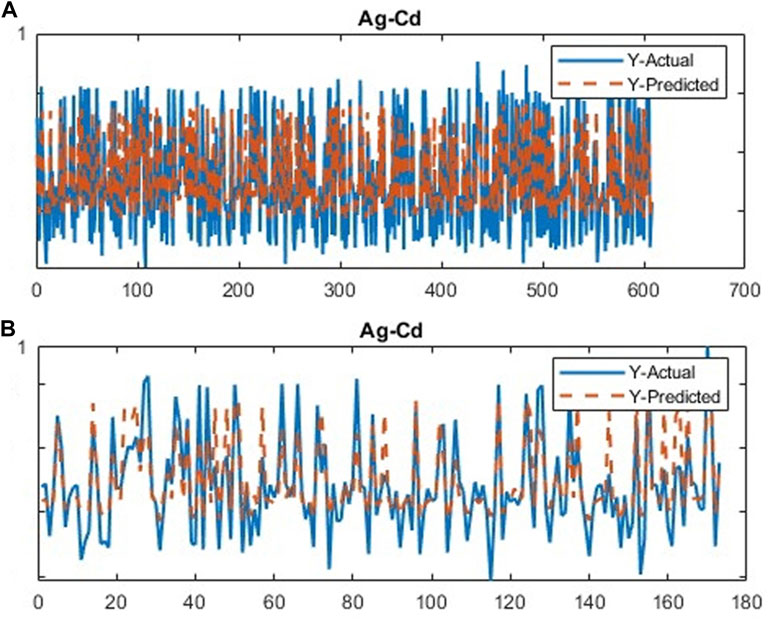
FIGURE 5. Plot of the running CDL network for the first stage of clustering the second group of geochemical indicator elements (Ag–Cd); (A) training data and (B) testing data.

FIGURE 6

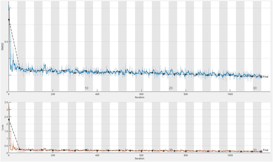
FIGURE 6. Plot of the fifth training of the dataset applying the CDL network for calculating the loss value and RMSE parameter from the second group of geochemical indicator elements (Ag–Cd).

FIGURE 7

FIGURE 7. Plot of the running CDL network for the second stage of clustering the second group of geochemical indicator elements (Ag–Cd–As); (A) training data and (B) testing data.

FIGURE 8

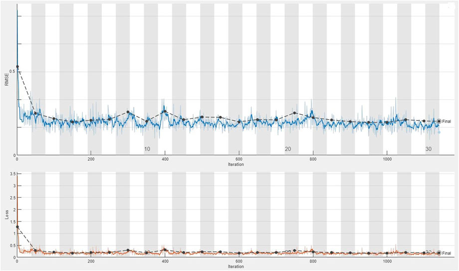
FIGURE 8. Plot of the fourth training of the dataset applying the CDL network for calculating the loss value and RMSE parameter from the second stage regimentation of the second group (Ag–Cd–As).

FIGURE 9

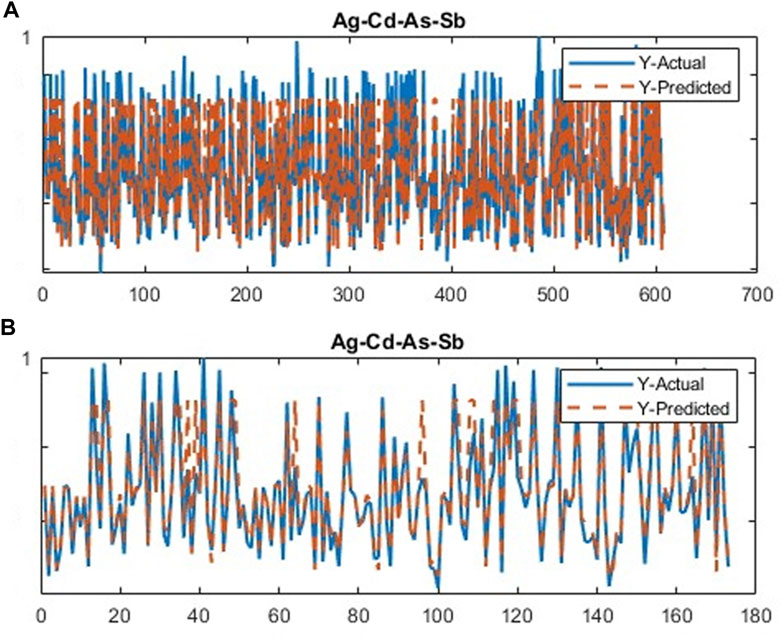
FIGURE 9. Plot of the running CDL network for the third stage of clustering the second group of geochemical indicator elements (Ag–Cd–As–Sb); (A) training data and (B) testing data.

FIGURE 10

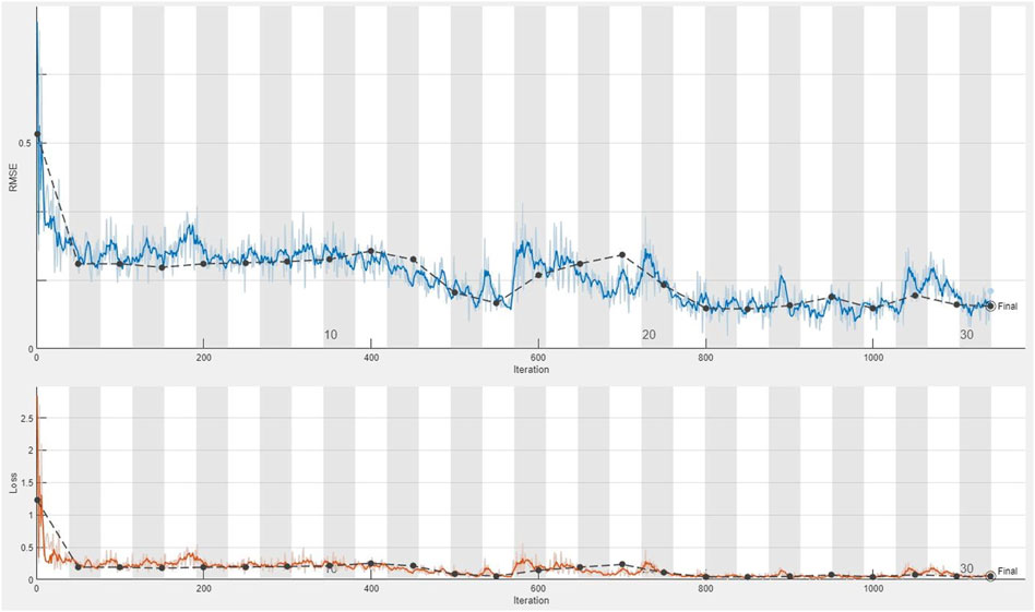
FIGURE 10. Plot of the third training of the dataset applying the CDL network for calculating the loss value and RMSE parameter from the third stage regimentation of the second group (Ag–Cd–As–Sb).

5 Conclusion

In this research, a hybrid procedure was created for multivariate regression, and a CDL algorithm was employed for clustering geochemical indicator elements of the MVT Pb–Zn deposit in the Takht-e Soleyman region, which is situated in West Azerbaijan Province, Iran. This hybrid network was architected to divide big geochemical data into training, validation, and testing samples randomly, and the utility and performance degree of the CDL were established using them. The results of this research exhibited that the CDL network with a multivariate regression layer can discriminate significant geochemical indicator elements related to a region of interest in appropriate clusters, while knowledge and experiments are incorporated into the network. The forward strategy of multivariate regression was performed for regimenting based on comparing the calculated R²adj after adding an indicator element into the group and before adding it. A CDL framework was constructed with optimum model parameters which regimented geochemical indicator elements into two groups: Pb and Zn as the first group and Ag, Cd, As, and Sb as the second group. For each stage of the training network, the R²adj of testing data was computed to evaluate the performance of the trained network, showing that all of them were in the acceptable range (more than 0.8). Furthermore, the loss function results of all acceptable trainings reached the least value expected (up to 0.1). Also, the RMSE value as a parameter for the validation of predicted values by the regression process can validate the training results by reaching the least value. Fortunately, the achieved RMSE values were in the appropriate range which display that predicted values of dependent variables (Pb as a pioneer of the first group and Ag as a pioneer of the second group) through their independent variables are so close to their actual values. Also, the great R²adj calculated (more than 90%) for the last stage of regimentation confirms impressive accuracy and performance of the CDL algorithm for clustering geochemical indicator elements of the study area. In fact, this study proposes a new approach for an unsupervised deep learning algorithm which includes the multivariate regression procedure for clustering or other targeting in other fields of geoscience.

Data availability statement

The original contributions presented in the study are included in the article/Supplementary Materials; further inquiries can be directed to the corresponding author.

Ethics statement

Written informed consent was obtained from the individual(s) for the publication of any potentially identifiable images or data included in this article.

Author contributions

ST was the supervisor for the research, and HS is the author of the paper.

Acknowledgments

The authors thank Aflak Exploration Company (SHS) for financial support of this manuscript. The funder was not involved in the study design, collection, analysis, interpretation of data, the writing of this article, or the decision to submit it for publication.

Conflict of interest

The authors declare that the research was conducted in the absence of any commercial or financial relationships that could be construed as a potential conflict of interest.

Publisher’s note

All claims expressed in this article are solely those of the authors and do not necessarily represent those of their affiliated organizations, or those of the publisher, the editors, and the reviewers. Any product that may be evaluated in this article, or claim that may be made by its manufacturer, is not guaranteed or endorsed by the publisher.

References

Anderson, J. A. (1972). A simple neural network generating an interactive memory. Math. Biosci. 14 (3-4), 197–220. doi:10.1016/0025-5564(72)90075-2

CrossRef Full Text | Google Scholar

Breiman, L. (2001). Random forests machine learning. Mach. Learn. 45, 5–32. View Article PubMed/NCBI Google Scholar. doi:10.1023/a:1010933404324

CrossRef Full Text | Google Scholar

Chakrabortty, R., Pal, S. C., Janizadeh, S., Santosh, M., Roy, P., Chowdhuri, I., et al. (2021). Impact of climate change on future flood susceptibility: An evaluation based on deep learning algorithms and GCM model. Water Resour. Manag. 35 (12), 4251–4274. doi:10.1007/s11269-021-02944-x

CrossRef Full Text | Google Scholar

Clare, A., and Cohen, D. (2001). A comparison of unsupervised neural networks and k-means clustering in the analysis of multi-element stream sediment data. Geochem. Explor. Environ. Anal. 1 (2), 119–134. doi:10.1144/geochem.1.2.119

CrossRef Full Text | Google Scholar

Coates, A., Ng, A., and Lee, H. (2011). “An analysis of single-layer networks in unsupervised feature learning,” in Proceedings of the fourteenth international conference on artificial intelligence and statistics, Fort Lauderdale, FL, USA, January 2011 (JMLR Workshop and Conference Proceedings), .

Google Scholar

Coburn, T. C., Freeman, P. A., and Attanasi, E. D. (2012). Empirical methods for detecting regional trends and other spatial expressions in Antrim Shale gas productivity, with implications for improving resource projections using local nonparametric estimation techniques. Nat. Resour. Res. 21 (1), 1–21. doi:10.1007/s11053-011-9165-x

CrossRef Full Text | Google Scholar

Cox, D. R. (1959). The regression analysis of binary sequences. J. R. Stat. Soc. Ser. B Methodol. 21 (1), 238–238. doi:10.1111/j.2517-6161.1959.tb00334.x

CrossRef Full Text | Google Scholar

Dietterich, T. (2002). Ensemble learning. The handbook of brain theory and neural networks. Arbib MA 2, 110–125.

Google Scholar

Ghezelbash, R., Maghsoudi, A., and Carranza, E. J. M. (2019). Mapping of single-and multi-element geochemical indicators based on catchment basin analysis: Application of fractal method and unsupervised clustering models. J. Geochem. Explor. 199, 90–104. doi:10.1016/j.gexplo.2019.01.017

CrossRef Full Text | Google Scholar

Ghezelbash, R., Maghsoudi, A., and Carranza, E. J. M. (2020). Optimization of geochemical anomaly detection using a novel genetic K-means clustering (GKMC) algorithm. Comput. Geosci. 134, 104335. doi:10.1016/j.cageo.2019.104335

CrossRef Full Text | Google Scholar

Granian, H., Tabatabaei, S. H., Asadi, H. H., and Carranza, E. J. M. (2015). Multivariate regression analysis of lithogeochemical data to model subsurface mineralization: A case study from the sari gunay epithermal gold deposit, NW Iran. J. Geochem. Explor. 148, 249–258. doi:10.1016/j.gexplo.2014.10.009

CrossRef Full Text | Google Scholar

Guo, Y., Liu, Y., Oerlemans, A., Lao, S., Wu, S., and Lew, M. S. (2016). Deep learning for visual understanding: A review. Neurocomputing 187, 27–48. doi:10.1016/j.neucom.2015.09.116

CrossRef Full Text | Google Scholar

Hinton, G. E., Osindero, S., and Teh, Y.-W. (2006). A fast learning algorithm for deep belief nets. Neural Comput. 18 (7), 1527–1554. doi:10.1162/neco.2006.18.7.1527

PubMed Abstract | CrossRef Full Text | Google Scholar

Hosseini-Dinani, H., and Aftabi, A. (2016). Vertical lithogeochemical halos and zoning vectors at Goushfil Zn–Pb deposit, Irankuh district, southwestern Isfahan, Iran: Implications for concealed ore exploration and genetic models. Ore Geol. Rev. 72, 1004–1021. doi:10.1016/j.oregeorev.2015.09.023

CrossRef Full Text | Google Scholar

Howarth, R. J. (2001). A history of regression and related model-fitting in the Earth sciences (1636?-2000). Nat. Resour. Res. 10 (4), 241–286. doi:10.1023/a:1013928826796

CrossRef Full Text | Google Scholar

Karathanasis, A. D. (1999). Subsurface migration of copper and zinc mediated by soil colloids. Soil Sci. Soc. Am. J. 63, 830–838.

CrossRef Full Text | Google Scholar

Karbalaei Ramezanali, A., Feizi, F., Jafarirad, A., and Lotfi, M. (2020). Geochemical anomaly and mineral prospectivity mapping for vein-type copper mineralization, kuhsiah-e-urmak area, Iran: Application of sequential Gaussian simulation and multivariate regression analysis. Nat. Resour. Res. 29 (1), 41–70. doi:10.1007/s11053-019-09565-7

CrossRef Full Text | Google Scholar

Krizhevsky, A., Sutskever, I., and Hinton, G. E. (2017). Imagenet classification with deep convolutional neural networks. Commun. ACM 60 (6), 84–90. doi:10.1145/3065386

CrossRef Full Text | Google Scholar

LeCun, Y., Bengio, Y., and Hinton, G. (2015). Deep learning. nature 521 (7553), 436–444. doi:10.1038/nature14539

PubMed Abstract | CrossRef Full Text | Google Scholar

Li, N., Xiao, K., Sun, L., Li, S., Zi, J., Wang, K., et al. (2018). Part I: A resource estimation based on mineral system modelling prospectivity approaches and analogical analysis: A case study of the MVT Pb-Zn deposits in huayuan district, China. Ore Geol. Rev. 101, 966–984. doi:10.1016/j.oregeorev.2018.02.014

CrossRef Full Text | Google Scholar

Pal, S. C., Ruidas, D., Saha, A., Islam, A. R. M. T., and Chowdhuri, I. (2022). Application of novel data-mining technique-based nitrate concentration susceptibility prediction approach for coastal aquifers in India. J. Clean. Prod. 346, 131205. doi:10.1016/j.jclepro.2022.131205

CrossRef Full Text | Google Scholar

Redlich, A. N. (1993). Redundancy reduction as a strategy for unsupervised learning. Neural Comput. 5 (2), 289–304. doi:10.1162/neco.1993.5.2.289

CrossRef Full Text | Google Scholar

Roy, P., Pal, S. C., Janizadeh, S., Chakrabortty, R., Islam, A. R. M. T., Chowdhuri, I., et al. (2022). Evaluation of climate change impacts on future gully erosion using deep learning and soft computational approaches. Geocarto Int. 29, 1–37. (just-accepted). doi:10.1080/10106049.2022.2071473

CrossRef Full Text | Google Scholar

Ruidas, D., Pal, S. C., Islam, A. R. M., and Saha, A. (2021). Characterization of groundwater potential zones in water-scarce hardrock regions using data driven model. Environ. Earth Sci. 80 (24), 809–818. doi:10.1007/s12665-021-10116-8

CrossRef Full Text | Google Scholar

Sabbaghi, H. (2018). A combinative technique to recognise and discriminate turquoise stone. Vib. Spectrosc. 99, 93–99. doi:10.1016/j.vibspec.2018.09.002

CrossRef Full Text | Google Scholar

Sabbaghi, H., and Moradzadeh, A. (2018). ASTER spectral analysis for host rock associated with porphyry copper-molybdenum mineralization. J. Geol. Soc. India 91 (5), 627–638. doi:10.1007/s12594-018-0914-x

CrossRef Full Text | Google Scholar

Sabbaghi, H., and Tabatabaei, S. H. (2020). A combinative knowledge-driven integration method for integrating geophysical layers with geological and geochemical datasets. J. Appl. Geophys. 172, 103915. doi:10.1016/j.jappgeo.2019.103915

CrossRef Full Text | Google Scholar

Sabbaghi, H., and Tabatabaei, S. H. (2022). Application of the most competent knowledge-driven integration method for deposit-scale studies. Arabian J. Geosci. 15 (11), 1057–1110. doi:10.1007/s12517-022-10217-z

CrossRef Full Text | Google Scholar

Sabbaghi, H., and Tabatabaei, S. H. (2023). Execution of an applicable hybrid integration procedure for mineral prospectivity mapping. Arabian J. Geosci. 16 (1), 3–13. doi:10.1007/s12517-022-11094-2

CrossRef Full Text | Google Scholar

Saha, A., Pal, S. C., Chowdhuri, I., Chakrabortty, R., and Roy, P. (2022). Understanding the scale effects of topographical variables on landslide susceptibility mapping in Sikkim Himalaya using deep learning approaches. Geocarto Int., 1–27. doi:10.1080/10106049.2022.2136255

CrossRef Full Text | Google Scholar

Saunders, D. F., Burson, K. R., and Thompson, C. K. (1991). Observed relation of soil magnetic susceptibility and soil gas hydrocarbon analyses to subsurface hydrocarbon accumulations. AAPG Bulletin 75, 389–408.

Google Scholar

Scott, A. J., and Knott, M. (1974). A cluster analysis method for grouping means in the analysis of variance. Biometrics 30, 507–512.

CrossRef Full Text | Google Scholar

Silverman, B. W. (2018). Density estimation for statistics and data analysis. Oxfordshire, England, UK: Routledge.

Google Scholar

Templ, M., Filzmoser, P., and Reimann, C. (2008). Cluster analysis applied to regional geochemical data: Problems and possibilities. Appl. Geochem. 23 (8), 2198–2213. doi:10.1016/j.apgeochem.2008.03.004

CrossRef Full Text | Google Scholar

Vapnik, V. (1999). The nature of statistical learning theory. Berlin, Germany: Springer science & business media.

Google Scholar

Vugrinovich, R. (1989). Subsurface temperatures and surface heat flow in the Michigan Basin and their relationships to regional subsurface fluid movement. Mar. Pet. Geol. 6, 60–70.

CrossRef Full Text | Google Scholar

Wang, K., Li, N., Bagas, L., Li, S., Song, X., and Cong, Y. (2017). GIS-based prospectivity-mapping based on geochemical multivariate analysis technology: A case study of MVT Pb–Zn deposits in the huanyuan-fenghuang district, northwestern hunan province, China. Ore Geol. Rev. 91, 1130–1146. doi:10.1016/j.oregeorev.2017.09.015

CrossRef Full Text | Google Scholar

Wang, W., Zhao, J., and Cheng, Q. (2014). Mapping of Fe mineralization-associated geochemical signatures using logratio transformed stream sediment geochemical data in eastern Tianshan, China. J. Geochem. Explor. 141, 6–14. doi:10.1016/j.gexplo.2013.11.008

CrossRef Full Text | Google Scholar

Wei, H., Xiao, K., Shao, Y., Kong, H., Zhang, S., Wang, K., et al. (2020). Modeling-based mineral system approach to prospectivity mapping of stratabound hydrothermal deposits: A case study of MVT Pb-Zn deposits in the huayuan area, northwestern hunan province, China. Ore Geol. Rev. 120, 103368. doi:10.1016/j.oregeorev.2020.103368

CrossRef Full Text | Google Scholar

Williams, N. D., Elliott, B. A., and Kyle, J. R. (2020). A predictive geospatial exploration model for Mississippi valley type Pb–Zn mineralization in the southeast Missouri lead district. Nat. Resour. Res. 29 (1), 285–310. doi:10.1007/s11053-020-09618-2

CrossRef Full Text | Google Scholar

Yang, H., Pan, H., Ma, H., Konaté, A. A., Yao, J., and Guo, B. (2016). Performance of the synergetic wavelet transform and modified K-means clustering in lithology classification using nuclear log. J. Petroleum Sci. Eng. 144, 1–9. doi:10.1016/j.petrol.2016.02.031

CrossRef Full Text | Google Scholar

Zhang, C., Zuo, R., and Xiong, Y. (2021). Detection of the multivariate geochemical anomalies associated with mineralization using a deep convolutional neural network and a pixel-pair feature method. Appl. Geochem. 130, 104994. doi:10.1016/j.apgeochem.2021.104994

CrossRef Full Text | Google Scholar

Zuo, R. (2020). Geodata science-based mineral prospectivity mapping: A review. Nat. Resour. Res. 29 (6), 3415–3424. doi:10.1007/s11053-020-09700-9

CrossRef Full Text | Google Scholar

Zuo, R. (2017). Machine learning of mineralization-related geochemical anomalies: A review of potential methods. Nat. Resour. Res. 26 (4), 457–464. doi:10.1007/s11053-017-9345-4

CrossRef Full Text | Google Scholar