The index of clothing for assessing tourism climate comfort: Development and application

Climate comfort is a significant factor in analyzing the effects of climate change on tourism, and considerable research has used multidimensional climate indices to evaluate climate comfort. In particular, the index of clothing (ICL) is recognized as one of the most popular climate indices and has been widely applied in many studies. While few studies focused on the calculation method of the index of clothing model’s surface solar radiation (R_act), the computed value was greater than that observed at ground stations. Thus, this study tried to improve solar radiation energy calculation on the Earth’s surface in the index of clothing model with the method recommended by the International Food and Agriculture Organization (FAO), and then validated the new model based on the meteorological data of 31 provincial capitals in mainland China during 1980–2019. Results showed that: 1) The value of R_act calculated by the International Food and Agriculture Organization (FAO) method was close to the site observations (P_bais < 15%), and was suggested to be used in enhancing the estimate approach for R_act in the index of clothing; 2) Different from the original index of clothing, ICL-new is significantly more effective in evaluating climate comfort in middle and low latitude regions; 3) Climate change had a considerable influence on the climate comfort of cities in mainland China. Since 1980, the climate comfort of cities in eastern China had increased in spring, while that of cities in western China had declined, and most cities had a decreasing trend in summer. Finally, our findings revealed that ICL-new can realistically and precisely depicts the actual scenario than the original index of clothing, and it is more suitable to provide scientific impact assessment and tourism management for government agencies and destination management.

Introduction

Climatic elements, as significant factors for the seasonal shifts in tourism (Feng et al., 2014; Scott et al., 2019), also affect the local tourism industry (Becken et al., 2020). Under the global warming scenario, climate change has posed significant challenges to international tourism development (Pintassilgo et al., 2016; Willibald et al., 2021), and some vulnerable areas worldwide have taken measures to deal with the consequences of climate change. Meanwhile, there is a growing focus on assessing climate comfort in tourism, geography, and meteorology (Liu et al., 2019; Loehr and Becken, 2021; Yu et al., 2021). Although the majority of studies have adopted multidimensional climate indices to evaluate tourism comfort in different regions (Dubois et al., 2016; Atzori et al., 2018; Zhong and Chen, 2019), there remains a lack of cases for their accuracy verification. Therefore, it is important to develop a scientific climate comfort model to assess climate comfort, which can be helpful to both tourism destination management and tourists’ travel decisions.

Climate comfort refers to the condition of comfort and suitability in which people experience normal physiological processes and feel comfortable without taking any additional thermal measures (Ma et al., 2009). This condition includes a comprehensive effect of external meteorological environment factors, such as the temperature, humidity, wind speed, and sunshine (Sun and Li, 2015; Yu et al., 2021), and it is a crucial indicator for evaluating the climate resources and habitat environment of tourism destinations. A favorable climate appeals to and attracts tourists. Since it was proposed in the early 20th century, the climate comfort evaluation model has been widely used in urban planning (Costa et al., 2019; Lopes et al., 2021), habitat environment (Ma et al., 2014), tourism climate (Yan et al., 2013), and other disciplines (Fontan and Rusticucci, 2021). Models for assessing climate comfort may be divided into two types: empirical models and mechanistic models (Yan et al., 2013; Sun and Li, 2015). The empirical models, based on the subjective human experience or physiological reaction (Yan et al., 2013; Li et al., 2016), have the advantages of a simple structure and easy data availability; representative indices include the Thermal Humidity Index (THI) (Zhang, 2019), Wind Effect Index (WEI) (Terjung, 1966), and Effective Temperature (ET) (Wu et al., 2017), etc. The mechanistic models are based on the heat balance of the human body, which has physical meaning and universality; representative indices are Physiological Equivalent Temperature (PET) (Höppe, 1984), Index of Clothing (ICL) (Deng and Bao, 2020), Universal Thermal Climate Index (UTCI) (Blazejczyk et al., 2012), etc. With the advancement of theoretical study and practical applications, climate comfort evaluation has gradually evolved from basic empirical models into mechanistic models (Yan et al., 2013), from “multi-element modeling” to “multi-model combination” assessment, while objective and universal mechanistic models become an essential development path for climate comfort evaluation (Sun and Li, 2015).

The ICL is a model that reflects how people change their clothes according to the external environment. This model considers human activity level parameters from the perspective of the thermal balance of the human body surface and has been widely used in climate comfort evaluation studies (Ma and Sun, 2009; Zhao and Wang, 2021). In 1955, Burton and Edholm. (1955) defined the quantity of insulation necessary to maintain a thermal balance between the human body and the surrounding environment as the clothing resistance thermal unit (cl), and proposed a conceptual index of clothing. In 1976, based on this conceptual model, Auliciems and De Freitas. (1976) constructed a mechanical model (Eq. 1) that might be applied to numerous geographical and temporal scales. In 1979, De Freitas. (1979) increased the generalizability of the index of clothing, which is now widely used in regional climate comfort assessment, by simplifying the mechanistic model’s approach to the influence of cloudiness on surface solar radiation (De Freitas and Grigorieva, 2015; Li et al., 2016). The equation for this model is as follows:

$I_{cl}=\frac{T_s-T_a}{0.155\times H}-\frac{I_a\times \left(H+R\right)}{H}(1)$

where $I_{cl}$ is the heat transfer resistance of the clothing, namely the index of clothing (ICL); T_s is the comfort temperature of the skin, typically 33°C (De Freitas, 1979); T_a is the air temperature(°C); I_a is the resistance to heat loss from the surface of the clothing; R is the net solar radiation heat load on the human body surface; and H is the rate of dry heat transfer to the surroundings, representing 75% of the human metabolic rate (W/m²).

The core calculation of the ICL lies in the assessment of the net solar radiation heat load (R) on the human body surface, which depends on the quantity of solar radiation on the surface solar radiation (R_act). Significant latitudinal and seasonal differences characterize the variation of R_act However, the approach to calculating R_act in the ICL model overlooked R_act variation features (Auliciems and De Freitas, 1976; De Freitas, 1979). At the same time, researchers assessed the solar declination too macroscopically when using the ICL to determine climatic comfort (Auliciems and De Freitas, 1976; Cao et al., 2015), which caused some inaccuracies that resulted in an overestimation of solar radiation at the Earth surface in summer while an underestimation in winter.

Therefore, our study was designed to improve the uncertainty of the original ICL model, and then explained it with an examination. In particular, a new method was proposed to calculate R_act in the original ICL model, and then to acquire the new index of clothing (ICL-new); secondly, we applied the ICL-new model to assess the climate comfort and its variations in 31 provincial capitals of mainland China during 1980–2019. Section 2 describes the data sources and methods. Section 3 focuses on the results and analysis. Broader implications of these findings are discussed in Section 4, and Section 5 presents our conclusions.

Materials and methods

Data sources

In this study, we used daily meteorological observation data, including temperature (°C), precipitation (mm), wind speed (m/s), and sunshine hours h), from the “Daily Value Dataset of Climate Information from Ground-based International Exchange Stations in China (V3.0) (excluding data from Hong Kong, Macao, and Taiwan)" provided by the National Meteorological Science Data Center (http://data.cma.cn/). We selected 31 provincial capital city stations in mainland China, with the study period from 1980 to 2019. The basic information of station serial numbers, city names, provinces, latitude, longitude, temperature, precipitation, and wind speed of 31 provincial capitals were shown in Table 1. Considering that four urban observation stations in Shijiazhuang, Hebei, Lhasa, Tibet, Chengdu, Sichuan, and Chongqing were not contained in this dataset. In this study, we adopted neighboring stations instead, such as Shijiazhuang, Hebei referred to Xingtai station (53798), Lhasa, Tibet referred to Dangxiong station (55493), Chengdu, Sichuan referred to Wenjiang station (56187) and Chongqing referred to Jiangjin station (57517).

TABLE 1

TABLE 1. Basic information for 31 provincial capitals in mainland China.

The ground-level solar radiation R_act observational data were obtained from the Monthly Data Set of Basic Elements of China Meteorological Radiation International Exchange Stations, provided by the China Meteorological Data Sharing Network. This dataset included monthly-scale R_act observation data, and there were nine stations located in provincial capitals, namely Harbin, Urumqi, Shenyang, Beijing, Chengdu, Wuhan, Shanghai, Kunming, and Guangzhou. Therefore, we used the R_act data observed at nine sites to evaluate the accuracy of the R_act calculated by the ICL versus the R_act obtained based on the FAO algorithm.

Methods

Development of the ICL model

A heat balance between the human body surface and the surrounding environment is the theoretical foundation of the ICL model (De Freitas, 1979). This model considered the meteorological parameters commonly used in empirical models, such as temperature, wind speed, and radiation, which has achieved a fair balance between the model concept’s mechanics and the measurement method’s simplicity. In Eq. 1, H represents the heat transmission rate from the human body surface to the surrounding environment, accounting for 75% of the human metabolic rate (W/m²). We took the human body’s metabolic rate during light activity to be 116 W/m² (Auliciems and De Freitas, 1976), which gives H = 116*0.75 = 87 W/m². The physical meaning of a unit index of clothing (clo) is the heat transmission of 1 W/m² at the boundary between the inside and outside of the clothes, accompanied by a temperature gradient of 0.155°C (Auliciems and De Freitas, 1976; De Freitas, 1979). The heat loss resistance I_a of the surface layer of the clothing in Eq. 1 can be expressed as follows:

$I_a=\frac{1}{0.62+0.19\times \sqrt{V}}(2)$

where V is the wind speed (cm/s). The wind speed value obtained from meteorological observation stations was 10 meters from the ground (m/s), which needs to be converted to wind speed at a height of 2 m. Meanwhile, the unit m/s should be converted to cm/s. Therefore, Eq. 1 can be expressed as follows:

$I_{cl}=\frac{33-T_a}{13.485}-\frac{87+R}{87\times \left(0.62+0.19\times \sqrt{V}\right)}(3)$

where T_a and V are both accessible from daily observation data at meteorological stations; therefore, the R is critical to calculating the ICL:

$R=R_{act}\times a_{r}b(4)$

where R_act is the quantity of solar radiation that reaches the Earth’s surface locally, a_rb is the absorption coefficient of solar radiation by the human body; referring to the results of De Freitas. (1979), the mean value in this study is taken as .6.

The method for estimating R_act in the ICL model is as follows:

$R_{act}=R_0\times \cos \alpha \times p^m(5)$

where R₀ is the solar constant, it represents the amount of solar radiation per unit area perpendicular to solar radiation at the top of the atmosphere, taking the value of 1,390 W/m²; α is the solar altitude angle at 14:00 Beijing time; p^m is the attenuation coefficient of solar radiation through the atmosphere, where the p is equal to .9 (Auliciems and De Freitas, 1976; De Freitas, 1979; De Freitas and Grigorieva, 2015), and m = 1/sinα.

In this study, we found some limitations in the calculation of R_act in the ICL model: firstly, R_act is estimated based on R₀ in Eq. 5, while Eq. 5 fails to reflect the latitudinal change and seasonal change of R_act; secondly, the R_act in Eq. 5 only considers the R_act when the daily temperature is the highest (at 14:00) but fails to reflect the change in R_act throughout the day; thirdly, the cosα in Eq. 5 should be sinα, because that the R_act value in the ICL model is based on the maximum daily temperature in a day. As shown in Figure 1, when the model takes cosα in Eq. 5, the R_act at 14:00 h will be the lowest, which is inaccurate.

FIGURE 1

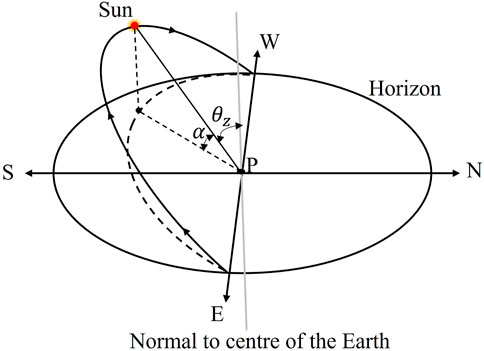
FIGURE 1. The altitude angle (α) and the zenith angle (${\theta }_Z$) of the sun when viewed from point P, and α+ ${\theta }_Z$ = 90°.

Therefore, we adopted the method recommended by the Food and Agriculture Organization of the United Nations (FAO) to estimate R_act, and then to improve the estimation method of the quantity of solar radiation at ground level.

According to the Angstrom formula (Allen et al., 1998), R_act is calculated as follows:

$R_{act}=\left(a_s+b_s\frac{n}{N}\right)\times R_a(6)$

where n represents the actual sunshine hours, N is the maximum possible sunshine hours, then n/N is the relative sunshine hours; and R_a is the solar radiation per unit area at the top of the atmosphere, namely the solar constant (MJ/m²/day); a_s is the regression constant, the fraction of solar radiation per unit area at the top of the atmosphere reaching the ground in cloudy weather conditions; a_s + b_s is the fraction of solar radiation per unit area at the top of the atmosphere in clear weather conditions. The values of the two parameters (De Freitas, 1979) are a_s = 0.25 and b_s = 0.5, respectively.

R_a is calculated by the following equation:

$R_a=\frac{24\times 60}{\pi }{G}_{sc}\times d_r\times \left[{\omega }_s\times \sin \phi \times \sin \delta +\cos \phi \times \cos \delta \times \cos {\omega }_s\right](7)$

R_a is the solar radiation per unit area at the top of the atmosphere (MJ/m²/day); G_sc is the solar constant (.082 MJ/m²/min); and d_r is the inverse of the relative distance between the Sun and the Earth; ${\omega }_s$ is the solar time angle in radians; $\phi$ is the local latitude in radians; δ is the solar magnetic declination in radians. The equation for d_r and $\phi$ are as follows:

$d_r=1+0.033\times \cos \left(\frac{2\pi }{365}J\right)(8)$

$\delta =0.409\times \sin \left(\frac{2\pi }{365}J-1.39\right)(9)$

where J is the number of day sequences for a day of the year, between 1 (1 January) and 365 or 366 (31 December).

${\omega }_s=\arccos \left(-\tan \phi \tan \delta \right)(10)$

$\left\{\begin{array}{c}J=fix\left(275\times \left(\frac{mth}{9}\right)-30+D\right)\\ Ifmth<3,J=J+2\\ Ifitistheleapyearandmth>3,J=J+1\end{array}\right.(11)$

where J is the number of day sequences for a day of the year, mth is the month, D is the specific date, and fix() is rounded.

The solar radiation per unit area at the top of the atmosphere R_a (MJ/m²/day) can be calculated based on Eq. 7, which needs to be converted to W/m² with a conversion factor of 11.6 provided by the FAO (Food and Agriculture Organization), therefore, based on Eq. 6, R_act (W/m²) can be obtained as follows:

$R_{act}=\left(a_s+b_s\frac{n}{N}\right)\times R_a\times 11.6(12)$

Therefore, ICL-new was obtained by combining Eqs 3, 4, 12. Theoretically, the ICL-new considers the impacts of seasonal and daily variations in solar activity on R_act and is more realistic than the original ICL. In this study, we used 31 provincial capitals in mainland China as research cases to compare the original ICL and ICL-new and determine the impact of applying the revised model.

The precision calculation of R_act

The simulated values of R_act include three types: R_act acquired using the FAO method, R_act obtained from the sine and cosine functions in the original ICL. The actual values of R_act are calculated using observed data from ground stations. Three evaluation indices, Nash–Sutcliffe efficiency coefficient (NSE), distance of indices between simulation and observation (DISO) (Zhou et al., 2021; Hu et al., 2022), and percentage deviation (P_bias), were selected to assess the precision of R_act estimated by the three methods. The three evaluation indices are expressed as follows:

$NSE=1-\frac{{\displaystyle \sum }_1^n{\left(Q_i^{obs}-Q_i^{sim}\right)}^2}{{\displaystyle \sum }_1^n{\left(Q_i^{obs}-\overline{Q_i^{obs}}\right)}^2}(13)$

$P_{bias}=\frac{{\sum }_1^n\left(Q_i^{obs}-Q_i^{sim}\right)}{{\sum }_1^n{Q}_i^{obs}}\times 100\%(14)$

$DISO=\sqrt{{NRMSE}^2+{RB}^2+{\left(R-1\right)}^2}(15)$

where $Q_i^{obs}$ and $Q_i^{sim}$ are the observed and simulated values of R_act at month i, respectively, $\overline{Q_i^{obs}}$ is the average value of the corresponding monthly R_act, and n is the length of time (months). NRMSE, RB and R are the normalized root mean square error, relative bias and Pearson correlation coefficient, respectively, which are described by the Hu et al. (2019).

The evaluation results can be categorized on a scale of very excellent, good, satisfactory, and unsatisfactory (Table 2). When the Nash–Sutcliffe efficiency (NSE) is closer to 1, and the absolute value of percentage deviation (P_bias) is more closer to 0, the simulation is better.

TABLE 2

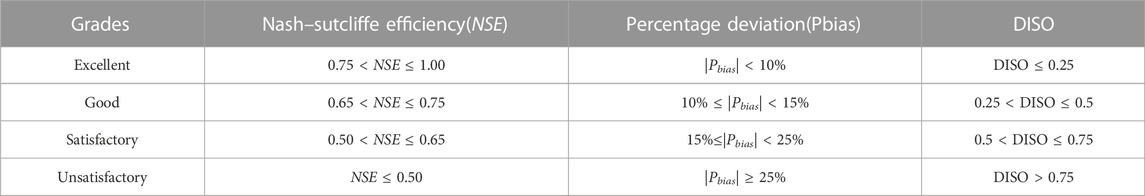
TABLE 2. Grading criteria based on the assessment of R_act in the ICL models.

Grading criteria for the ICL

Depending on the comfortable level of the clothing, the ICL is divided into five categories: extremely unsuitable, unsuitable, less suitable, more suitable, and most suitable. According to Ma et al. (2009), the grading symbolizes (i.e., A, B, b, C, c, D, d, E, e) the relative suitability of clothing and sensation of the human body corresponding to the various ICL values can be obtained (Table 3). When .5 < ICL ≤ 1.5, it means that the climate is neither too hot nor too cold, such that the human body feels comfortable, and the grading symbols are A, B, and b; when ICL ≤ .5, it indicates that the climate is hot, and the human body needs to clothes to cool off, and the grading symbols are C, D, and E; when ICL > 1.5, it means that the climate is cold, and the human body requires clothing to maintain a constant temperature, indicated by the grading symbols are c, d, and e.

TABLE 3

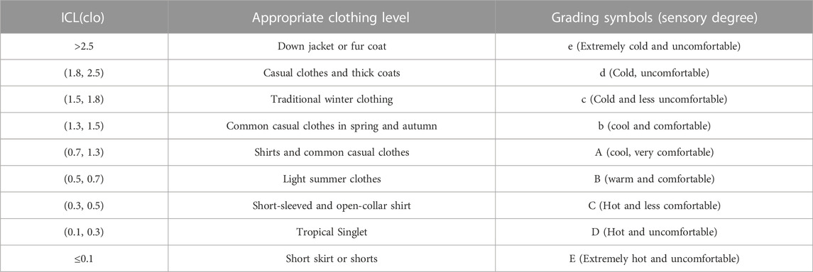
TABLE 3. Grading standards and appropriate clothing level for ICL (Ma et al., 2009).

Results and analysis

Evaluating the accuracy of R_act based on three methods

In the study, we used the monthly R_act obtained from nine ground-based solar radiation stations as observation data (noted as R_act-obs), which were used to assess the accuracy of R_act calculated using three different methods. R_act (noted as R_act-revised) was computed using the FAO algorithm, R_act (noted as R_act-sin) was calculated with the sine function based on Eq. 5, and R_act (noted as R_act-cos) was calculated using the cosine function. Results in Figure 2 indicated that the R_act-obs and R_act-revised values were extremely closely matched, with a similar distribution pattern within the year (Figure 2). R_act-cos calculations were modest in summer while prominent in winter, and they did not correspond to the annual cycle solar radiation change in the northern hemisphere. Although the R_act-sin calculations were compatible with the intra-annual fluctuation of solar radiation in the northern hemisphere, the values were excessive and significantly greater than the R_act-obs value. The R_act-cos and R_act-sin obtained from the ICL model greatly overestimated the solar radiation arriving at the Earth surface, mainly due to the method’s failure to account for latitudinal variation, seasonal and daily changes in surface solar radiation. Unlike the original ICL model, the R_act estimated by the FAO algorithm was more accurate.

FIGURE 2

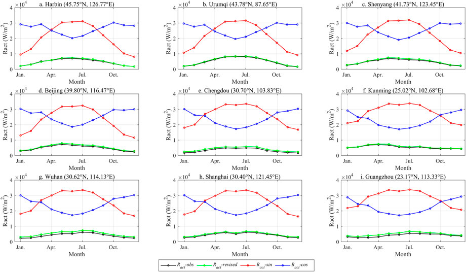
FIGURE 2. Comparative results of monthly R_act calculated by three methods. Lables (A–I) represent nine cities, Harbin, Urumqi, Shenyang, Beijing, Chengdu, Kunming, Wuhan, Shanghai, Guangzhou, respectively.

Meanwhile, we utilized the NSE and P_bais as assessment metrics, and the accuracy of R_act achieved by the three methods was quantitatively analyzed (Table 4). Based on the NSE assessment, the R_act-revised results indicated that excellent for six cities, good for one city, and two cities were unsatisfactory. Results based on the P_bais assessment showed that the precision of the R_act-revised was graded as excellent for four cities, good for two cities, satisfactory for three cities, and no cities were unsatisfactory results were produced. Results based on DISO assessment showed that the precision of the R_act-revised was graded as excellent for six cities, good for two cities, and no cities were unsatisfactory results were produced. Combining the findings of Figure 2 and Table 4, the R_act calculated by the R_act-sin and R_act-cos methods were dissimilar from the actual observed values, and their NSE, DISO and P_bais evaluations were also unsatisfactory. Consequently, the R_act-revised method produced results closer to the actual observed values than the R_act-sin and R_act-cos algorithms, which might be used to estimate R_act.

TABLE 4

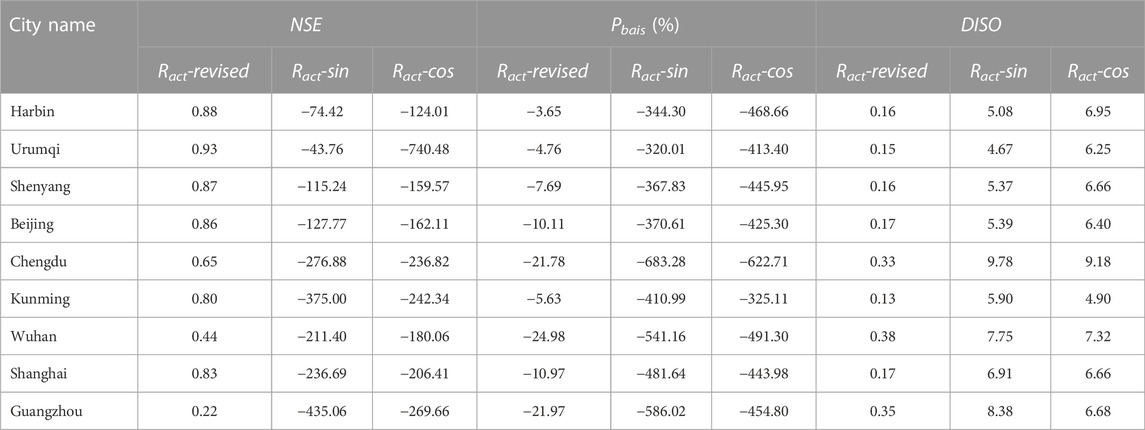
TABLE 4. The effectiveness assessment of the R_{act is} calculated by three methods.

Comparing the ICL calculated by three methods

To further confirm the reasonableness of the R_act-revised method, we calculated the multi-year monthly averages of three kinds of ICL for each of the nine cities using the R_act generated in the three ways described above. The ICL was produced using the R_act-revised, R_act-sin, and R_act-cos recorded as ICL-new, ICL-sin, and ICL-cos, respectively.

ICL-new (Figure 3) closely matches the intra-annual variation in temperature shown in Figure 4. As can be seen from the graphs of average monthly temperatures for each city over a multi-year period, the results of ICL-cos were inconsistent with reality, particularly in cities located at lower latitudes (Figure 3). The ICL-new and ICL-sin graphs (Figure 3) were similar, with good agreement in three cities Harbin (Figure 3A), Urumqi (Figure 3B), and Shenyang (Figure 3C), while values of ICL-sin were generally small in other cities. For example, the ICL-sin value for Beijing in January was approximately 1.5 (Figure 3), indicating that January is suitable for tourism. However, the average temperature in Beijing is below 0°C (Figure 4), which is not suitable for tourism. Furthermore, Chengdu’s ICL-sin in winter was below 0 (Figure 3), suggesting it is too hot although the monthly temperature (Figure 4) in winter is a reasonably comfortable 8°C–10°C, which is suitable for tourism. Therefore, this method was less appropriate for assessing climate change in the middle and low latitudes since the ICL-sin value was small. ICL-new produced more accurate results than ICL-sin and ICL-cos, which were generally consistent with intra-annual temperature changes.

FIGURE 3

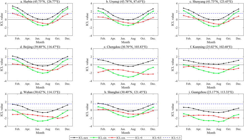
FIGURE 3. Comparison of multi-year monthly average ICL calculated by three methods in nine cities from 1981 to 2010. Lables (A–I) represent nine cities, Harbin, Urumqi, Shenyang, Beijing, Chengdou, Kunming, Wuhan, Shanghai, Guangzhou, respectively.

FIGURE 4

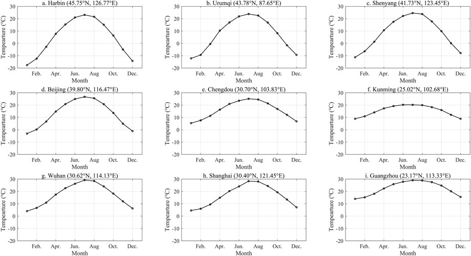
FIGURE 4. Multi-year monthly average temperature for nine cities during 1981–2010. Lables (A–I) represent nine cities, Harbin, Urumqi, Shenyang, Beijing, Chengdou, Kunming, Wuhan, Shanghai, Guangzhou, respectively.

A case study based on the improved ICL

To validate the ICL-new model, we evaluated the climate comfort of 31 provincial capitals in mainland China with ICL-new from 1980 to 2019 (Table 5). Results indicated the northern part of 33°N was comfortable in spring (March–May) and autumn (September–November) but uncomfortable in winter (December, January, February) and summer (June–August). The three capitals of Northeast China (Harbin and Changchun) were pleasant to visit during April–May and September–October. The climate comfort of those cities in the arid northwest (Urumqi, Xining, Lanzhou, and Yinchuan) varies widely, with Urumqi being ideal in April, September, and October, Xining in March-May and September-October, Lanzhou in February–March and November–December, and Yinchuan in March, April, and October. In the Loess Plateau region, Hohhot and Taiyuan were comfortable in April and October, whereas Xi’an was comfortable in March–April and October–November. The best times to visit cities North China (Beijing, Tianjin, Shijiazhuang, Jinan, and Zhengzhou) were March–April and September-October. Lhasa was suitable for tourists on the Qinghai-Tibet Plateau during May–September. Most southern cities were ideal in February–March and November–December (Table 5), while temperatures in the summer and autumn were unpleasant. High temperatures made the months of June, July, and August uncomfortable. Climate comfort cannot be fully interpreted by the ICL alone, as the ICL-new model indicated that the climate comfort in most southern Chinese cities was not high in April, while the weather in these cities was fine.

TABLE 5

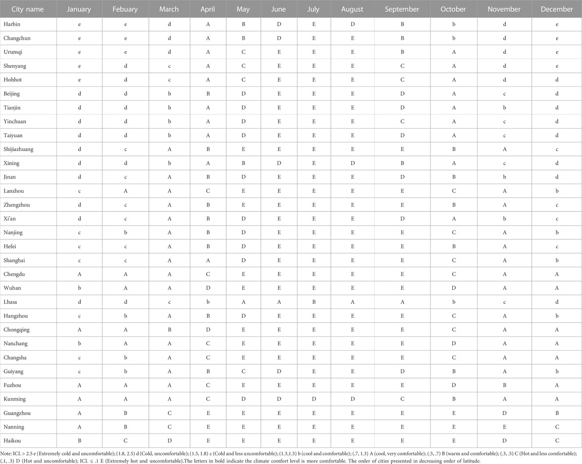
TABLE 5. Characteristics of the climate comfort in 31 mainland Chinese cities during 1980–2019 using ICL-new.

China’s annual average surface temperature has risen significantly since the mid-20th century, with a warming rate of .26°C/10a (Climate Change Center of China Meteorological Administration, 2021) which exceeds the global average over the same time frame. According to an analysis of the average ICL over the past 40 years, mainland China has experienced significant warming that has impacted the ICL and climate comfort. In terms of its physical meaning, an increase or decrease in the ICL reflects changes in climate comfort. Increasing or decreasing in the ICL corresponds to improves or deteriorates of climate comfort when the monthly ICL is less than .5. However, when the ICL is greater than 1.5, the increase or decrease in the ICL corresponds to deterioration or improvement of climate comfort. We used the Mann-Kendal non-parametric trend test method (Hamed, 2008) to calculate the trend in ICL for each month for all 31 cities from 1980 to 2019 (Figure 5). We found significant differences between the eastern and western cities in January, with a decreasing trend in ICL in the eastern cities and an increasing trend in the western cities (Figure 5), and a corresponding deterioration in climate comfort. The ICL of most cities in the middle and lower reaches of the Yangtze River (Changsha, Nanchang, Hefei, Nanjing, Zhejiang, Shanghai, etc.), North China (Zhengzhou, Jinan, Shijiazhuang, Beijing, and Tianjin) and Northeast China (Shenyang, Changchun, and Harbin) showed a decreasing trend in February (Figure 5), March (Figure 5) and April (Figure 5). According to Table 5, we could get higher values of the ICL in February, March, and April in these regions. Therefore, the descending trend suggests that climate comfort has improved over time. The ICL of most cities showed a decreasing trend for May–September (Figures 5E–I), and the climate comfort of most cities also deteriorated (Table 5). In October, ICL decreased in the middle and lower reaches of the Yangtze River indicating a deterioration in climate comfort (Figure 5J), while the decline in ICL in the northeast region indicated the climate comfort had improved over time. Changes in November and December were similar to those in January; the climate comfort in the eastern cities tended to improve, while the western cities tended to get worse.

FIGURE 5

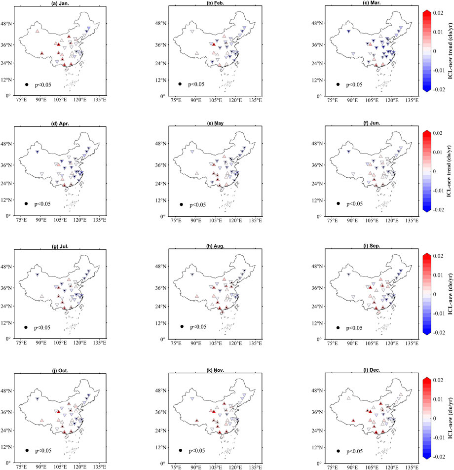
FIGURE 5. Spatial distribution of monthly changes of ICL-new during 1980–2019, the positive triangle indicates an upward trend, the inverted triangle indicates a decreasing trend, and the black dots indicate that the change in the ICL was significant at p = .05 level. Labels (A–L) represent January, February, March, April, May, June, July, August, September, October, November, December, respectively.

Discussion

The ICL calculation depends on the estimation of surface solar radiation. However, in the original ICL model, the estimation of surface solar radiation ignored seasonal variation and daily variation at the same location, resulting in an overestimation of surface solar radiation. We used the FAO surface solar radiation calculation method to improve the ICL model’s solar radiation estimation. Results showed that the FAO method’ simulated solar radiation were very close to the measurements, which can be used to improve the original ICL model. At the same time, the ICL-new has improved the shortcomings existed in evaluating climate comfort with the original dressing index model: Firstly, the overly macroscopic judgment of solar declination leads to overestimating estimated surface solar radiation in summer and underestimation in winter (Zhang et al., 2013; Cao et al., 2015; Sun and Yu, 2017); Secondly, a problem of wind speed unit conversion, which has been studied in cases where the wind speed (m/s) is directly substituted into the equation (Cao et al., 2015; Cao et al., 2019), ignoring that the wind speed unit in the original ICL model is cm/s, which should be converted from m/s to cm/s before substituted into the model. Therefore, we proposed a method to correct these two defects in the original ICL model, adopting the ICL-new model for an application.

Meanwhile, there are four urban observation stations in Shijiazhuang (Hebei), Lhasa (Tibet), Chengdu (Sichuan), and Chongqing (Chongqing) were not contained in the V3.0 dataset. For Shijiazhuang, we adopted Xingtai station; for Lhasa, we adopted Dangxiong station; for Chengdu, we adopted Wenjiang station; for Chongqing, we adopted Jiangjin station. Because the locations of the stations and cities do not match, there could be some uncertainty. For example, the index in Shijiazhuang uses other stations 100 km away, as there exists an urban island effect for big cities. There might be uncertainty in the results of R_act calculations at these stations, which in turn affects the accuracy of the ICL-new. This is one of the limitations of this study.

Temperatures have increased substantially in China since 1980s (Yu et al., 2015), and a warmer summer will result in a decreased in ICL (a worse climate comfort in summer) and the opposite is for a warmer winter. Meanwhile, the ICL model changed significantly under global warming, indicating that the static assessment of climate comfort used in the past (Hamed, 2008; Cao et al., 2019) is unsuitable. Thus, changes in the ICL model should be considered from the perspective of dynamic changes, which will help interpret climate comfort changes more comprehensively. We showed that global climate change significantly impacted climate comfort in 31 province capitals in mainland China. Of course, some limitations exist in evaluating climate comfort only by the ICL. For example, A (most comfortable) in April and E (extremely uncomfortable) in July for northeastern cities such as Harbin, Changchun, and Shenyang; A (most comfortable) in April and October and E (extremely uncomfortable) in July for northwestern cities, such as Xining and Urumqi; E in June, D (unsuitable) in September and A in October for Beijing; and A in March, April and November, D in May and C (less suitable) in October for Shanghai. For these cities, the ICL results did not match the temperature of the corresponding month. Therefore, for a comprehensive assessment of climate comfort, it is necessary to consider additional climate comfort indices (such as the Thermal Humidity Index and Wind Effect Index).

Conclusion

To improve the uncertainty of the original ICL, we recalculated solar radiation energy on the Earth’s surface by using the method recommended by the FAO, and validated the model based on meteorological data for 31 provincial capitals in mainland China. The main conclusions were as following.

1) The surface solar radiation derived from the improved method is significantly better than that in the original ICL model (NSE > .80, DISO < .25, and P_bais < 15%), and matches the seasonal variation of surface solar radiation. Surface solar radiation estimated by R_act-sin and R_act-cos method differed significantly from that observed; their NSE, DISO and P_bais were unsatisfactory. According to the R_act-revised calculations, values are very close to the actual observed values and can be used to estimate the amount of solar radiation reaching the ground.

2) The improved ICL model (ICL-new) is superior to the original ICL model (ICL-cos). The agreement between ICL-new and ICL-cos was only reasonable for three of Harbin, Urumqi, and Shenyang cities considered, while the values of ICL-cos in other cities are relatively small. The ICL-new model was more accurate than the original ICL-cos model particularly for mid to low latitudes in China.

3) In this study, the improved ICL-new was adopted to examine the climate comfort of 31 provincial capitals in mainland China from 1980 to 2019, results showed that climate comfort was lower in summer and became better in spring and autumn. Meanwhile, climate comfort improved over time for February–April, but it deteriorated between May and September. Climate comfort was worsened in China’s southern cities in October between 1980 and 2019, enhanced in northern cities, and further exacerbated in western cities in November, December and January.

Data availability statement

Publicly available datasets were analyzed in this study. This data can be found here: The daily-scale meteorological observation data were obtained from the “Daily Value Dataset of Climate Information from Ground-based International Exchange Stations in China (V3.0) (excluding data from Hong Kong, Macao and Taiwan)” provided by the National Meteorological Science Data Center (http://data.cma.cn/).

Author contributions

Conceptualization: QL, LL, and HD; methodology: HD, QL, and ZH; formal analysis: QL, HD, and YZ; data curation: QL, LL, and YZ; and writing—original draft preparation: QL, LL, and HD funding acquisition: QL and LL.

Funding

We declare all sources of funding received for the research being submitted, funds received for open access publication fees. Foundation items: This research was funded by Public Welfare Scientific Institutions of Fujian Province, No. 2021R1002001; National Natural Science Foundation of China, No. 41871146; Fujian Educational Research Project for Young and Middle-aged Teachers, No. JAT190085.

Conflict of interest

The authors declare that the research was conducted in the absence of any commercial or financial relationships that could be construed as a potential conflict of interest.

Publisher’s note

All claims expressed in this article are solely those of the authors and do not necessarily represent those of their affiliated organizations, or those of the publisher, the editors and the reviewers. Any product that may be evaluated in this article, or claim that may be made by its manufacturer, is not guaranteed or endorsed by the publisher.

Supplementary material

The Supplementary Material for this article can be found online at: https://www.frontiersin.org/articles/10.3389/fenvs.2022.992503/full#supplementary-material

Supplementary Figure S1 | 1980–2019 monthly temperature trend of 31 cities over mainland China.

References

Allen, R. G., Pereira, L. S., Raes, D., and Smith, M. (1998). Crop evapotranspiration guidelines for computing crop water requirements. FAO Irrigation and drainage paper 56. Rome: Food and Agriculture Organization. Available at: http://www.fao.org/docrep/x0490e/x0490e00.htm

Google Scholar

Atzori, R., Fyall, A., and Miller, G. (2018). Tourist responses to climate change: Potential impacts and adaptation in Florida's coastal destinations. Tour. Manag. 69, 12–22. doi:10.1016/j.tourman.2018.05.005

CrossRef Full Text | Google Scholar

Auliciems, A., and De Freitas, C. R. (1976). Cold stress in Canada: A human climatic classification. Int. J. Biometeorology 20, 287–294. doi:10.1007/BF01553585

PubMed Abstract | CrossRef Full Text | Google Scholar

Becken, S., Whittlesea, E., Loehr, J., and Scott, D. (2020). Tourism and climate change: Evaluating the extent of policy integration. J. Sustain. Tour. 28, 1603–1624. doi:10.1080/09669582.2020.1745217

CrossRef Full Text | Google Scholar

Blazejczyk, K., Epstein, Y., Jendritzky, G., Staiger, H., and Tinz, B. (2012). Comparison of UTCI to selected thermal indices. Int. J. Biometeorology 56, 515–535. doi:10.1007/s00484-011-0453-2

PubMed Abstract | CrossRef Full Text | Google Scholar

Burton, A. C., and Edholm, O. G. (1955). Man in a cold environment. London: Edward Arnold.

Google Scholar

Cao, K. J., Yang, Z, P., Meng, X. Y., and Han, F. (2015). An evaluation of tourism climate suitability in Altay Prefecture. J. Glaciol. Geocryol. 37 (5), 1420–1427. doi:10.7522/j.isnn.1000-0240.2015.0157

CrossRef Full Text | Google Scholar

Cao, Y., Sun, Y. L., and Wu, M. X. (2019). Spatial and temporal characteristics of the periods of climate comfort in the Beijing-Tianjin-Hebei region from 1966 to 2015. Acta Ecol. Sin. 39 (20), 7567–7582. doi:10.5846/stxb201805181096

CrossRef Full Text | Google Scholar

Climate Change Center of China Meteorological Administration (2021). Blue book on climate change in China 2021. Beijing, China: Science Press.

Google Scholar

Costa, M. L., Freire, M. R., and Kiperstok, A. (2019). Strategies for thermal comfort in University buildings—the case of the faculty of architecture at the federal University of bahia, Brazil. J. Environ. Manag. 239, 114–123. doi:10.1016/j.jenvman.2019.03.004

PubMed Abstract | CrossRef Full Text | Google Scholar

De Freitas, C. R., and Grigorieva, E. A. (2015). A comprehensive catalogue and classification of human thermal climate indices. Int. J. Biometeorology 59 (1), 109–120. doi:10.1007/s00484-014-0819-3

PubMed Abstract | CrossRef Full Text | Google Scholar

De Freitas, C. R. (1979). Human climates of northern China. Atmos. Environ. 13 (1), 71–77. doi:10.1016/0004-6981(79)90246-4

PubMed Abstract | CrossRef Full Text | Google Scholar

Deng, L. Z., and Bao, J. G. (2020). Spatial distribution of summer comfortable climate and winter comfortable climate in China and their differences. Geogr. Res. 39 (1), 41–52. doi:10.11821/dlyj020180792

CrossRef Full Text | Google Scholar

Dubois, G., Ceron, J. P., Gössling, S., and Hall, C. M. (2016). Weather preferences of French tourists: Lessons for climate change impact assessment. Clim. Change 136, 339–351. doi:10.1007/s10584-016-1620-6

CrossRef Full Text | Google Scholar

Feng, X., Sun, X., and Yu, Q. (2014). Anti-season tourism and tourism seasonality mitigation: Current research and relevant implications. Tour. Trib. 29, 92–100. doi:10.3969/j.issn.1002-5006.2014.01.010

CrossRef Full Text | Google Scholar

Fontan, S., and Rusticucci, M. (2021). Climate and health in buenos aires: A review on climate impact on human health studies between 1995 and 2015. Front. Environ. Sci. 8, 528408. doi:10.3389/fenvs.2020.528408

CrossRef Full Text | Google Scholar

Hamed, K. H. (2008). Trend detection in hydrologic data: The mann–kendall trend test under the scaling hypothesis. J. Hydrology 349 (3), 350–363. doi:10.1016/j.jhydrol.2007.11.009

CrossRef Full Text | Google Scholar

Höppe, P. (1984). Die Energiebilanz des Menschen. München: University of München.

Google Scholar

Hu, Z., Chen, D., Chen, X., Zhou, Q., Peng, Y., Li, J., et al. (2022). CCHZ-DISO: A timely new assessment system for data quality or model performance from da dao zhi jian. Geophys. Res. Lett. 49, 681. doi:10.1029/2022GL100681

CrossRef Full Text | Google Scholar

Hu, Z., Chen, X., Zhou, Q., Chen, D., and Li, J. (2019). Diso: A rethink of taylor diagram. Int. J. Climatol. 39 (5), 2825–2832. doi:10.1002/joc.5972

CrossRef Full Text | Google Scholar

Li, S., Sun, M. S., Zhang, W. J., Tan, L., Zhu, N. N., and Wang, Y. F. (2016). Spatial patterns and evolving characteristics of climate comfortable period in the mainland of China: 1961—2010. Geogr. Res. 35 (11), 2053–2070. doi:10.11821/dlyj201611005

CrossRef Full Text | Google Scholar

Liu, J., Huang, L., Sun, X. Q., Li, N. X., and Zhang, H. J. (2019). Impact of climate change on birdwatching tourism in China: Based on the perspective of bird phenology. Acta Geogr. Sin. 74 (5), 912–922. doi:10.11821/dlxb201905006

CrossRef Full Text | Google Scholar

Loehr, J., and Becken, S. (2021). The tourism climate change knowledge system. Ann. Tour. Res. 86, 103073. doi:10.1016/j.annals.2020.103073

CrossRef Full Text | Google Scholar

Lopes, H. S., Remoaldo, P. C., Ribeiro, V., and Martín-Vide, J. (2021). Perceptions of human thermal comfort in an urban tourism destination——a case study of porto (Portugal). Build. Environ. 205, 108246. doi:10.1016/j.buildenv.2021.108246

CrossRef Full Text | Google Scholar

Ma, L. J., and Sun, G. N. (2009). Evaluation on tourism climate comfort degree of hot cities in China. J. Shaanxi Normal Univ. Sci. Ed. 37 (2), 961672–1024291. doi:10.1155/2020/8886316

CrossRef Full Text | Google Scholar

Ma, L. J., Sun, G. N., and Wang, J. J. (2009). Evaluation of tourism climate comfortableness of coastal cities in the eastern China. Prog. Geogr. 28 (5), 713–722. doi:10.11820/dlkxjz.2009.05.009

CrossRef Full Text | Google Scholar

Ma, R. F., Zhang, W. Z., Yu, J. H., Wang, D., and Shen, L. (2014). Overview and prospect of research on human settlement of Chinese geographers. Sci. Geogr. Sin. 34 (12), 1470–1479. doi:10.13249/j.cnki.sgs.2014.12.008

CrossRef Full Text | Google Scholar

Pintassilgo, P., Rosselló, J., Santana-Gallego, M., and Valle, E. (2016). The economic dimension of climate change impacts on tourism. Tour. Econ. 22 (4), 685–698. doi:10.1177/1354816616654242

CrossRef Full Text | Google Scholar

Scott, D., Hall, C. M., and Gossling, S. (2019). Global tourism vulnerability to climate change. Ann. Tour. Res. 77, 49–61. doi:10.1016/j.annals.2019.05.007

CrossRef Full Text | Google Scholar

Sun, G. N., and Yu, Z, K. (2017). Relationship of climate comfort degree of cities near 30°N and 35°N with 3-step terrain of China. Arid. Land Geogr. 37 (3), 447–457. doi:10.13826/j.cnki.cn65-1103/x.2014.03.005

CrossRef Full Text | Google Scholar

Sun, M. S., and Li, S. (2015). Empirical indices evaluating climate comfortableness: Review and prospect. Tour. Trib. 30 (12), 19–34. doi:10.3969/j.issn.1002-5006.2015.12.007

CrossRef Full Text | Google Scholar

Terjung, W. H. (1966). Physiologic climates of the contentious United States: A bioclimatic classification based on man. Ann. Assoc. Am. Geogr. 5 (1), 141–179. doi:10.1111/j.1467-8306.1966.tb00549.x

CrossRef Full Text | Google Scholar

Willibald, F., Kotlarski, S., Ebner, P., Bavay, M., Marty, C., Trentini, F., et al. (2021). Vulnerability of ski tourism towards internal climate variability and climate change in the Swiss Alps. Sci. Total Environ. 784, 147054. doi:10.1016/j.scitotenv.2021.147054

PubMed Abstract | CrossRef Full Text | Google Scholar

Wu, J., Gao, X. J., Han, Z. Y., and Xu, Y. (2017). Analysis of the change of comfort index over Yunnan Province based on effective temperature. Adv. Earth Sci. 32 (2), 174–186. doi:10.11867/j.issn.1001-8166.2017.02.0174

CrossRef Full Text | Google Scholar

Yan, Y. C., Yue, S. P., Liu, X. H., Wang, D. D., and Chen, H. (2013). Advances in assessment of bioclimatic comfort conditions at home and abroad. Adv. Earth Sci. 28 (10), 1119–1125. doi:10.2478/s13533-012-0118-7

CrossRef Full Text | Google Scholar

Yu, D. D., Li, S., Zhang, L. F., Luo, Y., and Shi, Z. Y. (2021). Evaluate tourism climate using modified holiday climate index in China. Tour. Trib. 36 (5), 14–28. doi:10.19765/j.cnki.1002-5006.2021.05.007

CrossRef Full Text | Google Scholar

Yu, E. T., Sun, J. Q., Chen, H. Q., and Xiang, W. L. (2015). Evaluation of a high-resolution historical simulation over China: Climatology and extremes. Clim. Dyn. 45 (7-8), 2013–2031. doi:10.1007/s00382-014-2452-6

CrossRef Full Text | Google Scholar

Zhang, L. F. (2019). Tourism climate assessment: Model optimization and Chinese case. Shanghai: East China Normal University.

Google Scholar

Zhang, Y., Ma, M. J., Wang, S. G., and Shang, K, Z. (2013). Evaluation on tourism climate comfort in Nine famous mountain scenic spots in Chinese mainland. Meteorol. Mon. 39 (9), 1221–1336. doi:10.7519/j.isnn.1000-0526.2013.09.020

CrossRef Full Text | Google Scholar

Zhao, J., and Wang, S. (2021). Spatio-temporal evolution and prediction of tourism comprehensive climate comfort in Henan province, China. Atmosphere 12, 823. doi:10.3390/atmos12070823

CrossRef Full Text | Google Scholar

Zhong, L. S., and Chen, D. J. (2019). Progress and prospects of tourism climate research in China. Atmosphere 10 (11), 701. doi:10.3390/atmos10110701

CrossRef Full Text | Google Scholar

Zhou, Q., Chen, D., Hu, Z., and Chen, X. (2021). Decompositions of Taylor diagram and DISO performance criteria. Int. J. Climatol. 41 (12), 5726–5732. doi:10.1002/joc.7149

CrossRef Full Text | Google Scholar