Consistency of six in situ, in vitro and satellite-based methods to derive chlorophyll a in two optically different lakes

Phytoplankton and its most common pigment chlorophyll a (Chl-a) are important parameters in characterizing lake ecosystems. We compared six methods to measure the concentration of Chl a (C_Chl-a) in two optically different lakes: stratified clear-water Lake Saadjärv and non-stratified turbid Lake Võrtsjärv. C_Chl-a was estimated from: in vitro (spectrophotometric, high-performance liquid chromatography); fluorescence (in situ automated high-frequency measurement (AHFM) buoys) and spectral (in situ high-frequency hyperspectral above-water radiometer (WISPStation), satellites Sentinel-3 OLCI and Sentinel-2 MSI) measurements. The agreement between methods ranged from weak (R² = 0.26) to strong (R² = 0.93). The consistency was better in turbid lake compared to the clear-water lake where the vertical and short-term temporal variability of the C_Chl-a was larger. The agreement between the methods depends on multiple factors, e.g., the environmental and in-water conditions, placement of sensors, sensitivity of algorithms. Also in case of some methods, seasonal bias can be detected in both lakes due to signal strength and background turbidity. The inherent differences of the methods should be studied before the synergistic use of data which will clearly increase the spatial (via satellites), temporal (AHFM buoy, WISPStation and satellites) and vertical (profiling AHFM buoy) coverage of data necessary to advance the research on phytoplankton dynamics in lakes.

1 Introduction

Phytoplankton forms the basis of the aquatic food web (Fenchel, 1988), reacts fast to the changes in the environment (Reynolds, 2006; Hama et al., 2015), and reflects the alterations in climate (Winder and Sommer, 2012; Guinder and Molinero, 2013). The main photosynthetic pigment in phytoplankton is chlorophyll a (Chl a), which has hence been used for a long time as a metric for describing phytoplankton properties, either as a proxy for biomass (Vörös and Padisak, 1991; Boyer et al., 2009; Bernát et al., 2020), a measure of eutrophication (Ferreira et al., 2011; Matthews, 2014; Guan et al., 2020), an indicator for blooms (Reinart and Kutser, 2006; Gittings et al., 2017), or basis for primary production calculations (Longhurst et al., 1995; Tilstone et al., 2014). It is also one of the important parameters in assigning the ecological status class of water bodies by various legislative acts, e.g. Water Framework Directive (European Commission, 2000) and Marine Strategy Framework Directive (European Commission, 2008) both in pan-European scale and regional conventions, such as OSPAR (Convention for the Protection of the Marine Environment of the North-East Atlantic) or HELCOM (Baltic Marine Environment Protection Commission) (HELCOM, 2006; OSPAR Commission, 2009).

The variety of ways to determine the concentration of Chl a (C_Chl-a) is constantly increasing. In laboratory conditions, spectrophotometric method for C_Chl-a detection is widely used, although details in methodology (used solvent, calculation scheme, etc.) may differ among recommended standards and research groups (Gitelson et al., 2007; Zhang et al., 2009; Matthews et al., 2012; Pahlevan et al., 2020). High-performance liquid chromatography (HPLC) is by design more precise and has become a standard for analyzing phytoplankton pigments in marine and freshwaters (Simmons et al., 2016). Regardless of being relatively fast, objective and sensitive (Tamm, 2019), it is often unaffordable for smaller research teams or when high number of samples needs to be analyzed.

Automated high-frequency measurements (AHFM) of chlorophyll fluorescence with buoys equipped with various sensors, allow insight into processes within a lake in sub-hourly timescales (Laas et al., 2016). This enables the study of the diurnal and seasonal variations of C_Chl-a and lake metabolism in close details (Meinson et al., 2016) and provides a deeper insight into ecosystem dynamics, suits for assessing matter fluxes, and establishing precise chemical budgets (Rinke et al., 2013). AHFM systems are particularly useful to capture short-term events (e.g., cyanobacterial blooms) and fast water quality shifts in highly dynamic systems, together with enhancements in overall predictive capacity (Marcé et al., 2016). Profiling sensors in lakes give an overview of the vertical water column, while sensors deployed at fixed depths give information about one specific depth and location. Earlier, AHFM buoys were mainly equipped with underwater sensors to measure water temperature, electrical conductivity, pH, and dissolved oxygen properties, while information about biota, e.g., C_Chl-a, was much scarcer (Meinson et al., 2016; Meinson, 2017). Over the last decade, most of the new AHFM systems have at least some sensors to detect algal pigment changes, and therefore many studies have also explained C_Chl-a variability in lakes (Brentrup et al., 2016; Rusak et al., 2018). Continuous AHFM monitoring allows comprehensive studies of fast-evolving processes in lakes in short-term scales (Snortheim et al., 2017; Woolway et al., 2017). The presence of sensors in many lakes around the globe (e.g., via GLEON network) gives means to draw broader conclusions about the effects of changing climate and resulting factors. This is important from both scientific and management point of view.

Spectral radiometric measurements allow the quantification of C_Chl-a via the absorption and scattering features in the recorded signal. In situ hyperspectral optical sensors (e.g., WISPStation) provide high spectral and temporal resolution, which enables the validation of visible and near-infrared bands of present and future satellite missions providing water reflectance data within minutes (Vansteenwegen, et al., 2019). WISPStation is an optical measurement system deriving above-water reflectance (spectral range 350–900 nm, spectral resolution 4.6 nm) and in-water substances (Peters et al., 2018) e.g., C_Chl-a. High-frequency hyperspectral optical data can complement relatively scarce in situ measurements. This allows improving the knowledge about short-term processes in lakes and could be linked with Earth Observation (EO) measurements to increase knowledge in spatial scale (Siegel et al., 2013; Binding et al., 2018; Hu et al., 2019). EO data provides a frequent, large-scale synoptic overview of lakes and has been increasingly integrated operationally into inland water algal bloom monitoring (Binding et al., 2021). European Union’s EO Programme Copernicus currently provides data access up to four Sentinel series satellites to derive optical water quality parameters in lakes. Sentinel-3 (S3) Ocean and Land Colour Instrument (OLCI) offers an opportunity to monitor inland and coastal waters with high spectral (21 bands) and temporal (global coverage every 2 days) resolution. Still, it is more suitable for monitoring large water bodies because of its spatial resolution (pixel size 300 m on the ground). Another European Space Agency satellite Sentinel-2 (S2) Multispectral Instrument (MSI) allows monitoring smaller water bodies, with spatial resolution of 10–60 m on the ground, but has lower spectral, radiometric and temporal resolution compared to Sentinel-3 OLCI. Although Sentinel-2 was initially created for land applications, water quality parameters can be still successfully mapped (Toming et al., 2016; Pahlevan et al., 2017; Ansper & Alikas, 2018; Bonansea et al., 2019; Page et al., 2019; Al-Kharusi et al., 2020).

Various methods to derive C_Chl-a are widely used depending on the traditional monitoring methods, availability of the resources, instruments, specialists and laboratory facilities. Data gathered with different methods are then used to conclude the phytoplankton properties from regional to global scales (Sayers et al., 2015; Pahlevan et al., 2020), despite methodological differences within a dataset. The monitoring requirements of C_Chl-a by different methods can vary and depend on multiple factors. The expected accuracy is variable: for example for the fluorescence measurements by sonde, the manufacturer gives ±5% as the accuracy estimation. The photometric accuracy of spectrophotometer is dependent on absorbance range (±0.002 absorbance at 0 to 0.5 absorbance range; ±0.003 absorbance at 0.5 to one absorbance range). Sentinel-3 Copernicus requirements have set 10% accuracy goal for C_Chl-a for both Case 1 and Case 2 waters, while thresholds are 30% and 70% respectively, depending on the optical complexity of the waters (Drinkwater and Rebhan, 2007). Here we have used a comprehensive dataset where C_Chl-a has been measured simultaneously by several methods, commonly used in limnology and satellite-based estimations. Despite high temporal frequency of some methods (e.g., AHFM of fluorescence for 24 h, radiometric measurements up to 10 h (depending on Sun elevation)), the focus is set on midday measurements to allow the minimum time gap between all methods constrained by satellite overpasses and in vitro sample analyses in the laboratory. In this study, we compared six different methods to derive CChl-a values, and analyzed the linkage and merging between different methods to estimate the consistency of the methods to derive CChl-a in two optically different lakes.

2 Materials and methods

2.1 Study lakes

Lake Võrtsjärv is a shallow eutrophic lake located in the southern part of Estonia (Table 1; Figure 1). The water in the lake is generally well mixed, and there is no significant stratification. The dominant algal groups are diatoms and cyanobacteria (Limnothrix planctonica and L. redekei tend to dominate during the entire year), the rest (green algae, cryptophytes and dinoflagellates) belong to a minority group (Järvet and Nõges, 1998).

TABLE 1

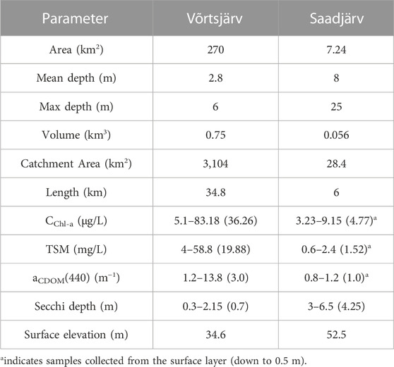
TABLE 1. Main morphological and bio-optical parameters in Võrtsjärv and Saadjärv. Mean values are given in parentheses. TSM refers to total suspended matter (mg/L) and a_CDOM(442) to the absorption of coloured dissolved organic matter at 440 nm.

FIGURE 1

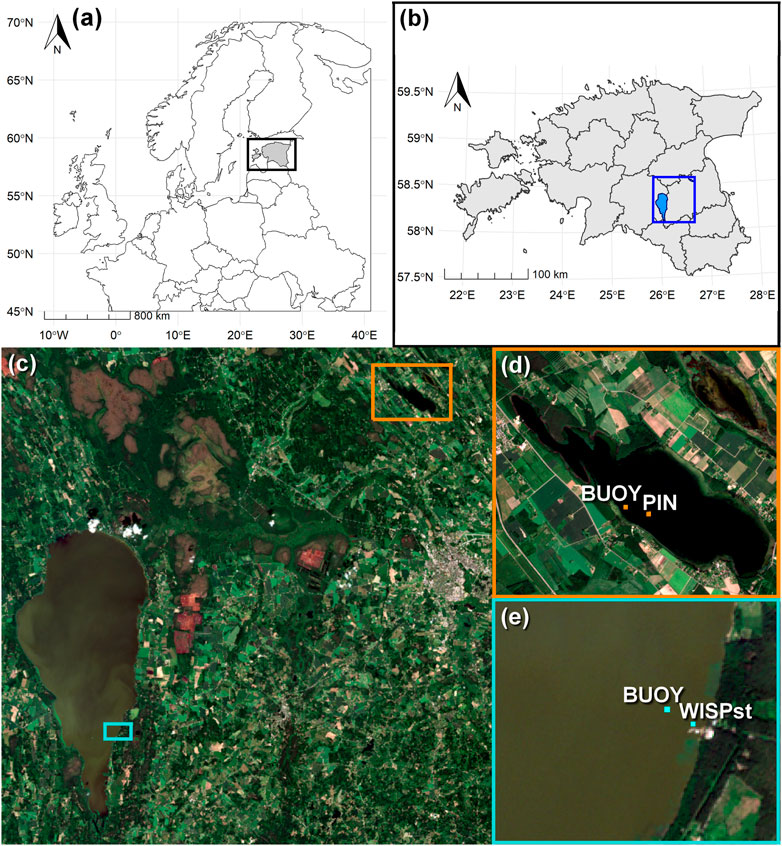
FIGURE 1. Location of the studied lakes on European scale (A) and within Estonia (B). The location of AHFM buoy and pin location for the satellite data in Saadjärv are in the image with orange frame (C,D). The location of WISPStation and AHFM buoy in Võrtsjärv are in light blue frame (C,E). Estonian contour was obtained from the Estonian Land Board (2021).

Lake Saadjärv is a relatively deep (maximum 25 m) mesotrophic lake in South Estonia. It is dimictic, and is stratified for most of the year (Cremona et al., 2016), with significant temperature differences between the surface and bottom layer, especially in summer. The dominant algal groups by biomass are diatoms, cryptophytes, and cyanobacteria.

Both lakes differ greatly in terms of the amount of optically active substances (Table 1), the resulting underwater light field and seasonal dynamics in phytoplankton. Võrtsjärv has typically increasing phytoplankton biomass towards autumn, while in Saadjärv phytoplankton is more abundant in spring. Võrtsjärv has almost an order of magnitude higher C_Chl-a mean value compared to Saadjärv (36.3 μg/L and 4.8 μg/L respectively, Table 1). Absorption of colored dissolved organic matter (a_CDOM) is higher in spring in both lakes and decreases towards autumn. Total suspended matter (TSM) increases towards autumn in Võrtsjärv (from ∼10 mg/L to 30 mg/L in 2018 and up to 40 mg/L in 2019) compared to low concentrations (∼1.5 mg/L) during the entire year in Saadjärv.

2.2 Data

2.2.1 Laboratory measurements

Water samples for C_Chl-a analyses were gathered from surface water (e.g., 0.5 m depth) in Saadjärv and from various depth integrated water (surface, then after every 0.5 m) in Võrtsjärv. Water samples were kept in the dark and cooled container and filtered during the same day of the fieldwork.

Duplicate samples for C_Chl-a were filtered onto 25 mm ø GF/F filters (0.7 μm pore size). Filters were stored at −20°C until being extracted with 5 ml 96% ethanol for 24 h, centrifuged for 10 min (4,000 rpm), measured spectrophotometrically (Hitachi, 2020) and C_Chl-a was calculated for mixed phytoplankton assemblage according to Jeffrey and Humphrey (1975).

For HPLC analysis, 100–700 ml of sampled lake water was vacuum filtered through 47-mm Whatman GF/F, triplicate filters were stored in 5 ml plastic vials, frozen immediately and kept at −70°C before analysis. Phytoplankton pigments were extracted in 100% acetone (2 ml) containing internal standard and sonicated (Branson 1210) for 5 min. Samples were stored at −20°C for 24 h. After that, the extracts were filtered through 0.45 μm syringe filters (Millex LCR, Millipore) and stored in dark refrigerator until HPLC analysis (for details, see Tamm et al., 2015). C_Chl-a and Chlorophyllide a values were summed up for total C_Chl-a.

2.2.2 Fluorescence measurements

Data from two AHFM buoy stations measuring fluorescence were used (Figure 1). Võrtsjärv AHFM buoy (58.211798 N, 26.103163 E) was equipped with a Yellow Springs Instruments (YSI) model 6600 V2-4 multiparameter sonde in 1-m depth. The sonde has been fitted with a chlorophyll fluorescence probe (model 6025) and was recording after every 10 min frequency. Saadjärv AHFM buoy station (58.536963 N, 26.647558 E) was equipped with a YSI EXO-2 multiparameter sonde and worked as a vertical profiler within 2–20 m water column. This sonde was fitted with an EXO Total Algae-Phycocyanin sensor. The buoy was set to make profiles after every 30 min in 2018 and 1-h frequency in 2019, from surface to bottom and the data was recorded every 4–5 cm. The automated sensor-based measurements of chlorophyll fluorescence (ChlF) was converted into C_Chl-a using standard manufactory coefficient and local conversion factors, derived via linear interpolation from monthly in vitro spectrophotometrically measured C_Chl-a. All underwater sensors in both AHFM systems were calibrated at least once per month according to the manufacturer instructions.

Both AHFM systems were also equipped with the multiparameter weather stations (Vaisala Weather Transmitter WXT520 in Võrtsjärv; Airmar 200WX Weather Station Instrument in Saadjärv) and solar irradiance sensors for above-water measurements. Photosynthetically active radiation (PAR) for Saadjärv was recorded with a Li-Cor quantum sensor (model LI-190SZ), while in Võrtsjärv, the buoy was equipped with a Li-Cor pyranometer (model LI-200SA), where PAR was calculated as 0.436 x Q (Q—incident global radiation) (Reinart and Pedusaar, 2008).

The non-photochemical quenching (NPQ) correction was performed according to Moiseeva et al. (2020):

${PAR}_z={PAR}_0\times e^{-\left(K_d\times z\right)}(1)$

$d_{op}=e^{\left(-0.0019\times {PAR}_z\right)}(2)$

$F_{real}=F_t\times \left({2-d}_{op}\right)(3)$

where PAR_z is photosynthetically active radiation, which penetrates to depth z, PAR₀ is PAR falling to the lake surface, K_d is a diffuse attenuation coefficient, d_op is a portion of the open reaction centres (photosystem 2), F_t is a quasi-stationary level of fluorescence in an object adapted to light and F_real is a corrected chlorophyll fluorescence. In Võrtsjärv, K_d was obtained from the WISPStation radiometric data (Alikas et al., 2015). In Saadjärv, in situ measured Secchi depth was used to derive the euphotic depth (Z_eu) as a ratio between coefficient 2.69 and Secchi depth (Luhtala and Tolvanen, 2013), which was then converted to K_d (Koenings and Edmundson, 1991). The corresponding Z₉₀ depth (depth at which 90% of the surface downwelling irradiance is attenuated) and Z_eu (reflects the depth where PAR is 1% of its surface value) were derived.

2.2.3 Spectral measurements

Fixed WISPStation was located in the pier of Võrtsjärv (Figure 1E, 58.211186 N, 26.107979 E). The station contains three radiometers that measure radiance and irradiance under fixed angles (Peters et al., 2018) with 15-min frequency. For a detailed description of the measurement setup, data processing and calibration of WISPStation, see Peters et al. (2018). Processed WISPStation data was downloaded from the WISPweb (https://wispweb.waterinsight.nl), where C_Chl-a has been calculated from derived reflectance according to Gons (1999). Data was filtered based on the solar zenith angle (>70°), and exceptionally high values of C_Chl-a (>200 μg/L), not consistent with the known natural background, were removed.

Satellite images from S2 MSI and S3 OLCI were used. Data was downloaded from Estonian National Satellite Data Centre ESTHub (ESTHub, 2022) with a pixel size of 60 m for S2 MSI and 300 m for S3 OLCI. First, S2 and S3 L1 data were processed with IDEPIX in SeNtinel Application Platform (SNAP) and pixels marked with cloud, cloud ambiguous, cloud sure, cloud buffer, cloud shadow, snow_ice and Sun glint risk flags were removed. Next, lake specific C_Chl-a algorithms were applied (Table 2).

TABLE 2

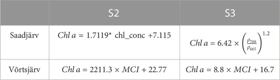
TABLE 2. Selected algorithms for Sentinel-2 MSI and Sentinel-3 OLCI data over study lakes.

Previous studies (Mograne et al., 2019; Pereira-Sandoval et al., 2019; Warren et al., 2019; Alikas et al., 2020) have shown that C2RCC and POLYMER (Steinmetz et al., 2011) tend to work relatively well compared to other available atmospheric correction methods on MSI and OLCI data over optically different waters. The atmospherically corrected data, standard C_Chl-a products from these processors together with previously developed approaches, based on L1 data (Alikas et al., 2015; Ansper and Alikas, 2018; Alikas et al., 2020), were tested over both lakes in terms of their accuracy and data availability.

In eutrophic Võrtsjärv (mean C_Chl-a 36.3 μg/L, TSM 19.9 mg/L, a_CDOM(440) 3.0 m⁻¹), L1 data based C_Chl-a retrieval showed to be more robust and resulted in more retrievals than atmospherically corrected L2 or any standard product for deriving C_Chl-a. Therefore, the Maximum Chlorophyll Index (MCI) (Gower et al., 2008) was applied to L1 data and C_Chl-a was derived by using empirical algorithms from S2 and S3 data in Võrtsjärv (Table 2).

In mesotrophic Saadjärv (mean C_Chl-a 4.8 μg/L, TSM 1.5 mg/L, a_CDOM(440) 1.0 m⁻¹), for S2 data POLYMER products resulted only in two quality controlled points in 2018 and four points in 2019, therefore C2RCC was chosen. C2RCC processor’s standard C_Chl-a product (chl_conc) with regional conversion factors was applied to S2 data. Also various empirical approaches were tested but due to high uncertainties in the shape and in the magnitude of the water-leaving reflectance from C2RCC, it did not result in more accurate C_Chl-a retrievals. For S3 data, POLYMER atmospheric correction was applied to derive remote sensing reflectance (ρ) and a ratio of 709 and 665 after Gilerson et al. (2010) was applied with lake-specific coefficients (Table 2).

For S2 and S3 images, 3 × 3 pixel area centered at the coordinates (ROI—region of interest) of the in situ stations were extracted for further analyses (Figure 1). The mean (µ) and standard deviation (σ) were calculated within the ROI. Each ROI was checked for outliers following the OLCI validation guidelines (EUMETSAT, 2019). Single pixel outliers were removed if C_Chl-a < (µ—1.5σ) or C_Chl-a > (µ + 1.5σ). Entire ROI was excluded when the ratio between standard deviation and mean e.g., coefficient of variation (CV), was greater than 0.2 (e.g. 20%).

2.3 Temporal frequency of data

Depending on the setup of the different AHFM systems (WISPStation, fixed/profiler buoy) they provided from 50 to 900 measurements daily, covering more than 100 days of data during the vegetation period (Table 3). Availability of satellite data was mainly regulated by cloud cover and combination of signal strength versus lake size, which resulted on average in 40 images over Võrtsjärv compared to 15 over Saadjärv (Table 3).

TABLE 3

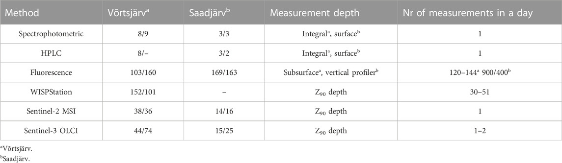
TABLE 3. Number of days with data used in this study. Slash (/) separates observations from years 2018 and 2019.

2.4 Statistical analyses

Open-source software tool R was used for statistical analyses and graphics. Bias and error between different methods were estimated according to Seegers et al. (2018):

$bias={{10}^{\wedge }}^{\left(\frac{{\displaystyle \sum }_{i=1}^n{\mathit{log}}_{10}\left(M_i\right)-{\mathit{log}}_{10}\left({Ref}_i\right)}{n}\right)}(4)$

$MAE={{10}^{\wedge }}^{\left(\frac{{\displaystyle \sum }_{i=1}^n\left.{\left|\mathit{log}\right.}_{10}\left(M_i\right)-{\mathit{log}}_{10}\left({Ref}_i\right)\right|}{n}\right)}(5)$

where M_i is a model value, Ref_i is a reference value, and n is a number of paired observations. Bias represents log-transformed residuals, whereas MAE stands for the mean absolute error computed in log-space. These metrics are dimensionless, where the value of 1.5 indicates the model predicted value is 50% higher on average than the reference in case of bias and relative measurement error is 50% in case of MAE.

Mean Absolute Percentage Difference (MAPD) was used to study the short-term variability in respect of the midday reading

$MAPD=\frac{{\displaystyle \sum }_{i=1}^{n}100\left|\frac{x_{midday,i}-x_{day,i}}{x_{midday,i}}\right|}{n}(6)$

where x_midday,i is a C_Chl-a reference value on a midday (12.30 GMT+3), x_day,i C_Chl-a value before or after midday, n is a number of observations.

The non-parametric two-sample Mann-Whitney U test was used to detect statistically significant differences between paired measurements.

3 Results

We first show the results from the inter-comparison of all methods in both lakes and in a second step analyze the consistency between the methods in lakes separately in terms of the changing environmental and in-water background conditions. Third, based on the spectral and fluorescence high frequency measurements, the causes for seasonal bias and outliers between two methods are demonstrated.

3.1 Method based comparison to derive C_Chl-a in two optically different lakes

The combination of seasonal dynamics (Figure 2) and pairwise comparison (Figure 3) showed smaller differences between the methods in eutrophic Võrtsjärv compared to Saadjärv (Table 4). The bias between different methods was smaller in Võrtsjärv (average 3%, up to 31%) compared to Saadjärv (average 27%, up to 55%). Similarly, the average MAE was smaller in Võrtsjärv (average 28%, with a range from 7% to 51%) compared to Saadjärv (average 97%, with a range from 51%–159%) (Table 4). While the sparse in vitro measurements showed generally good agreement with all available methods, the results were more scattered between spectral and fluorescence measurements.

FIGURE 2

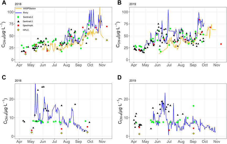
FIGURE 2. Midday C_Chl-a time-series during vegetation period of 2018 and 2019, derived from various sensors in Võrtsjärv (A,B): AHFM buoy, WISPStation, HPLC, spectrophotometric, S3, S2; and in Saadjärv (C,D): AHFM buoy at Z₉₀ depth, HPLC, spectrophotometric, S3, S2. Note the different y-scale in figures.

FIGURE 3

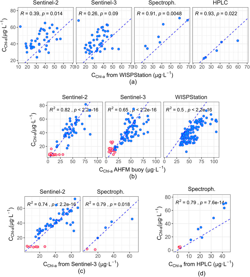
FIGURE 3. Comparison of C_Chl-a (µg·L⁻¹) acquired by various methods in Võrtsjärv (blue dots) and Saadjärv (red dots): (A) C_Chl-a from WISPStation in comparison with S2 (1), S3 (2), spectrophotometry (3) and HPLC (4), (B) C_Chl-a from fluorescence in comparison with S3 (1), S2 (2) and WISPStation (3), (C) C_Chl-a from S3 in comparison with S2 (1) and spectrophotometry (2) and (D) C_Chl-a from HPLC in comparison with spectrophotometry. R2 denotes the coefficient of determination about the entire dataset.

TABLE 4

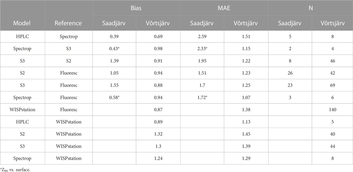
TABLE 4. Evaluated bias and mean absolute error (MAE) between studied methods according to Eqs 4, 5.

3.1.1 Laboratory measurements

Comparison of in vitro methods showed generally higher C_Chl-a by spectrophotometric approach compared to HPLC (Figure 3D). HPLC readings were, on average, 31% lower than spectrophotometrically measured C_Chl-a in Võrtsjärv (Table 4). In Saadjärv, the discrepancy was even more considerable.

The difference between the in vitro methods reflected also in the comparison with other methods. Comparison with WISPstation data showed underestimation of spectrophotometric C_Chl-a (24% bias, 29% MAE) and overestimation of HPLC C_Chl-a (11% bias, 13% MAE).

Compared to all methods, the smallest bias and MAE were derived between spectrophotometric and S3 (e.g., 2% bias in Võrtsjärv) and fluorescence (e.g., 6% bias in Võrtsjärv) based estimates in both lakes (Table 4).

3.1.2 Fluorescence measurements

In both lakes, the AHFM on ChlF delivered more than 100 days of data per year to study the seasonal dynamics of phytoplankton. As seen on Figure 2, the changes can be with high magnitude and rapid (e.g., daily changes in C_Chl-a ∼10 μg/L in Saadjärv and ∼30 μg/L in Võrtsjärv). This seasonal dynamics is well captured by all methods with varying measurement frequency in Võrtsjärv (Figure 2A, B) with a bias from 6%–13% and MAE from 7%–38% in respective to fluorescence measurements (Table 4). In Saadjärv, there is a clear difference between the S2 and S3 derived seasonal dynamics (Figures 2C, D), with S3 tends to follow more similar pattern with fluorescence measurements than S2. It resulted in statistically significant different retrievals with 55% bias and 70% MAE.

In terms of the fluorescence measurements, in both lakes, the difference between the midday and night-time ChlF increased with increasing phytoplankton amount. Night-time ChlF tends to be higher during more abundant phytoplankton e.g. during the spring bloom in Saadjärv (up to 5.9 RFU) and late summer bloom in Võrtsjärv (up to 1.7 RFU). With this in mind, statistics between all methods in respective to ChlF night measurements were derived, which showed that the daytime ChlF measurements resulted in better consistency in eutrophic Võrtsjärv with all methods. In Saadjärv, the differences in the derived statistics were small and more data would be needed to study the impact of choosing between night or daytime ChlF as a reference data.

The comparison of in-water fluorescence measurements showed that the short-term temporal variability was 60% higher on average in the clear water Saadjärv (MAPD 11%) than in turbid Võrtsjärv (MAPD 4.5%) within the ±30 min time interval (Supplementary Figure S1). While in Saadjärv the short-term variability in recorded ChlF measurements was higher during spring bloom (in both day and night measurements), no seasonal dependence respective to the phytoplankton quantity was observed in Võrtsjärv. In comparison, spectral data (i.e., WISPStation) showed higher standard deviation around the midday measurements towards autumn—during low light conditions. The comparison of in-water fluorescence and above-water radiometric methods in Võrtsjärv showed the in-water measurements tend to be more stable while the above-water measurements are more prone to outliers (Supplementary Figure S1).

3.1.3 Spectral measurements

Despite the methodological similarities in deriving C_Chl-a from WISPStation, S2 and S3 data, the comparison showed statistically significant differences, high scatter (Figures 3A1,2) and error up to 45% (Table 4) between WISPStation and EO data. Consistency was better between EO approaches in Võrtsjärv (Figure 3C; Table 4). In Saadjärv, although S2 and fluorescence measurements resulted in smallest bias (5%) and error (51%) from all methods in Saadjärv (Table 4), the C2RCC derived C_Chl-a estimates from S2 data resulted in fairly stable phytoplankton seasonal dynamics (Figures 2C, D) which was not supported by S3 and fluorescence based data.

In terms of spatial variability within the ROI, it was higher in Saadjärv during periods with more abundant phytoplankton (i.e. spring), but there were no systematic seasonal differences in S2 and S3 data over Võrtsjärv despite of the distinctive periods with higher C_Chl-a (Figures 2A, B).

The data from two AHFM systems (WISPstation and fluorescence buoy) in Võrtsjärv, resulted in 140 simultaneous measurements over 2 year period. Despite their moderate agreement (R² = 0.5), C_Chl-a from WISPStation was statistically significantly lower (on average 26%) than from fluorescence measurements (Table 4), larger values (>80 μg/L) were especially underestimated (Figure 3). Based on the statistics (Table 4), the fluorescence derived C_Chl-a tends to have better consistency with other methods than radiometric WISPStation measurements.

3.2 Environmental and in-water background conditions

In vitro measurements have been mainly performed in good measurement conditions (low wind speed, low wave height) which can partly explain their good agreement with other available methods.

Pairwise comparison of C_Chl-a estimates from radiometric (WISPStation, S2, S3) and fluorescence (buoy) measurements were coupled with buoy time series of observations of in-water and environmental conditions to determine their impact on the consistency of C_Chl-a retrievals. Here again, the impact of the environmental and background conditions during the measurements had different effect in eutrophic shallow Võrtsjärv and in stratified mesotrophic lake Saadjärv.

The increase in turbidity (due to C_Chl-a and TSM) tends to increase the differences between the methods in Võrtsjärv (Figure 4). This is evident especially in case of WISPStation data, whose C_Chl-a tend to be smaller compared to S2, S3 and fluorescence retrievals during elevated turbidity. This results in an increasing systematic bias between fluorescence and WISPStation data. Similarly, the increase in wind speed, causing surface distortions (foam, waves, glint) and resuspension from the bottom, has an impact on WISPStation data but it also explains the switch from under- to overestimation of values in case of fluorescence and S3 data. Due to the location of the WISPStation (Figure 1E), poorer consistency with other methods is observed in case of northerly winds, when subsurface scum and foam are transported along the pier. High flux densities in July and August, and low flux densities in September and October explain some of the outliers. In Võrtsjärv, the consistency between S2 and S3 tend to have lowest impact from the environmental and background conditions.

FIGURE 4

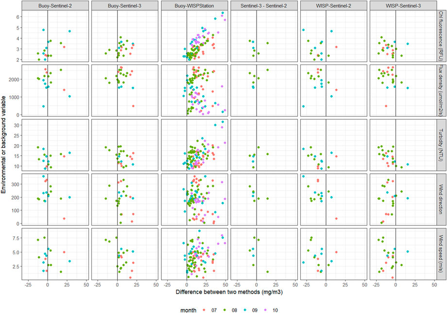
FIGURE 4. Impact of environmental and background conditions to method-based differences in estimating C_Chl-a in Lake Võrtsjärv.

In stratified clear water Saadjärv, the consistency between S2, S3, fluorescence measurements tend to depend largely on the signal strength e.g. ChlF and wind speed (Figure 5). The agreement between S2 and S3 decreases with decreasing ChlF, indicating the need for better algorithms for lower level of C_Chl-a. The dependence on signal strength is reflected also in the comparison of EO data with fluorescence measurements indicating larger biases during lower C_Chl-a. The low background turbidity (lower a_CDOM and TSM compared to Võrtsjärv, Table 1) results in higher amount of light available for phytoplankton in the subsurface layer and leads up to 81% change in ChlF due to the NPQ correction in Saadjärv. This could explain higher differences between fluorescence and spectral data during high flux density conditions, when the correction has the highest impact (Supplementary Figure S2). Despite the need for improved algorithms, the results also indicate improved consistency between fluorescence and EO based retrievals in case of increased wind speed, e.g. due to increased vertical mixing.

FIGURE 5

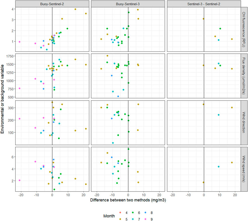
FIGURE 5. Impact of environmental and background conditions to method based differences in estimating C_Chl-a in Lake Saadjärv.

3.3 Method based differences to explain the seasonal bias and outliers

The inherent differences in the methods affect the consistency of C_Chl-a retrievals and might therefore result in seasonal bias. For example, monthly-based difference in the consistency between fluorescence and WISPStation C_Chl-a retrievals (Figure 6) could be explained by combined effect of various factors. First, timing of the in situ measurements to calibrate ChlF readings in high seasonal dynamics condition (Figure 2A). Second, increase of turbidity impacts both ChlF readings and sensitivity of the C_Chl-a algorithm applied on WISPStation radiometric data. Third, outliers in September and October can be explained with low light and high wind speed conditions, while outliers in July and August more by wind direction (Figure 4). Fourth, higher short-term variability in WISPStation data in autumn measurements with more noise in the radiometric data during low light conditions increases the uncertainty of the measurements.

FIGURE 6

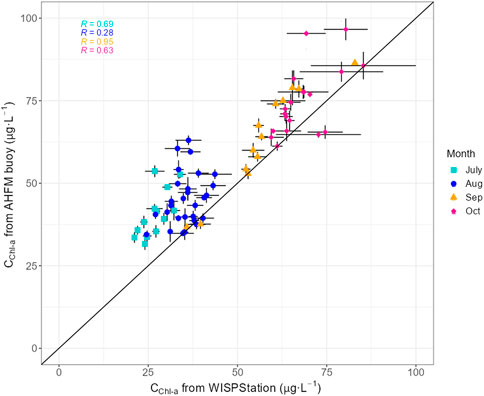
FIGURE 6. Hourly averaged and respective standard deviation for C_Chl-a derived from fluorescence (y-axis) and C_Chl-a derived from the spectral WISPStation data (x-axis) in Võrtsjärv during July-October 2018. Different months are coded with different colours. Time GMT+3 is used.

4 Discussion

The advancement of phytoplankton monitoring possibilities by various sensors requires the inter-comparison exercises to analyse the consistency of methods and outline the biases. The evaluation of C_Chl-a derived by six methods over 2-year time period in optically different lakes indicated the importance to consider both environmental and method-based factors while interpreting the results.

4.1 Method-based factors affecting C_Chl-a retrievals

4.1.1 Fluorescence measurements

There are various methods available to estimate the C_Chl-a from the ChlF measurements (Ferreira et al., 2012; Zeng et al., 2017). The fluorescence yield per chlorophyll unit is very variable and depends on phytoplankton community composition, cell size, packaging effect and NPQ (Carberry et al., 2019 and references therein) and is difficult to account for regular basis. This is especially a challenge in the waters where phytoplankton community consists of many different species and various life cycle phases are present.

High-frequency measurements allow obtaining information from ChlF in sufficient temporal scale relevant to natural dynamics of the phytoplankton community. Photoprotection against high light induced by the xanthophyll cycle will lead to a non-photochemical quenching. The effect of NPQ correction clearly increased with increased PAR (Kromkamp et al., 2008; Ruban, 2016) and also depended on the level of OAS (optically active substances), leading up to 15% change in ChlF readings in Võrtsjärv compared to 81% in Saadjärv (Supplementary Figure S2). The amount of PAR of the total solar radiation depends on the wavelength, solar zenith angle, the aerosol amount in the atmosphere and clouds (Ross & Sulev, 2000). In Estonian geographic location the monthly total PAR is highest in June and decreases towards spring and autumn (Russak & Kallis, 2003). Here we showed the consistency between C_Chl-a derived from above water radiometry (S2, S3, WISPStation) and fluorometers tended to decrease during high flux intensities in summer, especially pronounced in clear water Saadjärv (Figure 5). On the contrary, during autumn, when the illumination conditions were poorer, the consistency between the same methods was better during high flux intensities and decreased during low flux intensities (Figure 4). While in Võrtsjärv day-time ChlF was better reference based on the derived statistics (results not shown here), there was no clear pattern in Saadjärv. As the night-time ChlF tends to be higher during the bloom period and the difference was substantially higher in Saadjärv (up to 230%) compared to Võrtsjärv (up to 40%), it should be studied further in conjunction with inter-comparison of different methods to account for the NPQ.

It has been shown that CDOM and non-algal particles impede the accurate estimation of Sun-induced ChlF from the total reflectance spectra (McKee et al., 2007; Gilerson et al., 2008). Despite, the results from eutrophic Võrtsjärv show a strong correlation between C_Chl-a derived from below water fluorometry and above-water radiometry (Figure 6), it was also shown that both methods depend on the background turbidity (Figure 4). Proctor & Roesler (2010) and Kuha et al. (2020) outlined that organic matter may lead to an underestimation of C_Chl-a by absorbing excitation or emission wavelengths or, on the other hand, cause seemingly intensified Chl emission by contributing to the signal detected by Chl fluorometers. For example, a significant overestimation of C_Chl-a with increased organic matter concentrations in an estuary was shown by Goldman et al. (2013). Results by Cremella et al. (2018) showed a linear response between ChlF and a_CDOM(440) up to 20 m⁻¹ and a non-linear response between ChlF and CDOM at a_CDOM(440) > 20 m⁻¹, also noting the negligible effect in CDOM ranges (a_CDOM(440) < 2 m⁻¹) and pointing out the lack of interaction between turbidity and CDOM effects. In Saadjärv, the effect of CDOM and non-algal particles can be considered negligible. In Võrtsjärv, both the mean value and seasonal variation of a_CDOM(440) and TSM were higher (Table 1), which requires the adaption of algorithms to different levels of OAS and more frequent measurements to calibrate ChlF readings.

4.1.2 Laboratory measurements

The fact that spectrophotometric measurements give higher values in comparison with HPLC, is not a new finding (Meyns et al., 1994; Sørensen et al., 2007). A strong positive correlation has been demonstrated between HPLC and spectrophotometrically measured C_Chl-a, with C_Chl-a being 15%–20% higher via spectrophotometry than via HPLC (Sørensen et al., 2007; Tamm et al., 2015). Meyns et al. (1994) associated the differences in the measurements by HPLC and spectrophotometric methods with the degradation products of C_Chl-a in the samples. Spectrophotometric measurements resulted in higher C_Chl-a values, especially due to Chlorophyllide a. In this study Chlorophyllide a was included in HPLC measurements. This discrepancy could be attributed to the presence of other C_Chl-a derivatives (allomers and epimers) and accessory pigments with overlapping spectra (Picazo et al., 2013; Tamm et al., 2015).

4.1.3 Spectral measurements

In case of above-water radiometry (S2, S3, WISPStation), C_Chl-a is evaluated via indirect methods by the absorption and scattering features. In Lake Võrtsjärv, same type of approach was applied on both S2 and S3 data, which resulted in good agreement (9% bias and 22% MAE) even in the changing environmental and background conditions. The discrepancies were larger between WISPStation and EO-based approaches (bias ≥30%, MAE ≥39%) (Table 4). This can be due to sensor (i.e. different spectral response function, spatial resolution, sensitivity of the sensor) and also algorithm specific differences. This was especially evident during periods with elevated turbidity, indicating the need for optical water type specific algorithms. Similarly in Saadjärv, different approaches, the empirical (S3) and neural network (S2) derived C_Chl-a showed clearly poorer agreement and stronger water type dependence. The study on optically different lakes indicates, despite the magnitude of seasonal dynamics of phytoplankton i.e. C_Chl-a and other optically active substances, the change in the optical water type requires the adaption of algorithms to have confidence in the derived C_Chl-a product throughout the season and over spatial scale.

Lake-specific approaches and previously developed regional conversion factors tuned with spectrophotometric C_Chl-a (Alikas et al., 2010; Ansper and Alikas, 2018) were used. The tuning of the algorithm is sensitive to the calibration dataset, e.g., good agreement between spectrophotometric, S2, S3 derived C_Chl-a in case of Võrtsjärv. The systematic underestimation of WISPStation C_Chl-a (∼20%) in Võrtsjärv compared to other methods (except HPLC) could be potentially corrected by further tuning or development of lake specific algorithm in order to minimize the differences between the methods. As shown also in previous studies, the agreement even between spectrophotometrically measured C_Chl-a depends largely on the solvent but also on the calculation method. For example, the calculation method according to Lorenzen (1967) yielded on average 16% smaller C_Chl-a values compared to Jeffrey and Humphrey (1975). Therefore, the inherent differences in the calibration dataset have to be considered and uncertainties evaluated, which will be then reflected in the higher order products (e.g., conversion factors, training dataset for neural network, satellite-based products, spatio-temporal analyses).

It was also observed, in case of both lakes and both S2 and S3 data, that the amount of quality-controlled data decreased towards autumn, which can be partly explained by clouds. However, this issue was stronger for narrower and smaller Saadjärv (width 1.8 km, length 6 km), where C_Chl-a and TSM gradually decreased towards autumn, therefore the level of signal from the lake decreased, but the constant strong signal from the surrounding area continued. The land adjacency effect correction is known issue in the use of EO data over water surfaces (Kiselev et al., 2014; Bulgarelli & Zibordi, 2018) and might limit the use of data obtained over smaller water bodies or from coastal sites. In eutrophic Võrtsjärv, the propagated errors due to adjacency effect and atmospheric correction in the final C_Chl-a measurement resulted in the use of L1 as the basis of the processing which showed more reliable results. In clear Saadjärv, in case of S2 data, only few POLYMER processed pixels passed the quality control during 1 year, therefore C2RCC neural network C_Chl-a product was used. Despite providing continuous seasonal time series, it had low sensitivity to C_Chl-a patterns detected by fluorescence and S3 data. Due to the inaccuracies in the shape and the magnitude of the C2RCC derived Rrs, the application of various empirical algorithms did not improve the result.

The environmental effects had lower impact on S2 and S3 data compared to WISPStation measurements. High wind speed, increase in wave height and poor illumination conditions resulted in high uncertainties in the measured radiometric data (Alikas et al., 2020), which propagated errors to C_Chl-a retrievals (Figure 4) and could explain occasional outliers and seasonal patterns (e.g., increased variations in the recorded signal).

4.2 Consistency between the approaches

The synergistic use of various methods allows to create a linkage between them, crucial to develop and advance the study of phytoplankton C_Chl-a over different water types. As shown in this study, similar methods resulted in more consistent results (e.g., S2 and S3 over Võrtsjärv), while adding methods or moving towards clearer lake, the consistency decreased. Therefore, it is important to perform inter-comparison exercises to cover the vegetation period to see method-based differences but also outline potential cause for biases due to constantly varying environmental and background conditions present in the outdoors.

While all methods had better consistency in large, shallow, well-mixed, eutrophic Võrtsjärv, the discrepancies were larger in stratified clear-water mesotrophic Saadjärv. Inhomogeneous phytoplankton vertical distribution resulted in high variability on a profiler data (∼10% on average) within the Z₉₀ layer (Figure 7). Therefore, in these conditions, it is crucial that all methods (used for calibration, validation) would obtain signal exactly from the same water column. In traditional limnological water quality monitoring in stratified lakes, three water samples are taken (from surface, metalimnion and near-bottom layer). From vertical fluorescence distribution (Figure 7), it is evident that those sampling depths do not represent the actual biomass maximum, which in Saadjärv is generally between surface and the layer of temperature change, from where metalimnetic sample is gathered. Therefore the use of surface samples (as in this study), integral samples from discrete depths (waters samples, buoy) or from fixed layer e.g., Z₉₀ (depends on wavelength) might cause seasonal biases depending on vertical distribution of phytoplankton.

FIGURE 7

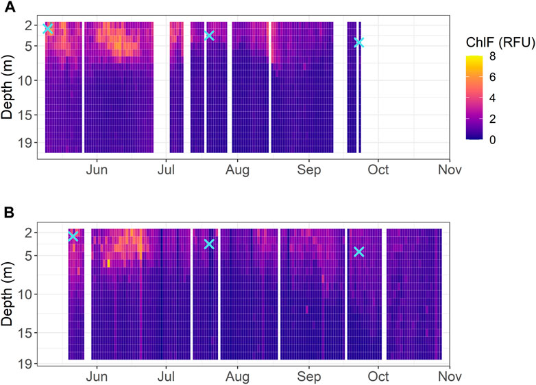
FIGURE 7. NPQ corrected ChlF midday profile in Saadjärv in 2018 (A) and in 2019 (B). Crosses denote Z₉₀ (derived from in situ Secchi depth).

With the advancement of sensors and new methods, ways to study phytoplankton are increasing. Here, we inter-compared three types of methods e.g., laboratory, fluorescence and spectral. While each method has its own advantages, the disadvantages should be or can be filled by alternative method included in the comparison. In parallel, research done on estimating full uncertainty budget for different methods would allow the user to estimate the suitability of each method for their application. Growing constellation of EO satellites allow already now global spatiotemporal analyses on lake phytoplankton, which can be complemented by present and future hyperspectral missions, however, the derived data, either used for calibration, validation or decision making, must be analyzed carefully to avoid artefacts due to selected method.

5 Conclusion

C_Chl-a estimation obtained from six different methods complement each other but are not transferable due to method and season-based differences. Our study on optically different lakes showed:

• The consistency was better in large, well-mixed, eutrophic lake (average bias 0.97, MAE 1.28) compared to the clear-water mesotrophic lake (average bias 0.73, MAE 1.97) where the vertical and short-term temporal variability of the C_Chl-a was larger.

• Similar methods resulted in more consistent results (e.g., S2 and S3 over Võrtsjärv), while adding methods or moving towards clearer lake, the consistency decreased.

• In eutrophic Võrtsjärv, both fluorescence and spectral WISPStation data had high impact on the C_Chl-a retrievals during elevated turbidity indicating the need for more frequent calibration (fluorescence) and adaption of C_Chl-a algorithm for different optical conditions.

• The consistency between C_Chl-a derived from above water radiometry (S2, S3, WISPStation) and fluorescence tended to decrease during high flux intensities in summer (especially in clear water lake) and during low flux intensities in autumn.

• The inherent differences in the methods affect the consistency of C_Chl-a retrievals and might therefore result in seasonal or spatial bias.

Perspectives for future studies include analysis of AHFM fluorescence data, focusing on extrapolation method of integral measurements, effect of frequent calibration and different corrections (e.g., removal of the influence of CDOM and non-algal particles to ChlF) to further investigate the intra-day variability and utilize possibilities by various new hyperspectral sensors (e.g., absorption and scattering features, shift of peaks).

Data availability statement

The raw data supporting the conclusions of this article will be made available by the authors, without undue reservation.

Author contributions

KA, KK, K-LK, and AL contributed to conception and design of the study, KA and K-LK performed data analyses and image processing, KK, AL, MT, and RF contributed with in situ and in vitro data acquisition, KA wrote the main draft of the manuscript, KK and K-LK wrote sections of the manuscript. All authors contributed to manuscript revision, read, and approved the submitted version.

Funding

This research was funded by EU’s Horizon 2020 research and innovation programme (grant agreement no. 730066, EOMORES; grant agreement no. 101004186, Water-ForCE), Estonian Research Council grants PSG10, PSG32, PRG709 and PUTJD913.

Acknowledgments

Authors thank Water Insight for the WISPStation, Centre for Limnology for providing in situ C_Chl-a data for Võrtsjärv. We thank ESA/Copernicus for S2 and S3 images and Estonian Land Board for the possibility to use ESTHub for image processing. We would like to acknowledge four reviewers for valuable comments and suggestions that helped improve this study.

Conflict of interest

The authors declare that the research was conducted in the absence of any commercial or financial relationships that could be construed as a potential conflict of interest.

Publisher’s note

All claims expressed in this article are solely those of the authors and do not necessarily represent those of their affiliated organizations, or those of the publisher, the editors and the reviewers. Any product that may be evaluated in this article, or claim that may be made by its manufacturer, is not guaranteed or endorsed by the publisher.

Supplementary material

The Supplementary Material for this article can be found online at: https://www.frontiersin.org/articles/10.3389/fenvs.2022.989671/full#supplementary-material

References

Al-Kharusi, E., Tenenbaum, D., Abdi, A., Kutser, T., Karlsson, J., Bergström, A.-K., et al. (2020). Large-scale retrieval of coloured dissolved organic matter in northern lakes using sentinel-2 data. Remote Sens. 12, 157. doi:10.3390/rs12010157

CrossRef Full Text | Google Scholar

Alikas, K., Ansko, I., Vabson, V., Ansper, A., Kangro, K., Uudeberg, K., et al. (2020). Consistency of radiometric satellite data over lakes and coastal waters with local field measurements. Remote Sens. 12, 616. doi:10.3390/rs12040616

CrossRef Full Text | Google Scholar

Alikas, K., Kangro, K., Randoja, R., Philipson, P., Asuküll, E., Pisek, J., et al. (2015). Satellite-based products for monitoring optically complex inland waters in support of EU water Framework directive. Int. J. Remote Sens. 36, 4446–4468. doi:10.1080/01431161.2015.1083630

CrossRef Full Text | Google Scholar

Alikas, K., Kangro, K., and Reinart, A. (2010). Detecting cyanobacterial blooms in large North European lakes using the maximum chlorophyll Index. Oceanologia 52, 237–257. doi:10.5697/OC.52-2.237

CrossRef Full Text | Google Scholar

Alikas, K., Kratzer, S., Noorma, A., Soomets, T., and Paavel, B. (2015). Robust remote sensing algorithms to derive the diffuse attenuation coefficient for lakes and coastal waters: Algorithm for diffuse attenuation coefficient. Limnol. Oceanogr. Methods 13, 402–415. doi:10.1002/lom3.10033

CrossRef Full Text | Google Scholar

Ansper, A., and Alikas, K. (2018). Retrieval of chlorophyll a from sentinel-2 MSI data for the European union water Framework directive reporting purposes. Remote Sens. 11, 64. doi:10.3390/rs11010064

CrossRef Full Text | Google Scholar

Bernát, G., Boross, N., Somogyi, B., Vörös, L., G.-Tóth, L., and Boros, G. (2020). Oligotrophication of lake balaton over a 20-year period and its implications for the relationship between phytoplankton and zooplankton biomass. Hydrobiologia 847, 3999–4013. doi:10.1007/s10750-020-04384-x

CrossRef Full Text | Google Scholar

Binding, C. E., Pizzolato, L., and Zeng, C. (2021). EOLakeWatch, delivering a comprehensive suite of remote sensing algal bloom indices for enhanced monitoring of Canadian eutrophic lakes. Ecol. Indic. 121, 106999. doi:10.1016/j.ecolind.2020.106999

CrossRef Full Text | Google Scholar

Binding, C., Zastepa, A., and Zeng, C. (2018). The impact of phytoplankton community composition on optical properties and satellite observations of the 2017 western lake erie algal bloom. J. Gt. Lakes. Res. 45, 573–586. doi:10.1016/j.jglr.2018.11.015

CrossRef Full Text | Google Scholar

Bonansea, M., Ledesma, M., Bazán, R., Ferral, A., German, A., O’Mill, P., et al. (2019). Evaluating the feasibility of using sentinel-2 imagery for water clarity assessment in a reservoir. J. S. Am. Earth Sci. 95, 102265. doi:10.1016/j.jsames.2019.102265

CrossRef Full Text | Google Scholar

Boyer, J., Kelble, C., Ortner, P., and Rudnick, D. (2009)., 9., S56–S67. doi:10.1016/j.ecolind.2008.11.013Phytoplankton bloom status: Chlorophyll a biomass as an indicator of water quality condition in the southern estuaries of Florida, USA, Ecol. Indic.

CrossRef Full Text | Google Scholar

Brentrup, J., Williamson, C., Colom-Montero, W., Eckert, W., Eyto, E., Grossart, H.-P., et al. (2016). The potential of high-frequency profiling to assess vertical and seasonal patterns of phytoplankton dynamics in lakes: An extension of the plankton ecology group (PEG) model. Inland Waters 6, 565–580. doi:10.5268/IW-6.4.890

CrossRef Full Text | Google Scholar

Bulgarelli, B., and Zibordi, G. (2018). On the detectability of adjacency effects in ocean color remote sensing of mid-latitude coastal environments by SeaWiFS, MODIS-A, MERIS, OLCI, OLI and MSI. Remote Sens.Environ 209, 423–438. doi:10.1016/j.rse.2017.12.021

PubMed Abstract | CrossRef Full Text | Google Scholar

Carberry, L., Roesler, C., and Drapeau, S. (2019). Correcting in situ chlorophyll fluorescence time series observations for non-photochemical quenching and tidal variability reveals non-conservative phytoplankton variability in coastal waters. Limnol. Oceanogr. Methods 17, 462–473. doi:10.1002/lom3.10325

PubMed Abstract | CrossRef Full Text | Google Scholar

Cremella, B., Huot, Y., and Bonilla, S. (2018). Interpretation of total phytoplankton and cyanobacteria fluorescence from cross-calibrated fluorometers, including sensitivity to turbidity and colored dissolved organic matter. Limnol. Oceanogr. Methods 16, 881–894. doi:10.1002/lom3.10290

CrossRef Full Text | Google Scholar

Cremona, F., Laas, A., Nõges, P., and Noges, T. (2016). An estimation of diel metabolic rates of eight limnological archetypes from Estonia using high-frequency measurements. Inland Waters 6, 352–363. doi:10.1080/iw-6.3.971

CrossRef Full Text | Google Scholar

Drinkwater, M., and Rebhan, H. (2007). Sentinel-3: Mission requirements document (MRD). ESA, EOP-SMO/1151/MD-md https://earth.esa.int/eogateway/documents/20142/1564943/Sentinel-3-Mission-Requirements-Document-MRD.pdf (Accessed September 7, 2022). 2, 19-22.

Google Scholar

ESTHub (2022). ESTHub satellite data portal. Available at: https://ehdatahub.maaamet.ee/dhus/#/home (Accessed March 15, 2021).

Google Scholar

EUMETSAT (2019). Recommendations for sentinel-3 OLCI ocean Colour product validations in comparison with in situ measurements – matchup protocols. https://www-cdn.eumetsat.int/files/2021-05/Recommendations%20for%20Sentinel-3%20OLCI%20Ocean%20Colour%20product%20validations%20in%20comparison%20with%20in%20situ%20measurements%20%E2%80%93%20Matchup%20Protocols_v7.pdf (Accessed April 12, 2021).

Google Scholar

European Commission (2000). Directive 2000/60/EC of the European parliament and of the Council of 23 october 2000 establishing a Framework for community action in the field of water policy 2000. http://eur-lex.europa.eu/LexUriServ/LexUriServ.do?uri=CELEX:32000L0060:en:NOT (Accessed December 22, 2000).

Google Scholar

European Commission (2008). Directive 2008/56/EC of the European parliament and of the Council of 17 June 2008 establishing a Framework for community action in the field of marine environmental policy 2008. http://eur-lex.europa.eu/LexUriServ/LexUriServ.do?uri=CELEX:32008L0056:en:NOT (Accessed June 25, 2008).

Google Scholar

Fenchel, T. (1988). Marine plankton food chains. Annu. Rev. Ecol. Syst. 19, 19–38. doi:10.1146/annurev.es.19.110188.000315

CrossRef Full Text | Google Scholar

Ferreira, J. G., Andersen, J. H., Borja, A., Bricker, S. B., Camp, J., Cardoso da Silva, M., et al. (2011). Overview of eutrophication indicators to assess environmental status within the European marine Strategy Framework directive. Estuar. Coast. Shelf Sci. 93, 117–131. doi:10.1016/j.ecss.2011.03.014(

CrossRef Full Text | Google Scholar

Ferreira, R. D., Barbosa, C. C. F., and Novo, E. M. L. de M. (2012). Assessment of in vivo fluorescence method for chlorophyll-a estimation in optically complex waters (curuai floodplain, pará - Brazil). Acta Limnol. Bras. 24, 373–386. doi:10.1590/S2179-975X2013005000011

CrossRef Full Text | Google Scholar

Gilerson, A. A., Gitelson, A. A., Zhou, J., Gurlin, D., Moses, W., Ioannou, I., et al. (2010). Algorithms for remote estimation of chlorophyll-a in coastal and inland waters using red and near infrared bands. Opt. Express 18, 24109. doi:10.1364/OE.18.024109

PubMed Abstract | CrossRef Full Text | Google Scholar

Gilerson, A., Zhou, J., Hlaing, S., Ioannou, I., Gross, B., Moshary, F., et al. (2008). Fluorescence component in the reflectance spectra from coastal waters. II. Performance of retrieval algorithms. Opt. Express 16, 2446. doi:10.1364/OE.16.002446

PubMed Abstract | CrossRef Full Text | Google Scholar

Gitelson, A. A., Schalles, J. F., and Hladik, C. M. (2007). Remote chlorophyll-a retrieval in turbid, productive estuaries: Chesapeake bay case study. Remote Sens.Environ. 109, 464–472. doi:10.1016/j.rse.2007.01.016

CrossRef Full Text | Google Scholar

Gittings, J. A., Raitsos, D. E., Racault, M.-F., Brewin, R. J. W., Pradhan, Y., Sathyendranath, S., et al. (2017). Seasonal phytoplankton blooms in the gulf of aden revealed by remote sensing. Remote Sens.Environ. 189, 56–66. doi:10.1016/j.rse.2016.10.043

CrossRef Full Text | Google Scholar

Goldman, E., Smith, E., and Richardson, T. (2013). Estimation of chromophoric dissolved organic matter (CDOM) and photosynthetic activity of estuarine phytoplankton using a multiple-fixed-wavelength spectral fluorometer. Water Res. 47, 1616–1630. doi:10.1016/j.watres.2012.12.023

PubMed Abstract | CrossRef Full Text | Google Scholar

Gons, H. (1999). Optical teledetection of chlorophyll a in turbid inland waters. Environ. Sci. Technol. 33, 1127–1132. doi:10.1021/ES9809657

CrossRef Full Text | Google Scholar

Gower, J., King, S., and Goncalves, P. (2008). Global monitoring of plankton blooms using MERIS MCI. Int. J. Remote Sens. 29, 6209–6216. doi:10.1080/01431160802178110

CrossRef Full Text | Google Scholar

Guan, Q., Feng, L., Hou, X., Schurgers, G., Zheng, Y., and Tang, J. (2020). Eutrophication changes in fifty large lakes on the yangtze plain of China derived from MERIS and OLCI observations. Remote Sens. Environ. 246, 111890. doi:10.1016/j.rse.2020.111890

CrossRef Full Text | Google Scholar

Guinder, V., and Molinero, J. C. (2013). “Climate change effects on marine phytoplankton,” in Marine ecology in a changing world (Boca Raton, FL, USA: CRC Press). ISBN 978-1-4665-9007-6.

Google Scholar

Hama, T., Inoue, T., Suzuki, R., Kashiwazaki, H., Wada, S., Sasano, D., et al. (2015). Response of a phytoplankton community to nutrient addition under different CO2 and PH conditions. J. Oceanogr. 72, 207–223. doi:10.1007/s10872-015-0322-4

CrossRef Full Text | Google Scholar

HELCOM (2006). “Manual for marine monitoring in the COMBINE programme of HELCOM. Part C,” in Programme for monitoring of eutrophication and its effects (Helsinki, Finland, Europe: HELCOM).

Google Scholar

HITACHI (2020). Hitachi instruction manual for model U-3900/3933H spectrophotometer (maintenance manual). Tokyo, Japan: Hitachi High-Tech Science Corporation. 2J2-9011-014 Ver15.

Google Scholar

Hu, C., Feng, L., Lee, Z., Franz, B., Bailey, S., Werdell, J., et al. (2019). Improving satellite global chlorophyll a data products through algorithm refinement and data recovery. J. Geophys. Res. Oceans 124, 1524–1543. doi:10.1029/2019JC014941

CrossRef Full Text | Google Scholar

Järvet, A., and Nõges, P. (1998). Research area and period of L.Võrtsjärv. In Present state and future fate of Lake Võrtsjärv. Tampere 13–22.

PubMed Abstract | Google Scholar

Jeffrey, S. W., and Humphrey, G. F. (1975). New spectrophotometric equations for determining chlorophylls a, b, C1 and C2 in higher plants, algae and natural phytoplankton. Biochem. Physiol. Pflanz. 167, 191–194. doi:10.1016/S0015-3796(17)30778-3

CrossRef Full Text | Google Scholar

Kiselev, V., Bulgarelli, B., and Heege, T. (2014). Sensor independent adjacency correction algorithm for coastal and inland water systems. Remote Sens.Environ 157, 85–95. doi:10.1016/j.rse.2014.07.025

CrossRef Full Text | Google Scholar

Koenings, J. P., and Edmundson, J. A. (1991). Secchi disk and photometer estimates of light regimes in alaskan lakes: Effects of Yellow color and turbidity. Limnol. Oceanogr. 36, 91–105. doi:10.4319/lo.1991.36.1.0091

CrossRef Full Text | Google Scholar

Kromkamp, J., Dijkman, N., Peene, J., Simis, S., and Gons, H. (2008). Estimating phytoplankton primary production in Lake IJsselmeer (The Netherlands) using variable fluorescence (PAM-FRRF) and C-uptake techniques. Eur. J. Phycol. 43, 327–344. doi:10.1080/09670260802080895

CrossRef Full Text | Google Scholar

Kuha, J., Järvinen, M., Salmi, P., and Karjalainen, J. (2020). Calibration of in situ chlorophyll fluorometers for organic matter. Hydrobiologia 847, 4377–4387. doi:10.1007/s10750-019-04086-z

CrossRef Full Text | Google Scholar

Laas, A., Eyto, E., Pierson, D., and Jennings, E. (2016). “NETLAKE guidelines for automatic monitoring station development,”. Technical Report (NETLAKE).

Google Scholar

Longhurst, A., Sathyendranath, S., Platt, T., and Caverhill, C. (1995). An estimate of global primary production in the ocean from satellite radiometer data. J. Plankton Res. 17, 1245–1271. doi:10.1093/plankt/17.6.1245

CrossRef Full Text | Google Scholar

Lorenzen, C. J. (1967). Determination of chlorophyll and pheo-pigments: Spectrophotometric equations. Limnol. Oceanogr. 12, 343–346. doi:10.4319/lo.1967.12.2.0343

CrossRef Full Text | Google Scholar

Luhtala, H., and Tolvanen, H. (2013). Optimizing the use of Secchi depth as a proxy for euphotic depth in coastal waters: An empirical study from the baltic sea. ISPRS Int. J. Geoinf. 2, 1153–1168. doi:10.3390/ijgi2041153

CrossRef Full Text | Google Scholar

Marcé, R., George, G., Buscarinu, P., Deidda, M., Dunalska, J., Eyto, E., et al. (2016). Automatic high frequency monitoring for improved lake and reservoir management. Environ. Sci. Technol. 50, 10780–10794. doi:10.1021/acs.est.6b01604

PubMed Abstract | CrossRef Full Text | Google Scholar

Matthews, M., Bernard, S., and Robertson Lain, L. (2012). An algorithm for detecting trophic status (Chlorophyll-a), cyanobacterial-dominance, surface scums and floating vegetation in inland and coastal waters. Remote Sens. Environ. 124, 637–652. doi:10.1016/j.rse.2012.05.032

CrossRef Full Text | Google Scholar

Matthews, M. W. (2014). Eutrophication and cyanobacterial blooms in South African inland waters: 10years of MERIS observations. Remote Sens. Environ. 155, 161–177. doi:10.1016/j.rse.2014.08.010

CrossRef Full Text | Google Scholar

McKee, D., Cunningham, A., Wright, D., and Hay, L. (2007). Potential impacts of nonalgal materials on water-leaving sun induced chlorophyll fluorescence signals in coastal waters. Appl. Opt. 46, 7720–7729. doi:10.1364/AO.46.007720

PubMed Abstract | CrossRef Full Text | Google Scholar

Meinson, P. (2017). PhD thesis. Tartu, Estonia: Estonian University of Life Sciences.High-frequency measurements – A new approach in limnology

Google Scholar

Meinson, P., Idrizaj, A., Nõges, P., Noges, T., and Laas, A. (2016). Continuous and high-frequency measurements in limnology: History, applications and future challenges. Environ. Rev. 24, 52–62. doi:10.1139/er-2015-0030

CrossRef Full Text | Google Scholar

Meyns, S., Illi, R., and Ribi, B. (1994). Comparison of chlorophyll-a analysis by HPLC and spectrophotometry: Where do the differences come from? Arch. für Hydrobiol. 132, 129–139. doi:10.1127/archiv-hydrobiol/132/1994/129

CrossRef Full Text | Google Scholar

Mograne, M. A., Jamet, C., Loisel, H., Vantrepotte, V., Mériaux, X., and Cauvin, A. (2019). Evaluation of five atmospheric correction algorithms over French optically-complex waters for the sentinel-3a olci ocean color sensor. Remote Sens. 11 (6), 668. doi:10.3390/rs11060668

CrossRef Full Text | Google Scholar

Moiseeva, N., Churilova, T., Efimova, T., and Matorin, D. (2020). Correction of the chlorophyll a fluorescence quenching in the sea upper mixed layer: Development of the algorithm. Phys. Oceanogr. 27, 60–68. doi:10.22449/1573-160X-2020-1-60-68

CrossRef Full Text | Google Scholar

OSPAR Commission (2009). Evaluation of the OSPAR system of ecological quality objectives for the North sea, 102.

Google Scholar

Page, B. P., Olmanson, L. G., and Mishra, D. R. (2019). A harmonized image processing workflow using sentinel-2/MSI and landsat-8/OLI for mapping water clarity in optically variable lake systems. Remote Sens. Environ. 231, 111284. doi:10.1016/j.rse.2019.111284

CrossRef Full Text | Google Scholar

Pahlevan, N., Sarkar, S., Franz, B., V Balasubramanian, S., and He, J. (2017). Sentinel-2 MultiSpectral instrument (MSI) data processing for aquatic science applications: Demonstrations and validations. Remote Sens. Environ. 201, 47–56. doi:10.1016/j.rse.2017.08.033

CrossRef Full Text | Google Scholar

Pahlevan, N., Smith, B., Schalles, J., Binding, C., Cao, Z., Ma, R., et al. (2020). Seamless retrievals of chlorophyll-a from sentinel-2 (MSI) and sentinel-3 (OLCI) in inland and coastal waters: A machine-learning approach. Remote Sens. Environ. 240, 111604. doi:10.1016/j.rse.2019.111604

CrossRef Full Text | Google Scholar

Pereira-Sandoval, M., Ruescas, A., Urrego, P., Ruiz-Verdú, A., Delegido, J., Tenjo, C., et al. (2019). Evaluation of atmospheric correction algorithms over Spanish inland waters for sentinel-2 multi spectral imagery data. Remote Sens. 11 (12), 1469. doi:10.3390/rs11121469

CrossRef Full Text | Google Scholar

Peters, S., Laanen, M., Groetsch, P., Ghezehegn, S., Poser, K., Hommersom, A., et al. (2018). Wispstation: A new autonomous abowe water radiometer system, conference. Dubrovnik: Ocean Optics.

Google Scholar

Picazo, A., Rochera Cordellat, C., Vicente, E., Miracle, M., and Camacho, A. (2013). Spectrophotometric methods for the determination of photosynthetic pigments in stratified lakes: A critical analysis based on comparisons with HPLC determinations in a model lake. Limnetica 32, 139–158. doi:10.23818/limn.32.13

CrossRef Full Text | Google Scholar

Proctor, C., and Roesler, C. (2010). New insights on obtaining phytoplankton concentration and composition from in situ multispectral chlorophyll fluorescence. Limnol. Oceanogr. Methods 8, 695–708. doi:10.4319/lom.2010.8.695

CrossRef Full Text | Google Scholar

Reinart, A., and Kutser, T. (2006). Comparison of different satellite sensors in detecting cyanobacterial bloom events in the baltic sea. Remote Sens. Environ. 102, 74–85. doi:10.1016/j.rse.2006.02.013

CrossRef Full Text | Google Scholar

Reinart, A., and Pedusaar, T. (2008). Reconstruction of the time series of the underwater light climate in a shallow Turbid Lake. Aquat. Ecol. 42, 5–15. doi:10.1007/s10452-006-9056-0

CrossRef Full Text | Google Scholar

Reynolds, C. S. (2006). The ecology of phytoplankton, ecology, biodiversity and conservation. Cambridge, UK: Cambridge University Press.

Google Scholar

Rinke, K., Kuehn, B., Bocaniov, S., Wendt-Potthoff, K., Büttner, O., Tittel, J., et al. (2013). Reservoirs as sentinels of catchments: The rappbode reservoir observatory (harz mountains, Germany). Environ. Earth Sci. 69, 523–536. doi:10.1007/s12665-013-2464-2

CrossRef Full Text | Google Scholar

Ross, J., and Sulev, M. (2000). Sources of errors in measurements of PAR. Agric. For. Meteorol. 100, 103–125. doi:10.1016/S0168-1923(99)00144-6

CrossRef Full Text | Google Scholar

Ruban, A. V. (2016). Nonphotochemical chlorophyll fluorescence quenching: Mechanism and effectiveness in protecting plants from photodamage. Plant Physiol. 170, 1903–1916. doi:10.1104/pp.15.01935

PubMed Abstract | CrossRef Full Text | Google Scholar

Rusak, J., Tanentzap, A., Klug, J., Rose, K., Hendricks, S., Jennings, E., et al. (2018). Wind and trophic status explain within and among-lake variability of algal biomass: Variability of phytoplankton biomass. Limnol. Oceanogr. Lett. 3, 409–418. doi:10.1002/lol2.10093

CrossRef Full Text | Google Scholar

Russak, V., and Kallis, A. (2003). Eesti kiirguskliima teatmik oü stilett trükikoda. Tallinn, Estonia, Europe: Eesti meteoroloogia ja Hüdroloogia Instituut.

Google Scholar

Sayers, M. J., Grimm, A. G., Shuchman, R. A., Deines, A. M., Bunnell, D. B., Raymer, Z. B., et al. (2015). A new method to generate a high-resolution global distribution map of lake chlorophyll. Int. J. Remote Sens. 36, 1942–1964. doi:10.1080/01431161.2015.1029099

CrossRef Full Text | Google Scholar

Seegers, B. N., Stumpf, R. P., Schaeffer, B. A., Loftin, K. A., and Werdell, P. J. (2018). Performance metrics for the assessment of satellite data products: An ocean color case study. Opt. Express 26, 7404–7422. doi:10.1364/OE.26.007404

PubMed Abstract | CrossRef Full Text | Google Scholar

Siegel, D. A., Behrenfeld, M. J., Maritorena, S., McClain, C. R., Antoine, D., Bailey, S. W., et al. (2013). Regional to global assessments of phytoplankton dynamics from the SeaWiFS mission. Remote Sens. Environ. 135, 77–91. doi:10.1016/j.rse.2013.03.025

CrossRef Full Text | Google Scholar

Simmons, L. J., Sandgren, C. D., and Berges, J. A. (2016). Problems and pitfalls in using HPLC pigment analysis to distinguish lake Michigan phytoplankton taxa. J. Gt. Lakes. Res. 42, 397–404. doi:10.1016/j.jglr.2015.12.006

CrossRef Full Text | Google Scholar

Snortheim, C. A., Hanson, P. C., McMahon, K. D., Read, J. S., Carey, C. C., and Dugan, H. A. (2017). Meteorological drivers of hypolimnetic anoxia in a eutrophic, North temperate lake. Ecol. Modell. 343, 39–53. doi:10.1016/j.ecolmodel.2016.10.014

CrossRef Full Text | Google Scholar

Sørensen, K., Grung, M., and Röttgers, R. (2007). An intercomparison of in vitro chlorophyll a determinations for MERIS level 2 data validation. Int. J. Remote Sens. 28, 537–554. doi:10.1080/01431160600815533

CrossRef Full Text | Google Scholar

Steinmetz, F., Deschamps, P.-Y., and Ramon, D. (2011). Atmospheric correction in presence of sun glint: Application to MERIS. Opt. Express 19, 9783–9800. doi:10.1364/OE.19.009783

PubMed Abstract | CrossRef Full Text | Google Scholar

Tamm, M., Freiberg, R., Tõnno, I., Nõges, P., and Nõges, T. (2015). Pigment-based chemotaxonomy - a quick alternative to determine algal assemblages in large shallow eutrophic lake? PLOS ONE 10, e0122526. doi:10.1371/journal.pone.0122526

PubMed Abstract | CrossRef Full Text | Google Scholar

Tamm, M. (2019). PhD thesis. Tartu, Estonia: Estonian University of Life Sciences.Pigment-based chemotaxonomy – efficient tool to quantify phytoplankton groups in lakes and coastal sea areas

Google Scholar

Tilstone, G., Miller, P., Brewin, B., and Priede, I. (2014). Enhancement of primary production in the North atlantic outside of the spring bloom, identified by remote sensing of ocean Colour and temperature. Remote Sens. Environ. 146, 77–86. doi:10.1016/j.rse.2013.04.021

CrossRef Full Text | Google Scholar

Toming, K., Kutser, T., Laas, A., Sepp, M., Paavel, B., and Noges, T. (2016). First experiences in mapping LakeWater quality parameters with sentinel-2 MSI imagery. Remote Sens. 8, 640. doi:10.3390/rs8080640

CrossRef Full Text | Google Scholar

Vansteenwegen, D., Ruddick, K., Cattrijsse, A., Vanhellemont, Q., and Beck, M. (2019). The pan-and-tilt hyperspectral radiometer system (PANTHYR) for autonomous satellite validation measurements-prototype design and testing. Remote Sens. 11, 1360. doi:10.3390/rs11111360

CrossRef Full Text | Google Scholar

Vörös, L., and Padisak, J. (1991). Phytoplankton biomass and chlorophyll-a in some shallow lakes in central europe. Hydrobiologia 215, 111–119. doi:10.1007/BF00014715

CrossRef Full Text | Google Scholar

Warren, M. A., Simis, S. G. H., Martinez-Vicente, V., Poser, K., Bresciani, M., Alikas, K., et al. (2019). Assessment of atmospheric correction algorithms for the Sentinel-2A MultiSpectral Imager over coastal and inland waters. Remote Sens. Environ. 225, 267–289. doi:10.1016/j.rse.2019.03.018

CrossRef Full Text | Google Scholar

Winder, M., and Sommer, U. (2012). Phytoplankton response to a changing climate. Hydrobiologia 698, 5–16. doi:10.1007/s10750-012-1149-2

CrossRef Full Text | Google Scholar

Woolway, R. I., Meinson, P., Nõges, P., Jones, I. D., and Laas, A. (2017). Atmospheric stilling leads to prolonged thermal stratification in a large shallow polymictic lake. Clim. Change 141, 759–773. doi:10.1007/s10584-017-1909-0

CrossRef Full Text | Google Scholar

Zeng, C., Zeng, T., Fischer, A. M., and Xu, H. (2017). Fluorescence-based approach to estimate the chlorophyll-A concentration of a phytoplankton bloom in ardley cove (Antarctica). Remote Sens. 9, 210. doi:10.3390/rs9030210

CrossRef Full Text | Google Scholar

Zhang, Y., Liu, M., Qin, B.-Q., Woerd, H., Li, J., and Li, Y. (2009). Modeling remote-sensing reflectance and retrieving chlorphyll-a concentration in extremely turbid case-2 waters (lake taihu, China). IEEE Trans. Geosci. Remote Sens. 47, 1937–1948. doi:10.1109/TGRS.2008.2011892

CrossRef Full Text | Google Scholar