Break point identification and spatiotemporal dynamic evolution of air pollutants: An empirical study from Anhui province, east China

The new modality of inter-regional joint prevention and control is increasingly important to the integrated process of collaborative governance of air pollutants. Therefore, it has become necessary to analyze the degree of interaction among air pollutants within and between cities, master the dynamics of their spatiotemporal distribution and its influencing factors, and diagnose the primary obstacle factors. Long-term data on the concentrations of six air pollutants among 16 cities of Anhui province from 2015 to 2020 were analyzed using harmonic regression, the coupling coordination degree model, the obstacle degree model, the logarithmic mean Divisia index (LMDI), and exploratory spatial data analysis (ESDA). Over all, the annual mean concentrations of five of these pollutants (NO₂, SO₂, CO, PM₁₀, and PM_2.5) decreased to a certain extent over time, whereas O₃ concentrations increased. The biggest decrease was observed in BZ city, where SO₂ decreased by 80.60% (halving time: −2.03 ± 0.02 years), and the biggest increase was observed in CZ city, where O₃ increased by 113.85% (doubling time: 1.74 ± 0.01 years). The O₃ concentrations in most cities reached their break points starting in 2018, but the break points of other air pollutants appeared earlier than that of O₃, mostly before 2018. With the exception of NO₂ and O₃, the halving times of other air pollutants were basically shorter than the doubling times. The high degree of interaction among air pollutants within and between cities contrasted sharply with the low degree of coordination. An analysis of hotspot evolution revealed that particulate matter (PM₁₀ and PM_2.5) migrated to northern Anhui, NO₂ and O₃ agglomerated to central Anhui, and CO eventually gathered in the Wanjiang City Belt. The primary obstacle factors of air pollutants in Anhui were particulate matter, SO₂ and NO₂. The seasonal differences in primary obstacle factors were most evident in 2020: NO₂ dominated in winter (in 10 cities), SO₂ dominated in southern Anhui, and particulate matter dominated in northern and central Anhui in spring. Other seasons were almost entirely dominated by particulate matter. Industrial structure was found to be more effective in reducing industrial carbon emissions, and technological improvement was found to be more advantageous in reducing industrial particulate matter, NOx and SO₂. Finally, the policy implications of these results and suggestions for strengthening the inter-city joint prevention and control of air pollutants are discussed.

Introduction

As a result of China’s ongoing transfer of its economic structure and industrial layouts in an effort to cut overcapacity, the Yangtze River Delta (YRD) has become a new mega-urban agglomeration and a hub for industrial transfer (Hao Li et al., 2017; Wang et al., 2019; Yu et al., 2020; Chen et al., 2022). The YRD accounted for 24.3% of China’s GDP in 2020 (National Bureau of Statistics of China, 2021).

Anhui province can be considered the economic hinterland of the YRD. Its provincial capital Hefei has become one of the YRD’s urban sub-centers, and its Wanjiang City Belt region has been designated a Demonstration Zone for the national industrial transfer strategy. Anhui is home to 16 of the YRD’s 26 cities, along with 68 national air pollution monitoring stations, accounting for nearly 30% of the YRD’s air quality monitoring capacity.

In 2020, Anhui’s air quality excellence rate was 82.9%, lower than the YRD’s rate of 85.2%. Its annual mean concentrations of SO₂, PM₁₀, and PM_2.5 were also higher than those of the YRD (Anhui: 8 μg/m³ SO₂, 61 μg/m³ PM₁₀, and 39 μg/m³ PM_2.5; YRD: 7 μg/m³ SO₂, 56 μg/m³ PM₁₀, and 35 μg/m³ PM_2.5). The other three air quality indicators were almost equal to those of the YRD (29 μg/m³ NO₂, 1.1 μg/m³ CO, and 152 μg/m³ O₃) (Ministry of Ecology and Environment the Peoples Republic of China, 2021). In light of this, we must be aware that the relocation of heavily polluting enterprises from large cities to small and medium-sized cities, as well as the remarkable changes in the distribution pattern of emission sources, pose new challenges to the effective implementation of the inter-regional joint prevention and control of air pollution. Strengthening inter-city joint prevention and control, undertaking targeted measures specific to each city, co-managing, and avoiding partial governance that applies only to individual cities are particularly important in this regard.

The studies that form the existing literature on air pollution have examined many different geographical areas, including YRD, the Pearl River Delta (PRD), the Beijing-Tianjin-Hebei region (BTH), individual cities, and the entire country (Zheng et al., 2009; Gong et al., 2021; Zhou et al., 2021; Deng et al., 2022; Sun et al., 2022). These studies have focused on temporal and spatial distributions (Zheng et al., 2009; Deng et al., 2022; Su et al., 2022; Zhang and Cheng, 2022), composition and source apportionment (Xue et al., 2019; Zhou et al., 2021; Xu et al., 2022), influencing factors and health effects (Geng et al., 2021; Zhao et al., 2022), and air quality and transport models (Sulaymon et al., 2021; Li et al., 2022; Qin et al., 2022), so as to reveal the distribution features, composition forms, transport characteristics, and health risks of air pollutants. The studies on inter-city joint prevention and collaborative governance of air pollutants have the most practical significance. The studies we reviewed made use of a variety of methods, including exploratory spatial data analysis (ESDA) (Mi et al., 2019), community multi-scale air quality models (Qin et al., 2022), nested air quality prediction model systems (Wang et al., 2013), life cycle inventory models (Chang et al., 2016), the long short-term memory neural network technique (Xiang Li et al., 2017), and social network analysis methods (Du et al., 2021). The latter focused more on the interactive characteristics of the static measurement of air pollution, ignoring the dynamic evolution characteristics, as well as the diagnostic analysis of the primary obstacle factors in the tracking of air pollutants. Given the highly complex nature of the inter-regional air pollution joint prevention and control system and its strong focus on timeliness and regionalism, in-depth explorations of scale selection, method application, and mechanism analysis are needed.

Following China’s implementation of the Air Pollution Prevention and Control Action Plan in 2013, the nationwide air quality excellence rate has improved significantly and the PM_2.5 concentration has decreased continuously. This was followed in 2018 by a 3-Year Action Plan designed to fight air pollution in keeping with the constraint targets set out by the 13th Five-Year Plan, further clarify the specific requirements for optimizing the industrial structure, promote technological improvement, and strengthen inter-regional joint prevention and control. Nevertheless, monitoring the concentrations of various air pollutants remains difficult, due to the variation in their break points and halving times (or doubling times) caused by imbalances among cities in terms of economic development levels, industrial structure layouts, and technical improvements. Fortunately, there is a promising method for identifying the break points of various air pollutants: a combination of the harmonic regression method first proposed by Salamova et al. (2016) to examine the temporal trends of six organophosphate esters in the atmospheric particulate of the North American Great Lakes basin, followed by the use of Microsoft Excel’s Solver feature to identify any statistical difference in the annual change rate before and after the break point (Hites, 2019).

More recently, some studies found a marked improvement in PM_2.5 as a constraint indicator (Li et al., 2019), even as a simultaneous increase in O₃ concentration was also noted (Deng et al., 2022). This result might reflect the low coordination degree between air pollutants within and between cities. Therefore, it is essential to comprehensively understand the interaction degree of air pollutants by quantifying the coupling coordination degree of air pollutants within and between cities for feedback policy regulation. The coupling degree is often used to appraise the interrelation between several systems (Bai et al., 2022; Wu et al., 2022), and the coordination degree is a comprehensive evaluation of the whole system (Dong and Li, 2021). For example, prior research has examined the interrelation between resource allocation schemes and ecological–economic–social subsystems (Wu et al., 2022), water resource spatial equilibrium systems (Bai et al., 2022), urbanization and atmospheric/terrestrial ecosystems (Liu et al., 2018; Xiao et al., 2020), and socio-economic and infrastructure development (Tomal, 2020) by quantifying the coupling coordination degree. Additionally, the obstacle degree model has been introduced to allow a deeper exploration of the primary factors that constrain the collaborative governance of inter-city air pollution. Xu et al. (2021) diagnosed the primary obstacle factors restricting the sustainable development of cities and their dynamic trends in the YRD. Bai et al. (2022) employed the obstacle degree model to identify the primary obstacle factors in Anhui’s water resource spatial equilibrium system.

The air quality of a city is closely associated with the emission of industrial pollutants (SO₂, NOx, particulate matter, and carbon emissions). Hence, quantifying the contributions to emission reductions made by, e.g., economic growth, technological improvements, industrial structure, and population size may help to reflect accurately the effects of policies targeting industrial pollutant emissions and potentially facilitate more targeted measures. LMDI is a factor decomposition model developed in 1998 on the basis of the index decomposition method (Ang, 2015). This model allows the measurement of changes in the factors corresponding to net effects during any period of time. It does not contain residual terms, thus overcoming the zero-value issue (Ang, 2015). LMDI has been widely used in the carbon emissions (Jing Liu et al., 2022), energy (Lin and Long, 2016), and environmental fields (Geng et al., 2021; Pei et al., 2022). Therefore, the present study employs LMDI models to quantitatively analyze the factors influencing industrial pollution emissions in 16 cities of Anhui.

For the present study, we first determined the temporal trend and break point of air pollutants by combining harmonic regression with the Solver feature of Excel, established a measurement model for the coupling coordination degree of these air pollutants, and quantitatively analyzed the trends in coupling and coordination degree changes within and between the cities of Anhui province. We then diagnosed primary obstacle factors and plotted the spatial dynamic evolution of the air pollutants under study using ESDA. Finally, we explored the driving factors (economic growth, technological improvement, industrial structure, and population size) affecting industrial pollutant emission (SO₂, NOx, particulate matter, and carbon emissions) using LMDI, and we offer relevant suggestions to strengthen inter-city air pollutant joint prevention and control.

Materials and methods

Study area and data sources

A detailed description of the study area is presented in Supplementary Text S1 (see Supplementary Material). The study area is shown in Figure 1.

FIGURE 1

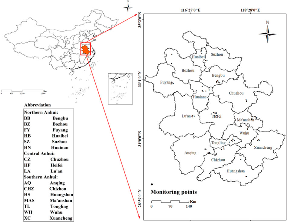
FIGURE 1. A sketch map of the study area.

The daily mean concentration data of six air pollutants were recorded from the real-time air quality release platform (https://sthjt.ah.gov.cn/) of Anhui province’s Department of Ecology and Environment. (CO was measured in mg/m³, and the other five air pollutants were measured in μg/m³.) Data between 1 January 2015 and 31 December 2020 were collected. Each year was divided into four seasons: spring (March to May), summer (June to August), autumn (September to November), and winter (December to February of the following year). The population, industrial GDP and overall GDP data of each city in Anhui, and industrial pollution emission levels (NOx, SO₂, and particulate matter) were recorded from the Anhui Statistical Yearbook (http://tjj.ah.gov.cn/).

Break point identification and prediction approach

The six air pollutants’ inter-annual variation trends were studied using the harmonic regression equation. First, the concentration data for the six pollutants were converted into the corresponding natural logarithm concentration data, and then the relationship between concentration and time was plotted using Eq. 1 (Salamova et al., 2016).

$\ln \left(C_t\right)=a_{\mathit{0}}+a_{\mathit{1}}\mathit{sin}\left(zt\right)+a_{\mathit{2}}\mathit{cos}\left(zt\right)+a_{\mathit{3}}t(1)$

where C_t is the observed concentration of air pollutants at time t; and z = 2π/365.25, which sets 1 year as a periodic cycle. The value range of t starts from the calendar day 1 January 2015. The intercept is $a_{\mathit{0}}$; $a_{\mathit{1}}$ and $a_{\mathit{2}}$ are harmonic coefficients; and $a_{\mathit{3}}$ is the first-order rate constant, which can be used to calculate the halving time [$t_{\mathit{1}/\mathit{2}}=-\ln \left(2\right)/\left(365.25a_{\mathit{3}}\right)$] and doubling time [${\mathrm{t}}_2=\ln \left(2\right)/\left(365.25a_{\mathit{3}}\right)$] of air pollutants.

For this study, we simplified the break point identification approach established by Hites (2019) into the following steps: Step 1 Determine break points. In combination with the trends in the annual mean concentrations of each air pollutant, annual mean concentration variation trend of air pollutants (Supplementary Figure S1), a significant increase or decrease was observed before or after a certain point. Step 2 Identify break points. As shown in Eq. 2, Microsoft Excel’s Solver feature was used to calculate SR_min values before and after the break point to make the determined break point more objective.

${SR}_{\mathit{min}}=\sum {\left[\ln \left(C_t\right)-\widehat{\ln \left(C_t\right)}\right]}^2(2)$

where $\widehat{\ln \left(C_t\right)}$ is the predicted concentration of air pollutants at time t. The minimum value of SR was fixed via the Solver feature to automatically match the values of $a_{\mathit{0}}$, $a_{\mathit{1}}$, $a_{\mathit{2}}$ , and $a_{\mathit{3}}$. Step 3 Validate break points. The t-test was used for break point validations depending on a statistically significant difference between the doubling and halving times.

The coupling coordination degree and obstacle degree models

The coupling degree can be used to evaluate the interaction and influence of two or more socio-economic systems. On this basis, a method for analyzing the coupling coordination degree was developed as a way to judge the degree of coordinated development between each system. In this study, the coupling coordination degree was used to reflect the intra-city interactions and level of coordinated development among the six air pollutants. The air quality index (AQI) was also used to measure the coupling coordination degree and to reflect the six pollutants’ inter-city interactions and levels of coordinated development. For more details on the calculation of AQI, please refer to our previous work (Xue et al., 2019).

The calculation and related equations for the coupling coordination degree were as follows:

Step 1. The coefficient of variation method was used to objectively weight air pollutants within each city, as well as the AQI between cities. As shown in Eqs 3, 4, the objectivity of this weighting method was based on the differences within the data samples, rather than on the theoretical importance of specific indicators.

${\mathit{C}\mathit{V}}_{\mathit{i}\mathit{j}}=\frac{{\mathit{\delta }}_{\mathit{i}\mathit{j}}}{{\overline{\mathit{A}}}_{\mathit{i}\mathit{j}}}(3)$

${\mathit{W}}_{\mathit{i}\mathit{j}}=\frac{{\mathit{C}\mathit{V}}_{\mathit{i}\mathit{j}}}{{\displaystyle \sum }_{\mathit{j}=\mathit{1}}^{\mathit{n}}{\mathit{C}\mathit{V}}_{\mathit{i}\mathit{j}}}(4)$

Where ${CV}_{ij}$ denotes the coefficient of variation; $W_{ij}$ denotes weight; ${\delta }_{ij}$ denotes the standard deviation of the j-th indicator in the i-th city; and ${\overline{A}}_{ij}$ denotes the mean value of the j-th indicator in the i-th city. Note that, where the six air pollutants were replaced by AQI as the measurement indicators, the corresponding i and j denoted the i-th region (such as northern Anhui, central Anhui, or southern Anhui) and the j-th city, respectively.

Step 2. The coupling coordination degree, as a non-dimensional parameter, should be calculated using data converted from the corresponding indicators; otherwise, these data cannot be added. Here, the extremum method was employed for data standardization (see Eq. 5), and then the standardized value was put into Eq. 6 to obtain the corresponding individual index for each air pollutant. These indices were then incorporated into Eq. 7 to obtain the coupling degree. Following that, the coordination index was obtained by using Eq. 8, which allowed the coordination degree to be obtained by calculating the square root of the product of the coupling degree and the coordination index (see Eq. 9).

${\mathit{A}}_{\mathit{i}\mathit{j}}^{\prime }=\frac{{\mathit{A}}_{\mathit{i}\mathit{j}}-{\mathit{Min}}_{\mathit{i}\mathit{j}}}{{\mathit{Max}}_{\mathit{i}\mathit{j}}-{\mathit{Min}}_{\mathit{i}\mathit{j}}}(5)$

${\mathit{A}\mathit{I}}_{\mathit{i}\mathit{j}}=\frac{{\mathit{W}}_{\mathit{i}\mathit{j}}{\displaystyle \sum }_{\mathit{j}=\mathit{1}}^{\mathit{n}}{\mathit{A}}_{\mathit{i}\mathit{j}}^{\prime }}{\mathit{n}}(6)$

$\mathit{C}=\frac{{\left({\displaystyle \mathit{\prod }}_{\mathit{j}=\mathit{1}}^{\mathit{n}}{\mathit{A}\mathit{I}}_{\mathit{i}\mathit{j}}\right)}^{\frac{\mathit{1}}{\mathit{n}}}}{\frac{{\displaystyle \mathit{\sum }}_{\mathit{j}=\mathit{1}}^{\mathit{n}}{\mathit{A}\mathit{I}}_{\mathit{i}\mathit{j}}}{\mathit{n}}},\mathit{C}\in \left[\mathbf{0},\mathbf{1}\right](7)$

$\mathit{T}={\displaystyle \mathit{\sum }}_{\mathit{j}=\mathit{1}}^{\mathit{n}}\left({{\mathit{W}}_{\mathit{i}\mathit{j}}\times \mathit{A}\mathit{I}}_{\mathit{i}\mathit{j}}\right)(8)$

$\mathit{D}=\sqrt{\mathit{C}\times \mathit{T}}(9)$

where $A_{ij}^{\prime }$ is $A_{{NO}_{\mathit{2}}}^{\prime }$, $A_{{SO}_{\mathit{2}}}^{\prime }$, $A_{CO}^{\prime }$, $A_{O_{\mathit{3}}}^{\prime }$, $A_{{PM}_{\mathit{10}}}^{\prime }$, and $A_{{PM}_{\mathit{2.5}}}^{\prime }$ (or $A_{AQI}^{\prime }$) in the i-th city, denoting the corresponding standardized values. The variables $A_{ij}$, ${\mathit{Max}}_{ij}$, and ${\mathit{Min}}_{ij}$ denote the corresponding concentration and the maximum and minimum values of NO₂, SO₂, CO, O₃, PM₁₀, and PM_2.5 (or maximum and minimum values of AQI), respectively. ${AI}_{ij}$is ${AI}_{{NO}_{\mathit{2}}}$, ${AI}_{{SO}_{\mathit{2}}}$,${AI}_{CO}$ , ${AI}_{O_{\mathit{3}}}$, ${AI}_{{PM}_{\mathit{10}}}$ , and ${AI}_{{PM}_{\mathit{2.5}}}$ (or ${AI}_{AQI}$) in the i-th city, denoting the corresponding individual index. C denotes the coupling degree, and the value of the function is between 0 and 1. The greater the C, the higher the coupling degree, indicating that the dispersion degree between ${AI}_{{NO}_{\mathit{2}}}$, ${AI}_{{SO}_{\mathit{2}}}$,${AI}_{CO}$, ${AI}_{O_{\mathit{3}}}$, ${AI}_{{PM}_{\mathit{10}}}$ , and ${AI}_{{PM}_{\mathit{2.5}}}$ (or ${AI}_{AQI}$) is smaller, which can better reflect the interaction degree between air pollutants and effectively avoid a zero-value issue.In addition, the division standard of the coupling degree is an important basis for determining the degree of interaction between target objects. Cong (2019) found that the existing two kinds of coupling models were of zero-order homogeneity, and that when there were more than three targeting objects (n ≥ 3), two measurement results had differences in overestimates or underestimates. Therefore, dividing the coupling degree interval was largely subjective. Cong (2019) suggested that the standard interval should be established based on target objects and the coupling degree measurement approach. Dong and Li (2021) divided the coupling degree interval according to the coupling degree measurement results in their research on the up-middle-downstream relationships of China’s wind power industrial chain. T denotes the coordination index, reflecting the contribution of the air pollutants within a city (or the inter-city AQI) to the coordination degree. In this study, the coupling degree interval was divided into seven grades according to the coupling degree measurement results in different seasons; the coordination degree interval was divided into 10 grades (Supplementary Table S1) (Dong and Li, 2021).

Step 3. The primary obstacle factors were analyzed and diagnosed using the factor contribution degree, index deviation degree, and obstacle degree. The factor contribution degree was measured using the weight of the individual indicators. The index deviation degree denoted the gap between the individual indicators and the environmental air quality of the city, that is, the gap between the standardized value of the individual indicators and 100%. The obstacle degree denoted the influence degree of the j-th air pollutant in the i-th city. The maximum obstacle degree of the individual indicators was selected in the same criteria layer as the primary obstacle factor. Further, Eqs 10, 11 were used,

${\mathit{U}}_{\mathit{i}\mathit{j}}=\frac{{\mathit{W}}_{\mathit{i}\mathit{j}}\times \left(\mathit{1}-{\mathit{A}}_{\mathit{i}\mathit{j}}^{\prime }\right)}{{\displaystyle \sum }_{\mathit{j}=\mathit{1}}^{\mathit{n}}({\mathit{W}}_{\mathit{i}\mathit{j}}\times \left(\mathit{1}-{\mathit{A}}_{\mathit{i}\mathit{j}}^{\prime }\right))}\times \mathbf{100}\%(10)$

${\mathit{U}}_{\mathit{max}}=\left\{{\mathit{U}}_{\mathit{i}\mathit{j}}\right\}(11)$

where $U_{ij}$ denotes the individual indicator obstacle degree and $U_{\mathit{max}}$ denotes the primary obstacle factors.

Exploratory spatial data analysis

ESDA was used to analyze the spatial pattern of pollutants, which mainly included global spatial autocorrelation and local spatial autocorrelation. An introduction to ESDA methods is provided in Supplementary Text S2.

Index decomposition model

This study selected four indices—technological improvement, industrial structure, economic growth, and population size—and analyzed the influence of each on the emission of industrial air pollution (NOx, SO₂, particulate matter, and carbon). Carbon emissions released by energy consumption in the industrial sector were calculated using the IPCC, 2006 Guidelines for National Greenhouse Gas Inventories provided by the Intergovernmental Panel on Climate Change. The total carbon emission measurement and the decomposition of the LMDI model equation are shown in Supplementary Text S3.

Results

Identification of break points and air pollutants’ inter-annual trends

The inter-annual trends of six air pollutants (NO₂, SO₂, CO, O₃, PM₁₀, and PM_2.5) in Anhui province from 2015 to 2020 are shown in Supplementary Figures S1A–C. After applying the break point identification method, it was found that the break point of NO₂ in central Anhui (CZ, HF, and LA) was 2017, and the halving time (−5.85 ± 0.15 years to −9.19 ± 0.34 years) was about two to three times the doubling time (2.15 ± 0.02 years to 4.48 ± 0.07 years) (Table 1). The observed and predicted values are shown in Supplementary Figure S2A–C. The break points of NO₂ in northern Anhui were concentrated in 2016, and they were located in FY, HB, and HN. The doubling time for HN was 3.10 ± 0.03 years, and the halving time was −34.91 ± 5.32 years, a difference of more than 10 times (Table 1). However, the doubling time and halving time for SZ were 3.86 ± 0.05 years and −3.23 ± 0.05 years, respectively, and its break point was in 2018 (t = 94.82, p < 0.001). The break point of NO₂ in several cities, including AQ, HS, and XC, was in 2016, and the halving time in these cities was about three to seven times the doubling time (Table 1). Three cities along the Yangtze River (MAS, TL, and WH) had consistent break points, all in 2017. The halving time of NO₂ in CHZ was −3.13 ± 0.03 years, which was faster than that of the remaining six cities (AQ, HS, MAS, TL, WH, and XC) in southern Anhui.

TABLE 1

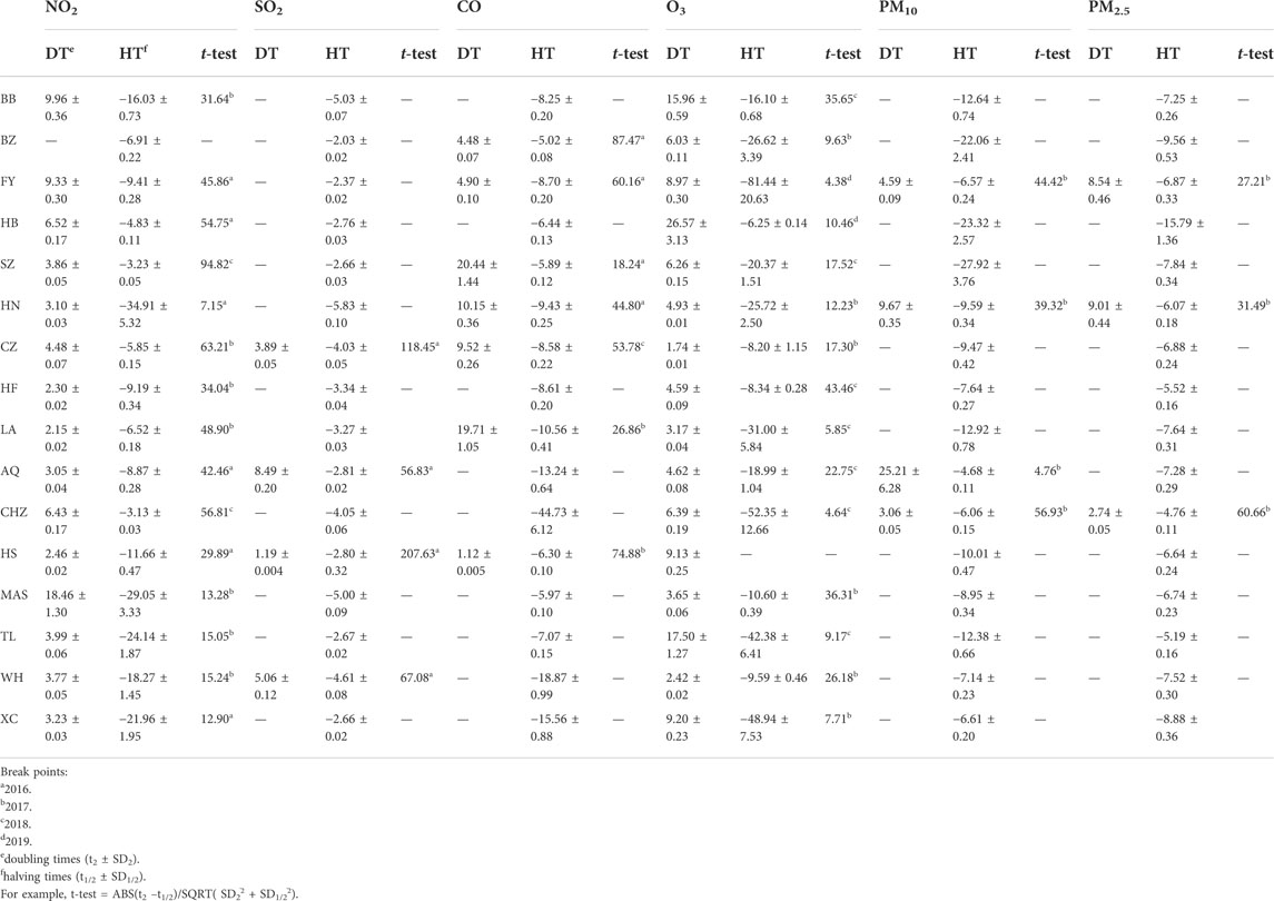
TABLE 1. Halving times (negative numbers) and doubling times (positive numbers) times, in years, for air pollution concentrations in Anhui Province during the period 2015–2020.

Compared with central and southern Anhui, SO₂ in northern Anhui (BB, BZ, FY, HB, SZ, and HN) did not show a break point and continued to decrease (Table 1). The SO₂ halving time was the fastest in BZ, at only −2.03 ± 0.02 years. In four cities (CZ, AQ, HS, and WH), the break point of SO₂ was uniform, occurring in 2016 (Supplementary Figure S1; Table 1). The most significant difference before and after the break point was seen in AQ (t = 56.83, p < 0.001); the halving time (−2.81 ± 0.02 years) was only one third of the doubling time (8.49 ± 0.20 years).

The break points of CO appeared in 2016 (BZ, FY, SZ, and HN), 2017 (LA and HS), and 2018 (CZ), respectively (Table 1). In BZ, the doubling time and halving time of CO were relatively close, with a significant difference before and after the break point (t = 87.47, p < 0.001). In addition, CHZ, as one of several cities that did not show a break point, had a relatively slow CO halving time (−44.73 ± 6.12 years).

Beginning in 2018, most cities had O₃ break points, though northern Anhui lagged behind central and southern Anhui (Table 1). The shortest doubling times of O_3, from north to south, are as follows: 4.93 ± 0.01 years (HN in northern Anhui), 1.74 ± 0.01 years (CZ in middle Anhui), and 2.42 ± 0.02 years (WH in southern Anhui). Each city’s respective halving time, however, was not among the shortest. In BZ, in northern Anhui, O₃ break point appeared relatively early (2017). In HF, in central Anhui, the O₃ break point was delayed to 2018, and its halving time was about −8.34 ± 0.28 years. In southern Anhui, only HS did not show an O₃ break point; its doubling time was 9.13 ± 0.25 years (Table 1).

The average halving time of particulate matter displayed a gradual increase from north to south: −12.96 years in northern Anhui, −8.35 years in central Anhui, and −7.35 years in southern Anhui. PM₁₀ and PM_2.5 showed a break point in a few cities, almost all of which occurred in 2017 (Table 1).

Analysis of the coupling coordination degree of air pollutants

The coupling degree of air pollutants in Anhui from 2015 to 2020 was between 0.890 and 0.985, with a running-in stage in most cities (Table 2). The annual mean coupling degree of air pollutants, from north to south, was 0.963 (0.942–0.985), 0.953 (0.901–0.976), and 0.952 (0.890–0.985), respectively, and the number of cities in the antagonistic stage gradually increased. Furthermore, the analysis of the coupling degree of air pollutants in different seasons revealed that the coupling degree, from high to low, was as follows: spring (0.965), winter (0.960), autumn (0.955), and summer (0.943) (Supplementary Table S3). On balance, the air pollutants in most cities of Anhui were in the running-in stage in spring, winter and autumn, and in the antagonistic stage in summer. It should be pointed out that very few cities had a coupling degree lower than 0.85, a very low level; they are AQ in the winter of 2015, HS and XC in the summer of 2016, and FY in the autumn of 2018 (Supplementary Table S3).

TABLE 2

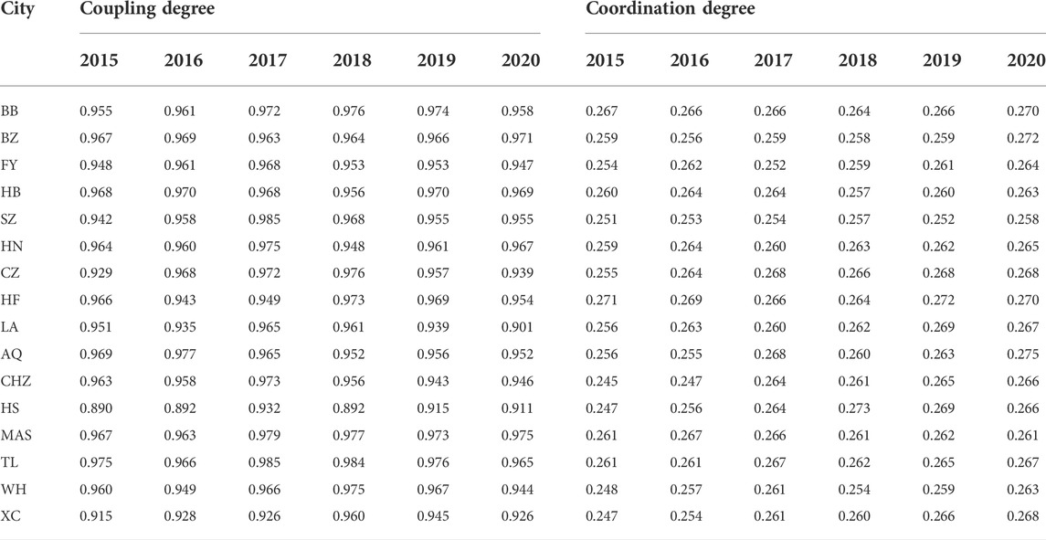
TABLE 2. Coupling and coordination degrees of air pollutants in Anhui province, 2015–2020 between 2015 and 2020.

The annual mean coupling degree measured using AQI was 0.987 (0.966–0.995). The coupling degrees of AQI in spring (0.984) and summer (0.981) were below the mean, while those in autumn (0.990) and winter (0.992) were above the mean (Table 3). As shown in Table 3, the AQI coupling degree had a good-level coupling in spring, summer, and autumn, and a high-level coupling in winter. The coupling degree of AQI in different regions of Anhui is shown in Supplementary Table S4. The mean coupling degrees of AQI in three regions were 0.992 (northern Anhui), 0.994 (central Anhui), and 0.991 (southern Anhui), indicating that they had a high-level coupling.

TABLE 3

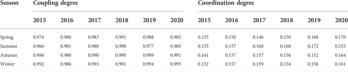
TABLE 3. Coupling and coordination degrees of AQI in Anhui province, 2015–2020.

The coordination degree of air pollutants in Anhui between 2015 and 2020 was in the range of 0.245–0.275, and all cities were in a moderate state of maladjustment (Table 2). The annual mean coordination degrees, arranged from north to south, were 0.260, 0.266, and 0.261, respectively, with the highest value in central Anhui. In addition, the annual mean coordination degree displayed a trend of increasing year over year. The corresponding values for each year were 0.256 (0.245–0.271) in 2015, 0.260 (0.247–0.269) in 2016, 0.263 (0.252–0.268) in 2017, 0.261 (0.254–0.273) in 2018, 0.264 (0.252–0.272) in 2019, and 0.266 (0.258–0.275) in 2020. The seasonal distribution of the air pollutant coordination degree in Anhui is shown in Supplementary Table S3. The seasonal variations in the annual mean coordination degree, arranged from highest to lowest, were summer (0.266), autumn (0.262), winter (0.260), and spring (0.259). At the same time, the annual mean coordination degree showed an ascending trend in all seasons from 2015 to 2020.

The coordination degree range of the AQI was between 0.146 and 0.172, with severe maladjustment (Table 3). The seasonal difference was not significant. The coordination degree of AQI was significantly different between the three regions (Supplementary Table S4), largely caused by the difference between central Anhui and northern and southern Anhui. The coordination degree of AQI among the three cities of central Anhui ranged from 0.341 to 0.409, which was between mild maladjustment and on the verge of maladjustment. Northern and southern Anhui were in moderate maladjustment, and their coordination degrees of AQI were 0.221–0.280 and 0.224–0.268, respectively.

Exploratory spatial data analysis of air pollutants

The global spatial autocorrelation was analyzed based on Global Moran’s I and General G measured using ArcGIS 10.3.1 software. The spatiotemporal evolution characteristics of the hot and cold spots of six air pollutants in Anhui between 2015 and 2020 were measured using the Getis-Ord Gi* formula. According to Global Moran’s I (Table 4), the z-score ranges of air pollutants in Anhui were 79.01–371.51 (2015), 58.53–354.46 (2016), 60.77–273.43 (2017), 60.00–333.50 (2018), 54.71–410.15 (2019), and 26.34–360.81 (2020). Generally, if the z-score is greater than 1.96, it is significant; and if the z-score is greater than 2.58, it is extremely significant. In this study, the z-scores were all greater than 2.58, and the I values were all greater than 0 (the range of I was 0.02–0.38, as shown in Table 4). This indicates that the six air pollutants had a significant positive spatial autocorrelation, namely, that spatial dependence existed. Meanwhile, the p-values of the air pollutants for each year were lower than 0.01 (Table 4), which also indicated a significant spatial agglomeration distribution of air pollutants among the 16 cities of Anhui. In addition, the General G test (Table 4) found that G (d) values in all years were greater than 0, with p-values lower than 0.01. According to this test, the z-score of the six air pollutants ranged from 23.88 to 410.17, indicating a high level of agglomeration. Furthermore, the seasonal division of the results of the two tests (Supplementary Tables S5–S8) indicated that the air pollutants in Anhui showed significant positive spatial autocorrelation and high agglomeration in each season (z-score > 2.58, I ∈ [0.01, 0.64], p < 0.01).

TABLE 4

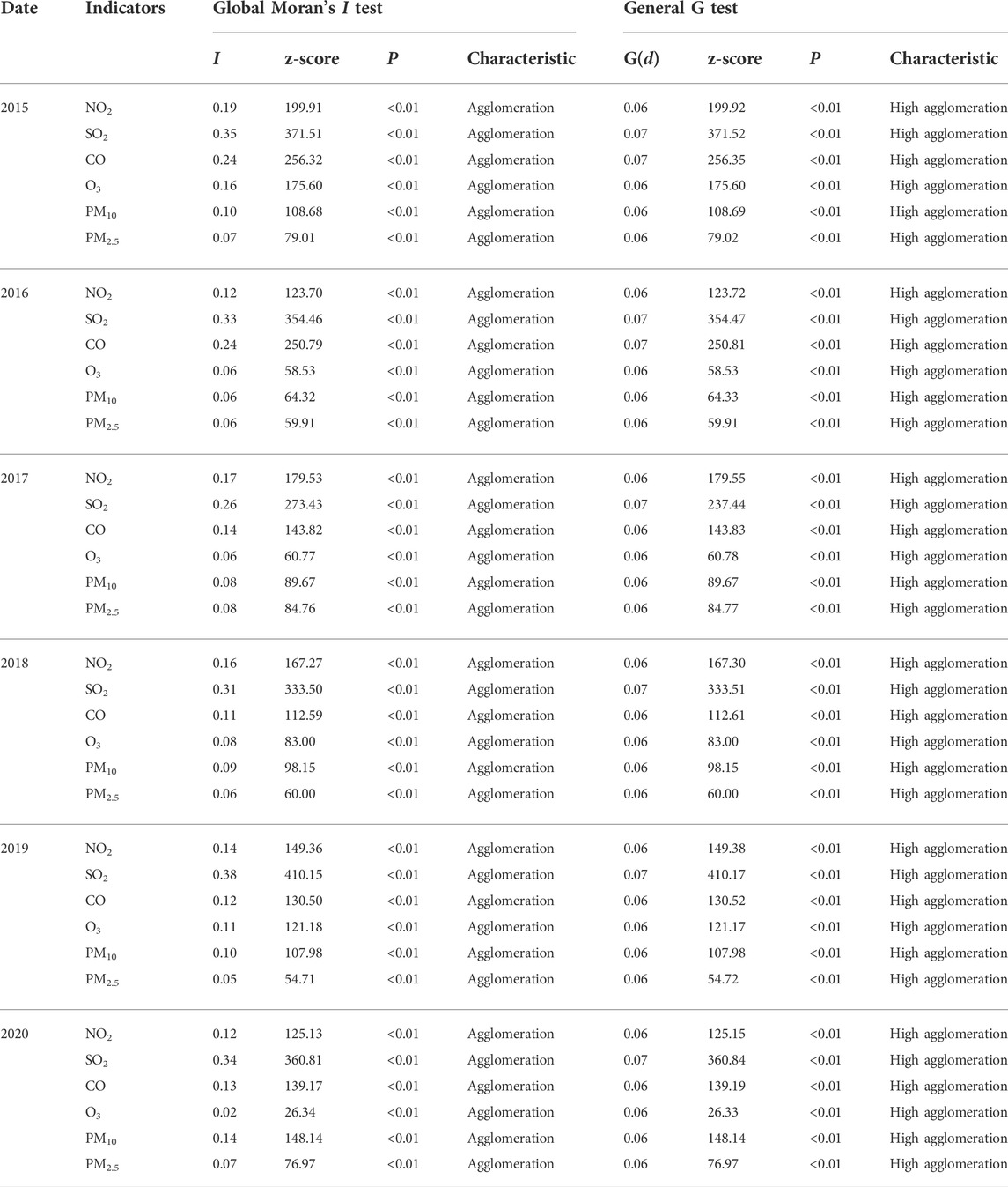
TABLE 4. Global spatial correlation of air pollutants, as calculated via the Moran’s I and General G tests.

On the whole, between 2015 and 2020, the hotspot evolution of six air pollutants in Anhui mainly experienced the following (Figures 2, 3): agglomeration to central Anhui (NO₂ and O₃) and migration to northern Anhui (PM₁₀ and PM_2.5). The NO₂ and O₃ hotspots formed gradually near central Anhui from 2015 to 2020 (Figure 2). The distribution of NO₂ hotspots gradually evolved from BB, BZ, FY, HB, HF, MAS, WH, TL, and XC in 2015 to BB, CZ, HF, MAS, WH, and TL in 2020, with high agglomeration. The number of cold spot cities also increased significantly, with XC city evolving from a hotspot city in 2015 to a not-significant city in 2020 (Figure 2). From the seasonal change point of view, the hotspot evolution of NO₂ showed a trend of agglomeration to central Anhui between 2015 and 2020 (Supplementary Figure S3). In the summer and autumn of 2015, the hotspot distribution of NO₂ was basically the same as that of the whole year, and a hotspot distribution thread ran through Anhui from north to south. Ultimately, across the four seasons of 2020, the NO₂ hotspot distribution extended to the periphery with HF as the center, including CZ, HF, MAS, WH, TL, and others.

FIGURE 2

FIGURE 2. Hotspot evolution of NO₂ and O₃ in Anhui province.

FIGURE 3

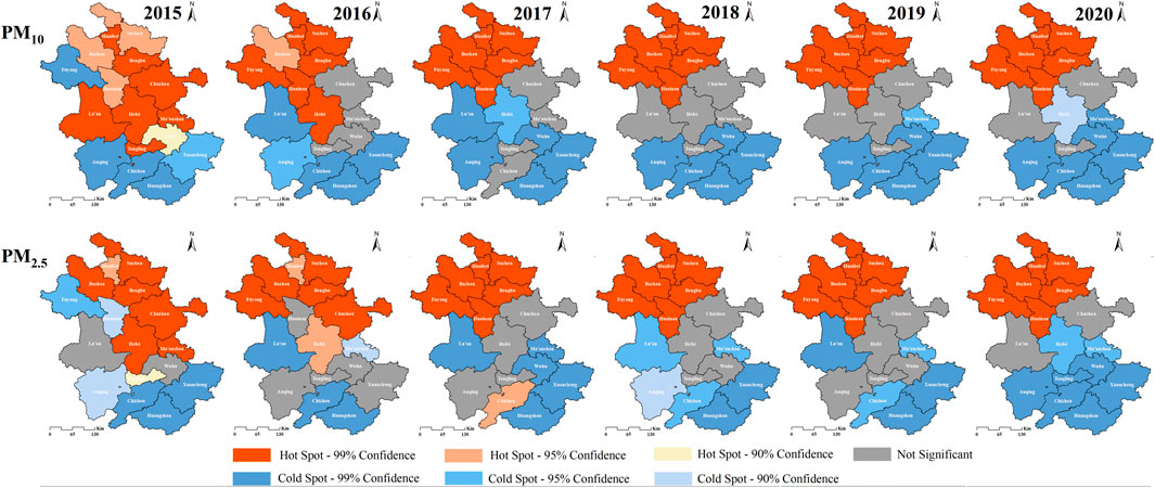
FIGURE 3. Hotspot evolution of PM₁₀ and PM_2.5 in Anhui province.

In 2015, O₃ hotspots were concentrated in northern Anhui (BB, BZ, FY, HB, and SZ) and southern Anhui (CHZ and XC), with not-significant cities including HN, HF, AQ, MAS, and TL; only CZ, LA, HS, and WH were cold spot cities. Until 2018, the number of O₃ hotspot cities increased to 10, covering northern Anhui (BB, BZ, HB, HN, and SZ), central Anhui (CZ and LA), and southern Anhui (AQ, MAS, and WH). However, the hotspot distribution of O₃ in 2020 showed a trend of agglomeration to central Anhui; that is, no hotspot city existed in southern Anhui, one hotspot city was added to central Anhui, and northern Anhui lost two hotspot cities (Figure 2). The hotspot evolution trend of O₃ showed significant seasonal variation (Supplementary Figure S3). Every spring from 2015 to 2019, the number of hotspot cities of O₃ increased gradually from north to south. By spring 2020, the number of hotspot cities had decreased significantly, and most of them had converged in northern Anhui. During the summers of 2015–2020, O₃ hotspots underwent a shift from displaying a north-south distribution to gathering in central Anhui and then extending to northern Anhui. In autumn, O₃ hotspot cities were relatively few and scattered, and by 2020, the only O₃ hotspot cities were CZ and LA. In winter, O₃ hotspot cities were mainly distributed in northern and southern Anhui prior to 2017, and after 2017, most of them were distributed in central and southern Anhui.

As shown in Figure 3, the hotspot evolution trend of PM₁₀ and PM_2.5 demonstrated a significant migration to northern Anhui. In 2015, PM₁₀ hotspots were concentrated in northern Anhui (BB, BZ, HB, HN, and SZ), central Anhui (CZ, HF, and LA), and southern Anhui (MAS, WH, and TL). Subsequently, the hotspot cities in central and southern Anhui gradually transitioned to not-significant cities or cold spot cities between 2016 and 2020, until only a cluster within northern Anhui remained (BB, BZ, FY, HB, HN, and SZ). The cold and hot spot evolution trend of PM_2.5 was basically in line with that of PM₁₀, and the hotspot cities of PM_2.5 were eventually assembled in northern Anhui. The seasonal variation in the hotspot evolution of PM₁₀ and PM_2.5 was roughly consistent (Supplementary Figure S4). PM₁₀ and PM_2.5 hotspot cities were all concentrated significantly in northern Anhui for three seasons of the year, with the exception of summer.

Although the hotspot evolution trend of SO₂ and CO was not clear at first glance, it was found that SO₂ showed a trend of decreasing hotspot cities and increasing cold spot cities year after year, whereas the CO hotspots were eventually concentrated in six of the nine cities in the Wanjiang City Belt (CZ, LA, MAS, WH, TL, and CHZ) (Figure 4). The seasonal variation in the hotspot evolution of SO₂ and CO is shown in Supplementary Figure S5. In spring, SO₂ hotspots kept in step with those of winter; before 2018, SO₂ hotspot cities were mostly concentrated in northern Anhui, but after 2018, they significantly decreased and dispersed. The SO₂ trends in summer and autumn were basically the same; namely, in 2018, SO₂ hotspot cities were mostly distributed in northern and southern Anhui, and after 2018, they also significantly decreased and dispersed. It is worth noting that TL has always been a hotspot city in all seasons. Compared with northern Anhui, central and southern Anhui were more likely to experience a convergence of CO hotspot cities, especially the Wanjiang City Belt, which became a CO hotspot region in all seasons except winter (Supplementary Figure S5).

FIGURE 4

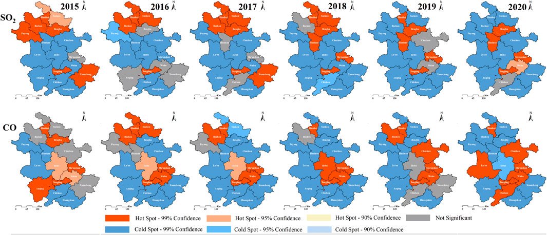
FIGURE 4. Hotspot evolution of SO₂ and CO in Anhui province.

Diagnosis of air pollutant obstacle degrees

The diagnostic results of each air pollutant’s obstacle degree levels during 2015–2020 are shown in Figure 5. We detected year-by-year changes in the air pollutants that became primary obstacle factors: PM_2.5, SO₂, CO, and O₃ (2015); PM_2.5 and PM₁₀ (2016); PM_2.5, PM₁₀, and SO₂ (2017); PM_2.5, PM₁₀, SO₂, and NO₂ (2018 and 2019); and PM_2.5, PM₁₀, and NO₂ (2020).

FIGURE 5

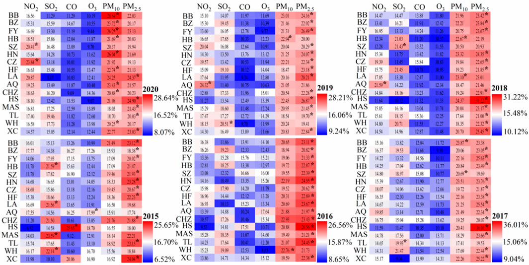
FIGURE 5. Obstacle degree levels of air pollutants in Anhui, 2015–2020. (* = primary obstacle factor).

In 2015, the cities with SO₂ as the primary obstacle factor included HB, LA, MAS and WH; the city with CO as the primary obstacle factor was HS; and the city with O₃ as the primary obstacle factor was AQ. PM_2.5 became the primary obstacle factor in the remaining cities. In 2016, the primary obstacle factor of each city was PM_2.5, except for WH, where PM₁₀ was the primary obstacle factor. In 2017, SO₂ was the primary obstacle factor for TL, PM₁₀ was the primary obstacle factor for BB and SZ, and PM_2.5 was the primary obstacle factor for the remaining 13 cities. Since 2018, NO₂ has become one of the most prominent obstacle factors in Anhui, appearing in AQ (2018 and 2019), SZ (2020), and CZ (2020). In 2018 and 2019, SO₂ was a primary obstacle factor only in SZ and WH, respectively; particulate matter (PM₁₀ or PM_2.5) was the primary obstacle factor for all other cities between 2018 and 2020.

We then explored the seasonal variation in the levels of air pollutants representing primary obstacle factors. The results are shown in Supplementary Table S9. In winter 2020, NO₂ was the primary obstacle factor in 10 cities of Anhui: BB, BZ, FY, HB, HN, CZ, LA, CHZ, MAS, and TL. By spring 2020, the primary obstacle factors in southern Anhui were SO₂ (MAS, TL, WH, and XC), particulate matter (PM₁₀ in AQ and PM_2.5 in HS), and NO₂ (CHZ), with SO₂ being overwhelmingly dominant. In summer and autumn, particulate matter (PM₁₀ or PM_2.5) dominated as the primary obstacle factor, involving more than 10 cities. PM₁₀ and PM_2.5 became the primary obstacle factor in most cities, whereas SO₂ and NO₂ were the primary obstacle factors in only a few cities between 2015 and 2019. CO and O₃ emerged as primary obstacle factors in a very few cities throughout 2015 and parts of 2016 (autumn and winter), 2017 (winter), and 2019 (winter).

Discussion

The spatiotemporal patterns of air pollutants

In terms of temporal trends, the overall annual mean concentration of most air pollutants in Anhui decreased to a certain extent over time, whereas the trend of O₃ was the opposite. This significant difference was directly reflected in its halving time and doubling time (Supplementary Figure S1). In combination with the break point identification (Table 1), it was observed that, although O₃ maintained a trend of first increasing and then decreasing, its halving time was significantly longer than the doubling time in most cities. The O₃ levels in most cities reached their break point starting in 2018, which might be related to the 3-Year Action Plan to fight air pollution implemented in 2018 (Zhao et al., 2022). The break points of the other air pollutants appeared earlier than that of O₃, mostly before 2018, which might be attributed to the fact that NOx, SO₂, and PM_2.5 were set as constraint indicators in the government’s 13th Five-Year Eco-Environmental Protection Plan, implemented in 2016. With the exceptions of NO₂ and O₃, the halving times of the other air pollutants were basically shorter than the doubling times. Additionally, the results of the coupling degree analysis indicated that the air pollutants in Anhui were mainly in the running-in stage, and that the seasonal differences were significant. The seasonal variation in the coupling degrees mainly originated in summer, and the coupling degrees in most cities were in an antagonistic stage, especially after 2019. Sulaymon et al. (2021) had employed the Pearson correlation analysis method, revealing a significantly positive correlation between air pollutants within three cities of Anhui (HF, FY, and SZ) in all four seasons, along with a significant negative correlation between O₃ and NO₂, SO₂, and CO. Moreover, O₃ was significantly positively correlated with particulate matter (PM₁₀ and PM_2.5) in summer, but negatively correlated with them during the other seasons. The coordination degree fell within moderate maladjustment, and all seasons were similar in this regard. Therefore, irrespective of the season, the coordination degree of the air pollutants within each city of Anhui was in moderate maladjustment. To put it another way, the interaction degree between air pollutants within each city of Anhui was relatively large on the whole, but they did not reach a satisfactory coordinated development level.

From the perspective of spatiotemporal patterns, the results of the AQI coupling degree analysis also verified that the interaction degree of air pollutants between cities was still large. The inter-city AQI coupling degree was at a high level in winter, whereas other seasons had a good-level coupling (Table 3). However, the results of the AQI coordination degree indicated that the coordinated development level between cities was weaker than that within cities, and all seasons were at a severe maladjustment level. Therefore, spatial agglomeration of air pollutants in Anhui was possible.

Thus, the coupling coordination degree of the AQI in the three regions (northern Anhui, central Anhui, and southern Anhui) was explored further. (See Supplementary Table S4 for the results.) In all seasons, the interaction degree of air pollutants in each region was large, and above the good coupling level. These results indicate that the inter-city movement of air pollutants within the region was more frequent (Sulaymon et al., 2021). Nevertheless, a significant difference was found in the AQI coordination degree between the three regions, mainly between central and northern Anhui and southern Anhui (Supplementary Table S4). The AQI coordination degree in central Anhui was mostly at the upper limit of mild maladjustment, verging on moderate maladjustment, while the AQI coordination degree in northern and southern Anhui was at a moderate maladjustment level.

Spatial associations and policy implications of air pollutants

Whether the coupling coordination degree was measured using intra-city or inter-city AQI, we observed a sharp contrast between high coupling degree scores and low coordination degree scores. These results indicate an increase in the spatial associations and interaction degrees within the regions studied. Two main trends have emerged from the hotspot evolution of air pollutants in Anhui between 2015 and 2020: agglomeration in central Anhui (NO₂ and O₃) and migration to northern Anhui (PM₁₀ and PM_2.5). Three of the six cities in northern Anhui (HB, SZ, and HN) were previously coal-based cities. Over the past 40 years, the development model of these cities has been dominated by high energy consumption, high pollution, and high-emission industries. Even though local governments have undertaken a series of substantive measures (such as HB’s decision in 2016 to completely stop the use of coal-fired heating in winter), and the proportion of particulate matter (PM₁₀ and PM_2.5) meeting the grade 2 standard of GB3095-2012 has also increased, northern Anhui was still a hotspot of particulate matter agglomeration during 2015–2020 (Figure 3). The hotspot evolution of particulate matter (PM₁₀ and PM_2.5) showed a northward migration trend in all seasons. This result seems consistent with the long-term severe PM_2.5 pollution in northern YRD (Dong et al., 2022).

Meanwhile, the importance of industrial emissions as a source of particulate matter should not be ignored. Previous studies have confirmed that industrial and power plant sources are major contributors to particulate matter emissions, accounting for about 70% and 60% of the total PM₁₀ and PM_2.5 emissions, respectively (Zheng et al., 2009). As an example, the source apportionment of atmospheric particulate matter in HF city from 2016 to 2017 showed that coal combustion and high-tech manufacturing were the main emission sources of particulate matter (Xue et al., 2019). Subsequently, the source identification of nitrogen-containing species in PM_2.5 (HF city, 2018–2019) indicated that inorganic nitrogen ( NH₄⁺-N, 54% and NO₃⁻-N, 33%) and organic nitrogen accounted for 88% and 12%, respectively, of the total nitrogen in the PM_2.5, and mainly came from combustion and industrial emissions (Zhou et al., 2021).

Therefore, LMDI models were employed to decompose the factors influencing industrial pollution emission in the 16 cities under study (Figure 6). Technological improvement and industrial structure are the driving factors that reduce industrial particulate matter emissions. The influence of these two factors was found to be most significant in central and southern Anhui. This suggests that the technologies and industrial structures in northern Anhui should be continuously upgraded.

FIGURE 6

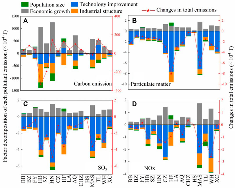
FIGURE 6. The contributions of factor decomposition to changes in industrial pollutant emissions, plotted against the changes in total emissions as of 2020. (Note: 2015 is the base year. Data on industrial NOx are missing for 2015.). (A) Carbon emission. (B) Particulate matter. (C) NO_x. (D) SO₂.

The evolution of NO₂ hotspots showed a gradual agglomeration to central Anhui. As NO₂ is one of the main precursors of O₃ formation, this indicates a high potential for O₃ formation in this region. Most of the O₃ break points occurred slightly after those of NO₂, and the hotspot evolution of O₃ was similar to that of NO₂. However, it should also be noted that O₃ formation is complex and includes various factors, such as the species, the contributions of various precursors (Li et al., 2022), inter-city transport, and meteorological conditions (Sulaymon et al., 2021). One study on the influence of atmospheric oxidation capacity on the dependence of PM_2.5–O₃ relationships in the YRD showed that, when the atmospheric oxidation capacity was relatively high, the correlation between PM_2.5 and O₃ was strong, and vice versa (Qin et al., 2022). A diagnosis of O₃ pollution in the summer of 2020 in Nanjing (Li et al., 2022) found that NOx and volatile organic compounds (VOCs) contributed to O₃ concentration (accounting for about 70% and 30%, respectively). Inter-city transport and intra-city emissions (from transportation and industry) accounted for 46% and 38% respectively, of the fluctuations in daily O₃ concentration, with alternating contributions from physical (vertical mixing and wind direction) and chemical (photochemical reactions) factors. Given that CZ, MAS, and WH are adjacent to Nanjing, and given the close connections between their respective economic development histories, the mutual migration of air pollutants among them was bound to occur. Figure 6C shows that the economic growth of these three cities (CZ, MAS, and WH) contributed the most to industrial NOx emissions.

By 2020, the CO hotspot was concentrated in the Wanjiang City Belt. Figure 6 also shows that the change in total industrial carbon emissions in the Wanjiang City Belt (comprising CZ, HF, LA, AQ, CHZ, MAS, TL, WH, and XC) from 2015 to 2020 was positive (with the exception of MAS). Previous studies on VOCs in different functional areas of HF city (Wang et al., 2021) confirmed that industrial areas contributed the most to the VOC concentration. Notably, technological improvements have contributed significantly to reducing industrial carbon emissions ( in HF and TL (Figure 6).

As the first Demonstration Zone for undertaking industrial transfer in Anhui province, the Wanjiang City Belt has gradually developed into new mega-urban agglomerations within the YRD and is now known as a hub for industrial transfer. For example, in HF city, we can see that population size has an effect on the growth of industrial pollutant emissions (Figure 6). Clearly, economic growth has significantly contributed to emissions of carbon and industrial pollutants (Wang et al., 2022), even as technological improvements and industrial structures have significantly inhibited industrial pollutant emissions (Figure 6). Geng et al. (2021) employed the LMDI model to examine the relative influence of four factors (economic growth, economic structure, energy-climate policy, and end-of-pipe control policy) on pollutant emissions (NOx, SO₂, and PM_2.5) in China. They found that economic growth was the main driving force behind pollutant emissions, with the remaining three factors having different degrees of inhibitory effects. This is consistent with the results of the present study. In this study, industrial structure was found to be more effective in reducing industrial carbon emissions, and technological improvement was found to be more advantageous in reducing industrial particulate matter, NOx, and SO₂ (Figure 6).

The obstacle degree analysis showed that particulate matter (PM₁₀ and PM_2.5), SO₂, and NO₂ were the primary obstacle factors. The seasonal differences in primary obstacle factors were most evident in 2020, including the dominance of NO₂ in winter (observed in 10 cities), SO₂ in southern Anhui, and particulate matter in northern and central Anhui in spring. Other seasons were almost entirely dominated by particulate matter. Meanwhile, in the winter of 2020, all the corresponding air quality indexes pointed to PM_2.5, even though 10 cities had NO₂ as their primary obstacle factor. This suggested that AQI did not always match the primary obstacle factor; that is to say, AQI alone could only reflect the primary pollutant, which was not necessarily the same as the primary obstacle factor. Moreover, it should be noted that the homogeneity of the primary obstacle factor on an annual scale may cover up any seasonal differences, and this discrepancy may pose difficulties for the accurate and effective formulation of air pollution prevention and control measures. The accurate diagnosis of obstacle degrees can therefore help optimize and quantify the primary obstacle factors among regional air pollutants, which is potentially of crucial practical significance for inter-regional joint prevention and control.

The mobility of air makes pollutants a highly externalized issue, and therefore the use of inter-regional collaborative governance to manage air pollution was an inevitable choice. The air quality of any city is affected by the dynamic superposition of air pollutants inside and outside the region (Gong et al., 2021). Simultaneously, air pollution has an obvious superposition effect because of the overall interaction relationship among the pollutants. Therefore, it is necessary to strengthen inter-regional joint prevention and control, undertake targeted measures specific to each city, co-manage, and avoid partial governance that applies only to individual cities.

First, the collaborative governance of air pollution prevention and control in the YRD should be seen as an impetus to strengthen the cooperative effects of inter-regional air pollution prevention and control. Although the collaborative governance of regional air pollution has obvious advantages in reducing the cost of emission reduction (Xiao Liu et al., 2022), the long-term effectiveness of the YRD’s regional air pollution policy is obviously insufficient (Wang and Zhao, 2021). Moreover, the collaborative governance of air pollutants (such as NOx-VOC) has benefits for human health and crop production (Ding et al., 2022). Therefore, it is necessary to strengthen the implementation of the integrated process of collaborative governance of air pollutants in the YRD; fully understand the importance of negotiation, shared responsibility, information sharing, and joint prevention and control; and form an inter-regional joint prevention and control mechanism with the same orientation but with a more specific focus.

Whether the coupling coordination degree was measured using intra-city air pollutants or inter-city AQI, we observed a sharp contrast between high coupling degree scores and low coordination degree scores. This result strongly supports the fact that a large degree of interaction between air pollutants, and obvious maladjustment, exists within and between cities. Second, the effects of the imbalances in economic growth level and industrial structure layout among the cities studied suggest that policies targeted to the specific causes of, and extent of, air pollution in different regions are likely the best method of managing these pollutants. For instance, in this study, technological improvement and industrial structure played a significant role in the decrease of industrial particulate matter emission; the inhibitory effect on industrial particulate matter emission in central and southern Anhui was better than that in northern Anhui (Figure 6B). Combined with the evolution of particulate matter hotspots (i.e., migration to northern Anhui), it was suggested that the technological improvement and industrial structure in northern Anhui should be continuously upgraded. Moreover, in the Wanjiang City Belt, where the CO hotspot eventually settled (matching the increase in total industrial carbon emissions), the industrial structure was more effective in reducing industrial carbon emissions (Figure 6A). Finally, the combined use of the primary obstacle factor and the AQI might help in the formulation of targeted measures to alleviate air pollution, thereby effectively reducing the cost of regional collaborative governance and clarifying the division of responsibilities.

Conclusion

The spatiotemporal dynamic evolution evaluation of air pollutants, combined with break point identification, coupling coordination degree model, obstacle degree model, and the ESDA, provides favorable technical support for implementation of regional joint prevention and control. Meanwhile, the LMDI model was applied to quantify the influence of economic growth, population size, technological improvement, and industrial structure on industrial pollutant emissions. The following conclusions were drawn:

(1) An objective approach to determining the break point might be helpful for timely feedback on the intensity of air pollution policy regulation. The O₃ levels in most cities reached their break point starting in 2018, but the break points of other air pollutants appeared earlier than that of O₃, mostly before 2018.

(2) The degree of interaction between air pollutants within each city of Anhui was relatively large, but these interactions did not reach a good level of coordinated development.

(3) Two main trends emerged from the evolution of air pollutant hotspots: agglomeration to central Anhui (NO₂ and O₃) and migration to northern Anhui (PM₁₀ and PM_2.5). CO eventually concentrated in the Wanjiang City Belt.

(4) The primary obstacle factors were particulate matter (PM₁₀ and PM_2.5), SO₂, and NO₂, with great seasonal differences. Meanwhile, industrial structure was more effective in reducing industrial carbon emissions, and technological improvement was more advantageous in reducing industrial particulate matter, NOx, and SO₂. The diagnosis of primary obstacle factors can be an effective complement to AQI in undertaking targeted measures for the alleviation of air pollution.

Data availability statement

The original contributions presented in the study are included in the article/Supplementary Material, further inquiries can be directed to the corresponding author.

Author contributions

HW: Conceptualization, software, data analysis, writing—review and editing. HG: Supervision, writing—review and editing. HW: Coordination, proofreading. GL: Supervision, methodology, writing—review and editing. All authors contributed to this article and approved the submitted version.

Funding

This research was funded by National Natural Science Foundation of China (41972166, 41773100) and Scientific Research Foundation for Outstanding Talents of Huaibei Normal University (03106128).

Conflict of interest

The authors declare that the research was conducted in the absence of any commercial or financial relationships that could be construed as a potential conflict of interest.

Publisher’s note

All claims expressed in this article are solely those of the authors and do not necessarily represent those of their affiliated organizations, or those of the publisher, the editors and the reviewers. Any product that may be evaluated in this article, or claim that may be made by its manufacturer, is not guaranteed or endorsed by the publisher.

Supplementary Material

The Supplementary Material for this article can be found online at: https://www.frontiersin.org/articles/10.3389/fenvs.2022.984879/full#supplementary-material

References

Ang, B. W. (2015). LMDI decomposition approach: A guide for implementation. Energy Policy 86, 233–238. doi:10.1016/j.enpol.2015.07.007

CrossRef Full Text | Google Scholar

Bai, X., Jin, J., Zhou, R., Wu, C., Zhou, Y., Zhang, L., et al. (2022). Coordination evaluation and obstacle factors recognition analysis of water resource spatial equilibrium system. Environ. Res. 210, 112913. doi:10.1016/j.envres.2022.112913

PubMed Abstract | CrossRef Full Text | Google Scholar

Chang, Y., Huang, Z., Ries, R. J., and Masanet, E. (2016). The embodied air pollutant emissions and water footprints of buildings in China: A quantification using disaggregated input–output life cycle inventory model. J. Clean. Prod. 113, 274–284. doi:10.1016/j.jclepro.2015.11.014

CrossRef Full Text | Google Scholar

Chen, Y., Xu, Y., and Wang, F. (2022). Air pollution effects of industrial transformation in the Yangtze River Delta from the perspective of spatial spillover. J. Geogr. Sci. 32 (1), 156–176. doi:10.1007/s11442-021-1929-6

CrossRef Full Text | Google Scholar

Cong, X. (2019). Expression and mathematical property of coupling model, and its misuse in geographical science. Econ. Geogr. 39 (4), 18–25. (in Chinese). doi:10.15957/j.cnki.jjdl.2019.04.003

CrossRef Full Text | Google Scholar

Deng, C., Tian, S., Li, Z., and Li, K. (2022). Spatiotemporal characteristics of PM2.5 and ozone concentrations in Chinese urban clusters. Chemosphere 295, 133813. doi:10.1016/j.chemosphere.2022.133813

PubMed Abstract | CrossRef Full Text | Google Scholar

Ding, D., Xing, J., Wang, S., Dong, Z., Zhang, F., Liu, S., et al. (2022). Optimization of a NO_x and VOC cooperative control strategy based on clean air benefits. Environ. Sci. Technol. 56 (2), 739–749. doi:10.1021/acs.est.1c04201

PubMed Abstract | CrossRef Full Text | Google Scholar

Dong, F., and Li, W. (2021). Research on the coupling coordination degree of “upstream-midstream-downstream” of China’s wind power industry chain. J. Clean. Prod. 283, 124633. doi:10.1016/j.jclepro.2020.124633

CrossRef Full Text | Google Scholar

Dong, Z., Xing, J., Zhang, F., Wang, S., Ding, D., Wang, H., et al. (2022). Synergetic PM2.5 and O3 control strategy for the Yangtze River delta, China. J. Environ. Sci. In Press. doi:10.1016/j.jes.2022.04.008

CrossRef Full Text | Google Scholar

Du, M., Liu, W., and Hao, Y. (2021). Spatial correlation of air pollution and its causes in northeast China. Int. J. Environ. Res. Public Health 18, 10619. doi:10.3390/ijerph182010619

PubMed Abstract | CrossRef Full Text | Google Scholar

Geng, G., Zheng, Y., Zhang, Q., Xue, T., Zhao, H., Tong, D., et al. (2021). Drivers of PM2.5 air pollution deaths in China 2002–2017. Nat. Geosci. 14 (9), 645–650. doi:10.1038/s41561-021-00792-3

CrossRef Full Text | Google Scholar

Gong, K., Li, L., Li, J., Qin, M., Wang, X., Ying, Q., et al. (2021). Quantifying the impacts of inter-city transport on air quality in the Yangtze River Delta urban agglomeration, China: Implications for regional cooperative controls of PM2.5 and O3. Sci. Total Environ. 779, 146619. doi:10.1016/j.scitotenv.2021.146619

PubMed Abstract | CrossRef Full Text | Google Scholar

Hao Li, H., Song, Y., and Zhang, M. (2017). Study on the gravity center evolution of air pollution in Yangtze River Delta of China. Nat. Hazards 90 (3), 1447–1459. doi:10.1007/s11069-017-3110-1

CrossRef Full Text | Google Scholar

Hites, R. A. (2019). Break point analyses of human or environmental temporal trends of POPs. Sci. Total Environ. 664, 518–521. doi:10.1016/j.scitotenv.2019.01.353

PubMed Abstract | CrossRef Full Text | Google Scholar

IPCC (2006). IPCC Guidelines for National Greenhouse Gas Inventories:volume II [EB/OL]. Japan: The Institute for Global Environmental Strategies. Available at: https://www.ipcc.ch/ipccreports/Methodology-reports.htm

Google Scholar

Jing Liu, J., Li, H., and Liu, T. (2022). Decoupling regional economic growth from industrial CO2 emissions: Empirical evidence from the 13 prefecture-level cities in jiangsu province. Sustainability 14, 2733. doi:10.3390/su14052733

CrossRef Full Text | Google Scholar

Li, K., Jacob, D. J., Liao, H., Shen, L., Zhang, Q., and Bates, K. H. (2019). Anthropogenic drivers of 2013-2017 trends in summer surface ozone in China. Proc. Natl. Acad. Sci. U. S. A. 116 (2), 422–427. doi:10.1073/pnas.1812168116

PubMed Abstract | CrossRef Full Text | Google Scholar

Li, L., Xie, F., Li, J., Gong, K., Xie, X., Qin, Y., et al. (2022). Diagnostic analysis of regional ozone pollution in Yangtze River delta, China: A case study in summer 2020. Sci. Total Environ. 812, 151511. doi:10.1016/j.scitotenv.2021.151511

PubMed Abstract | CrossRef Full Text | Google Scholar

Lin, B., and Long, H. (2016). Emissions reduction in China׳s chemical industry – based on LMDI. Renew. Sustain. Energy Rev. 53, 1348–1355. doi:10.1016/j.rser.2015.09.045

CrossRef Full Text | Google Scholar

Liu, W., Jiao, F., Ren, L., Xu, X., Wang, J., and Wang, X. (2018). Coupling coordination relationship between urbanization and atmospheric environment security in Jinan City. J. Clean. Prod. 204, 1–11. doi:10.1016/j.jclepro.2018.08.244

CrossRef Full Text | Google Scholar

Mi, K., Zhuang, R., Zhang, Z., Gao, J., and Pei, Q. (2019). Spatiotemporal characteristics of PM2.5 and its associated gas pollutants, a case in China. Sustain. Cities Soc. 45, 287–295. doi:10.1016/j.scs.2018.11.004

CrossRef Full Text | Google Scholar

Ministry of Ecology and Environment the People’s Republic of China (2021). Report on the state of the Ecology and environment in China 2020. Available at: https://english.mee.gov.cn/Resources/Reports/soe/ April 7, 2021).

Google Scholar

National Bureau of Statistics of China (2021). China statistical Yearbook. Available at: http://www.stats.gov.cn/tjsj/ndsj/2021/indexch.htm January 12, 2022).

Google Scholar

Pei, Z., Chen, X., Li, X., Liang, J., Lin, A., Li, S., et al. (2022). Impact of macroeconomic factors on ozone precursor emissions in China. J. Clean. Prod. 344, 130974. doi:10.1016/j.jclepro.2022.130974

CrossRef Full Text | Google Scholar

Qin, M., Hu, A., Mao, J., Li, X., Sheng, L., Sun, J., et al. (2022). PM2.5 and O3 relationships affected by the atmospheric oxidizing capacity in the Yangtze River Delta, China. Sci. Total Environ. 810, 152268. doi:10.1016/j.scitotenv.2021.152268

PubMed Abstract | CrossRef Full Text | Google Scholar

Salamova, A., Peverly, A. A., Venier, M., and Hites, R. A. (2016). Spatial and temporal trends of particle phase organophosphate ester concentrations in the Atmosphere of the great Lakes. Environ. Sci. Technol. 50 (24), 13249–13255. doi:10.1021/acs.est.6b04789

PubMed Abstract | CrossRef Full Text | Google Scholar

Su, Z., Lin, L., Chen, Y., and Hu, H. (2022). Understanding the distribution and drivers of PM2.5 concentrations in the Yangtze River delta from 2015 to 2020 using random forest regression. Environ. Monit. Assess. 194 (4), 284. doi:10.1007/s10661-022-09934-5

PubMed Abstract | CrossRef Full Text | Google Scholar

Sulaymon, I. D., Zhang, Y., Hopke, P. K., Hu, J., Rupakheti, D., Xie, X., et al. (2021). Influence of transboundary air pollution and meteorology on air quality in three major cities of Anhui Province, China. J. Clean. Prod. 329, 129641. doi:10.1016/j.jclepro.2021.129641

CrossRef Full Text | Google Scholar

Sun, Y., Wang, Y., and Zhang, Z. (2022). Economic environmental imbalance in China - inter-city air pollutant emission linkage in Beijing-Tianjin-Hebei (BTH) urban agglomeration. J. Environ. Manage. 308, 114601. doi:10.1016/j.jenvman.2022.114601

PubMed Abstract | CrossRef Full Text | Google Scholar

Tomal, M. (2020). Analysing the coupling coordination degree of socio-economic-infrastructural development and its obstacles: The case study of polish rural municipalities. Appl. Econ. Lett. 28 (13), 1098–1103. doi:10.1080/13504851.2020.1798341

CrossRef Full Text | Google Scholar

Wang, Z., Li, J., Wang, Z., Yang, W., Tang, X., Ge, B., et al. (2013). Modeling study of regional severe hazes over mid-eastern China in January 2013 and its implications on pollution prevention and control. Sci. China Earth Sci. 57 (1), 3–13. doi:10.1007/s11430-013-4793-0

CrossRef Full Text | Google Scholar

Wang, F., Wang, G., Liu, J., and Chen, H. (2019). How does urbanization affect carbon emission intensity under a hierarchical nesting structure? Empirical research on the China Yangtze River delta urban agglomeration. Environ. Sci. Pollut. Res. 26 (31), 31770–31785. doi:10.1007/s11356-019-06361-x

PubMed Abstract | CrossRef Full Text | Google Scholar

Wang, S., Liu, G., Zhang, H., Yi, M., Liu, Y., Hong, X., et al. (2021). Insight into the environmental monitoring and source apportionment of volatile organic compounds (VOCs) in various functional areas. Air Qual. Atmos. Health 15, 1121–1131. doi:10.1007/s11869-021-01090-y

CrossRef Full Text | Google Scholar

Wang, X., Iqbal, K., and Wang, Y. (2022). Energy use greenization, carbon dioxide emissions, and economic growth: An empirical analysis based in China. Front. Environ. Sci. 10, 871001. doi:10.3389/fenvs.2022.871001

CrossRef Full Text | Google Scholar

Wang, Y., and Zhao, Y. (2021). Is collaborative governance effective for air pollution prevention? A case study on the Yangtze River delta region of China. J. Environ. Manage. 292, 112709. doi:10.1016/j.jenvman.2021.112709

PubMed Abstract | CrossRef Full Text | Google Scholar

Wu, H., Guo, S., Guo, P., Shan, B., and Zhang, Y. (2022). Agricultural water and land resources allocation considering carbon sink/source and water scarcity/degradation footprint. Sci. Total Environ. 819, 152058. doi:10.1016/j.scitotenv.2021.152058

PubMed Abstract | CrossRef Full Text | Google Scholar

Xiang Li, X., Peng, L., Yao, X., Cui, S., Hu, Y., You, C., et al. (2017). Long short-term memory neural network for air pollutant concentration predictions: Method development and evaluation. Environ. Pollut. 231, 997–1004. doi:10.1016/j.envpol.2017.08.114

PubMed Abstract | CrossRef Full Text | Google Scholar

Xiao Liu, X., Wang, W., Wu, W., Zhang, L., and Wang, L. (2022). Using cooperative game model of air pollution governance to study the cost sharing in Yangtze River Delta region. J. Environ. Manage. 301, 113896. doi:10.1016/j.jenvman.2021.113896

PubMed Abstract | CrossRef Full Text | Google Scholar

Xiao, R., Lin, M., Fei, X., Li, Y., Zhang, Z., and Meng, Q. (2020). Exploring the interactive coercing relationship between urbanization and ecosystem service value in the Shanghai–Hangzhou Bay Metropolitan Region. J. Clean. Prod. 253, 119803. doi:10.1016/j.jclepro.2019.119803

CrossRef Full Text | Google Scholar

Xu, X., Zhang, Z., Long, T., Sun, S., and Gao, J. (2021). Mega-city region sustainability assessment and obstacles identification with GIS–entropy–TOPSIS model: A case in Yangtze River delta urban agglomeration, China. J. Clean. Prod. 294, 126147. doi:10.1016/j.jclepro.2021.126147

CrossRef Full Text | Google Scholar

Xu, P., Yang, Y., Zhang, J., Gao, W., Liu, Z., Hu, B., et al. (2022). Characterization and source identification of submicron aerosol during serious haze pollution periods in Beijing. J. Environ. Sci. 112, 25–37. doi:10.1016/j.jes.2021.04.005

PubMed Abstract | CrossRef Full Text | Google Scholar

Xue, H., Liu, G., Zhang, H., Hu, R., and Wang, X. (2019). Similarities and differences in PM10 and PM2.5 concentrations, chemical compositions and sources in Hefei City, China. Chemosphere 220, 760–765. doi:10.1016/j.chemosphere.2018.12.123

PubMed Abstract | CrossRef Full Text | Google Scholar

Yu, X., Wu, Z., Zheng, H., Li, M., and Tan, T. (2020). How urban agglomeration improve the emission efficiencyA spatial econometric analysis of the Yangtze River Delta urban agglomeration in China. J. Environ. Manage. 260, 110061. doi:10.1016/j.jenvman.2019.110061

PubMed Abstract | CrossRef Full Text | Google Scholar

Zhang, X., and Cheng, C. (2022). Temporal and spatial heterogeneity of PM2.5 related to meteorological and socioeconomic factors across China during 2000–2018. Int. J. Environ. Res. Public Health 19, 707. doi:10.3390/ijerph19020707

PubMed Abstract | CrossRef Full Text | Google Scholar

Zhao, H., Wang, L., Zhang, Z., Qi, Q., and Zhang, H. (2022). Quantifying ecological and health risks of ground-level O3 across China during the implementation of the "Three-year action plan for cleaner air. Sci. Total Environ. 817, 153011. doi:10.1016/j.scitotenv.2022.153011

PubMed Abstract | CrossRef Full Text | Google Scholar

Zheng, J., Zhang, L., Che, W., Zheng, Z., and Yin, S. (2009). A highly resolved temporal and spatial air pollutant emission inventory for the Pearl River Delta region, China and its uncertainty assessment. Atmos. Environ. X. 43 (32), 5112–5122. doi:10.1016/j.atmosenv.2009.04.060

CrossRef Full Text | Google Scholar

Zhou, J., Liu, G., Zhang, H., Liu, K., and Arif, M. (2021). Pollution characterization and source identification of nitrogen-containing species in fine particulates: A case study in Hefei city, east China. Chemosphere 285, 131316. doi:10.1016/j.chemosphere.2021.131316

PubMed Abstract | CrossRef Full Text | Google Scholar