Good environmental governance: Predicting PM2.5 by using Spatiotemporal Matrix Factorization generative adversarial network

In the context of low-carbon globalization, green development has become the common pursuit of all countries and the theme of China’s development in the new era. Fine particulate matter (PM2.5) is one of the main challenges affecting air quality, and how to accurately predict PM2.5 plays a pivotal role in environmental governance. However, traditional data-driven approaches and deep learning methods for prediction rarely consider spatiotemporal features. Furthermore, different regions always have various implicit or hidden states, which have rarely been considered in the off-the-shelf model. To solve these problems, this study proposed a novel Spatial-Temporal Matrix Factorization Generative Adversarial Network (ST MFGAN) to capture spatiotemporal correlations and overcome the regional diversity problem at the same time. Specifically, Generative Adversarial Network (GAN) composed of graph Convolutional Network (GCN) and Long-Short-Term Memory (LSTM) network is used to generate a large amount of reliable spatiotemporal data, and matrix factorization network is used to decompose the vector output by GAN into multiple sub-networks. PM2.5 are finally combined and jointly predicted by the fusion layer. Extensive experiments show the superiority of the newly designed method.

1 Introduction

With the rapid development of China’s economy and the acceleration of urbanization process, the excessive emission of pollutants has caused severe pollution to the air and impedes the process of sustainable development seriously (Chen and Li, 2021; Dong et al., 2021). In many industrial cities, coal is the regions’ lifeblood. Meanwhile, road transportation and automobile transportation have become the main ways of transporting goods, which leads to air pollution to a certain extent. PM2.5 is the primary air pollutant, which turns out to be the focus of China’s haze governance at this stage. PM2.5 harms human health, which has been brought to the center of public attention (Xing et al., 2021). If PM2.5 can be accurately predicted, which will have important implications for environmental management and human health. The concentration of PM2.5 is affected by urban spatial morphology, land use layout, and meteorological factors (Ma et al., 2019). Long-time exposure to air pollution will increase the risk of cardiovascular and respiratory disease (Ma et al., 2020). To find solutions, the Chinese government has set up air quality monitoring stations in most cities, which can monitor PM2.5 and other air pollutant concentration in real-time. Based on observed data, many researchers employ various models to predict PM2.5, which can provide guidance for government management (Gu et al., 2019). The PM2.5 prediction methods fall into two categories: model-driven and data-driven methods. The model-driven methods particularly estimate the PM2.5 concentration by establishing mathematical and statistical models. The data-driven methods predict PM2.5 concentration by using neural networks, support vector regression (SVR), and other machine learning models.

With the development of artificial intelligence and machine learning in recent years, methods such as artificial neural network (ANN) and SVR have been widely used in the prediction of air pollutant concentration. SVR model was employed to predict PM2.5 by using data from surrounding monitoring stations (Xiao et al., 2020). In Pak et al. (2020) research, A CNN-LSTM model was used to extract temporal and spatial features and predict PM2.5 of Beijing in China. However, there is currently rare work that consider the regional diversities. In different regions, the historical PM2.5 steady-state features of cities are usually different, and some cities follow the same pattern of the PM2.5 concentration (Du et al., 2021). There are three challenges in predicting PM2.5: spatial correlations, temporal correlations, and regional diversity. To cope with the challenges, this paper proposes a novel Spatial-Temporal Matrix Factorization Generative Adversarial Network called ST-MFGAN, which can capture spatiotemporal correlations and overcome regional diversity problems. Specifically, each component of GAN has a GCN-LSTM pipeline to capture spatiotemporal information. The output of the GAN is fed to dense layer and undergoes matrix decomposition to form multiple matrices. Each matrix is learned through an independent sub-net. These sub-net parameters will not interfere with each other and PM2.5 are finally combined and jointly predicted by the fusion layer. The main contributions of this paper are as follows:

1) In this paper, we propose a novel model, ST-MFGAN, to comprehensively consider spatiotemporal correlations and regional diversity. We design an ad-hoc predictor to achieve effectively prediction.

2) Most of PM2.5 prediction approaches do not adequately consider the spatiotemporal correlation within the datasets. In this paper, GAN is composed of GCN and LSTM, which can capture spatial information and temporal information to improve the performance of predicting PM2.5.

3) We verify our model and the other baselines in the PM2.5 prediction research line. Related results show that ST-MFGAN achieves a better performance compared with the existing models.

2 Related methods

2.1 GAN

GAN consists of two models: generator G and discriminator D, which are in a state of adversarial game. In the process of game (Goodfellow et al., 2014), generator plays the role of a liar, which can generate data similar to real data. The discriminator acts as a judge, distinguishing real data from generated data. G and D can be seen as players in two-player adversarial game. In theory, the discriminator and generator can achieve Nash equilibrium. In other words, the discriminator cannot distinguish between real data and generated data, the generator can generate data close to real data meanwhile. Based on this principle, the objective function V (G,D) of GAN is given as follows:

$V\left(G,D\right)=E_{x\sim P_{data}}\left[\log D\left(x\right)\right]+E_{z\sim P_z}[\log (1-D(G(z))](1)$

Where z represents random noise comes from the prior distribution, x samples from real data distribution, D(x) represents the probability that x come from the real data, and D [G(z)] is the probability that the input comes from the generated data rather than real data. In the training process of G, D [G(z)] tend to approach 1 as much as possible. In other words, G tries to minimize the objective function as much as possible. In the training process of D, D tries to maximize the objective function as much as possible. GANs have been gradually applied to prediction tasks recently due to admirable ability of feature extraction (Yoon et al., 2019), which has inspired a myriad of follow-ups to employ GAN to generation and prediction tasks. Considering that, employing GAN to PM2.5 prediction is appealing for this paper.

2.2 GNN

GNN has achieved state-of-the-art results on various graph-based learning tasks, such as a node or link classification. In recent studies, the mainstream of GNNs fall into Graph Convolutional Network (Kipf and Welling, 2016) and Graph attention network (Velickovic et al., 2017). Due to the powerful fitting abilities on non-Euclidean data, graph neural networks have been applied to fields such as social networks, knowledge graphs, molecular structures, and traffic networks. However, we focus on the variants of GNNs in the field of pollutant prediction in this paper.

2.3 LSTM

LSTM (Hochreiter and Schmidhuber, 1997) is a type of Recurrent Neural Network (RNN), which is designed to solve gradient explosion in RNN, and it is usually used for time series prediction. LSTM consists of three parts, namely the input gate, the output gate and the forget gate. The network structure of LSTM can be shown as Figure 1. LSTM is widely used to predict time series.

FIGURE 1

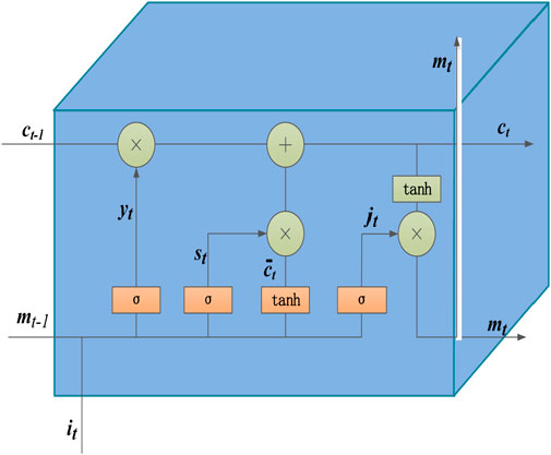
FIGURE 1. The architecture of LSTM.

3 Prediction model via adversarial training

3.1 The establishment of PM2.5 prediction model via adversarial training

This paper proposes a PM2.5 prediction model based on GAN, named ST-MFGAN. The framework of ST-MFGAN can be constructed as Figure 2. The random noise is fed to the generator, and generator output data with spatiotemporal information similar to the real data. The real PM2.5 and generated PM2.5 concentration are fed to a dense layer. Then, a matrix factorization layer filters various regional hidden information in different sub-network. Finally, we use the fusion layer to utilize all the different hidden state information for collaborative prediction. When constructing the loss function of the generator, the MSE loss is added to original objective function of GAN, which can reduce the instability of GAN during training. The loss functions of the generator and the discriminator can be described as:

$D_{loss}=-\frac{1}{n}{\displaystyle \sum }_{i=1}^n\log D\left(x\right)-\frac{1}{m}{\displaystyle \sum }_{i=1}^n\log D\left(1-D\left(G\left(z\right)\right)\right)(2)$

$g_{loss}=\frac{1}{n}{\displaystyle \sum }_{i=1}^n\log \left(1-D\left(G\left(z\right)\right)\right)(3)$

$G_{loss}=a{g}_{MSE}+b{g}_{loss}(4)$

FIGURE 2

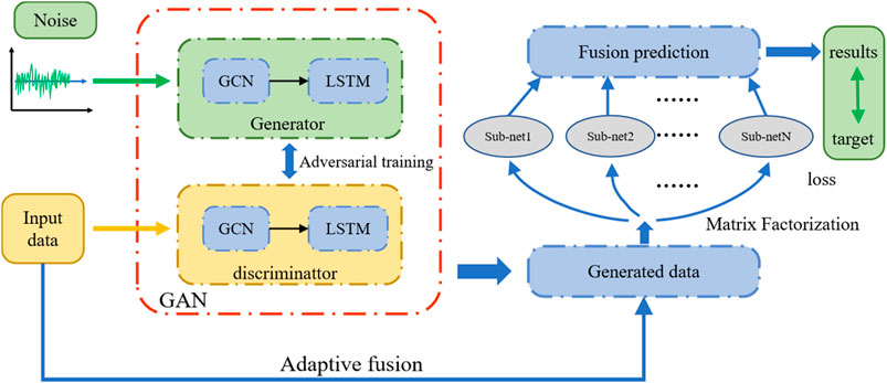
FIGURE 2. The framework of ST-MFGAN.

The loss function of the G consists of two parts, a and b are manually set hyperparameters, considering that the proportion of a and b should be the same, so a and b are both 0.5.

3.2 Modified GCN and LSTM for spatiotemporal information capturing

PM2.5 contains ammonium nitrate, which is easily decomposed when the temperature is high. Ammonium nitrate is also easily deliquescent, so temperature and humidity are closely correlated with PM2.5. The wind and vortex help the PM2.5 concentration in the air to spread horizontally and vertically, so the wind speed and vortex state are both related to PM2.5. Precipitation acts as a resistance to PM2.5 concentration, which will produce moisture removal and downward airflow. Therefore, precipitation can be also closely correlated with PM2.5 concentration. Based on the above analysis, this paper chooses time, temperature, humidity, wind speed, precipitation and other variables as input to predict the change of PM2.5 concentration. Assuming that the input matrix X = {x₁, x₂,…, x_t}, X represents data at t time points, where x₁, x₂,…, x_t represent time, temperature, humidity, wind speed, precipitation and vortex status at t time respectively. GCN and LSTM are added to the generator and discriminator of GAN due to strong feature extraction capabilities of them. This paper selects historical air data of different cities in the Beijing-Tianjin-Hebei region of China from the ERA5 datasets. Assuming that the input matrix $X_i=\left\{X_i^{\mathit{1}},X_i^{\mathit{2}}\dots X_i^M\right\}$, $X$ represents input data, where $X_i$ represent $i\_th$ city, M represents total time intervals. GCN and LSTM are added to the GAN generator and discriminator to capture spatial and temporal information, respectively. Similarly, $Y=\left\{Y_{\mathit{1}},Y_{\mathit{2}}\dots Y_N\right\}=\{\left\{Y_{\mathit{1}}^{\mathit{1}},Y_{\mathit{1}}^{\mathit{2}}\dots Y_{\mathit{1}}^M\right\},\left\{Y_{\mathit{2}}^{\mathit{1}},Y_{\mathit{2}}^{\mathit{2}}\dots Y\right\}\dots \{Y_N^{\mathit{1}},Y_N^{\mathit{2}}\dots Y_N^M\}$, where $Y$is label information. Here, to fully use spatial information, we modified traditional GCN aggregation matrix. Traditional GCN follows layer-wise propagation:

$H^{l+\mathit{1}}=\sigma \left(\stackrel{\sim }{A}\cdot H^l\cdot W\right)(5)$

Here $\stackrel{\sim }{A}$ is adjacency matrix of graph with added self-connections. $H^l$ and $H^{l+1}$ are outputs of (l-1)-th and l-th layers. $H^{\mathit{0}}=X$ is input data. In this paper, we modified $\stackrel{\sim }{A}$ , assuming that two city pattern similarity can be calculate as:

${\mathbb{M}}_t\left(x_i^t,x_j^t\right)=(\overrightarrow{x_i^t}\cdot \overrightarrow{x_j^t})/|\overrightarrow{x_i^t}|\cdot \left|\overrightarrow{x_j^t}\right|(6)$

Then, we can represent adjacency matrix as:

$A_t=\left(\begin{array}{ccc}{\mathbb{M}}_t\left(x_1^t,x_1^t\right)& \cdots & {\mathbb{M}}_t\left(x_1^t,x_N^t\right)\\ ⋮& \ddots & ⋮\\ {\mathbb{M}}_t\left(x_N^t,x_1^t\right)& \cdots & {\mathbb{M}}_t\left(x_N^t,x_N^t\right)\end{array}\right)(7)$

By this way, our modified GCN can be represent as:

$H^{l+\mathit{1}}\left(t\right)=\sigma \left(A_t\cdot H^l\left(t\right)\cdot W\left(t\right)\right)(8)$

And then the output of GCN is fed to LSTM. We perform spatiotemporal learning on the input data to GCN and LSTM and conduct adversarial training to generate data similar to real data.

3.3 Matrix factorization networks

Matrix factorization introduces a large number of parameters to learn the differences of different subregions. Each parameter subset learns independently and does not interfere with each other, which ensures the independence and reliability of the prediction of each region.Therefore, matrix factorization network is widely used in deep learning due to the advantage for spatio-temporal data in recent years (Wang and Ma, 2021). In order to predict PM2.5 more accurately, the real data $x$ and the generated data $G\left(z\right)$ in Section 3.2 are combined together in a certain proportion. Then we propose the formula: $X_c=x+\gamma G\left(z\right)$, where $X_c$ denotes the hyperparameter for adjusting the ratio of $x$ and $G\left(z\right)$. After generated data through generator of GAN, the corresponding vectors is generated through the dense layer. And we assume that the network structure of the vectors is $F^{\prime }\in R^{n_f\times n_{f^{\prime }}}$. Then, the matrix decomposition network can be used to make adaptive adjustments to the number of variable regions in the network, and the matrix decomposition network can be written as $W=\left[W_1,\dots W_{nr}\right]\in R^{n_r\times n_{f^{\prime }}\times n_f},W_i\in R^{n_f\times n_f}$.

We suppose $R=\left[r_1,\dots r_{nr}\right]\in R^{n_r\times R}$ and $P=\left[p_1,\cdots ,p_{np}\right]\in R^{n_p\times R}$, where $n_p=n_f\times n_{f^{\prime }}$. To make the process of matrix decomposition more smooth, we suppose $W=R{P}^T$, then the learning targets are revised as R and P. The output of the MF network can be expressed as $f_i^{\prime }={\omega }_i\cdot f_i+b_i,i=1\to n_r$. And $f_i^{\prime }\left(i=1\to n_r\right)$ is combined by the fully connected layer, which is used to jointly predict PM2.5.

3.4 Model summary

In this paper, ST-MFGAN is proposed to predict PM2.5. The generator and discriminator consist of GCN and LSTM, which can capture spatiotemporal correlations among the inputs and overcome the regional diversity problem. Matrix factorization networks is also used to make adaptive adjustments to the number of variable regions in this model, which can effectively reduce the interference between the parameters of each sub-network, and it can be used to predict PM2.5 more accurately compared to other models. In order to verify the effectiveness and superiority of the proposed method, comparative experiments and ablation experiments will be conducted in next section.

4 Experiment and result analysis

ERA5 dataset is used in this paper, and the historical air data of 13 cities in the Beijing-Tianjin-Hebei region are selected. It can make sense to choose this dataset since these cities are with more severe air pollution in China. Air data for the period 2015–2018 are selected from the data set of 13 cities in experiments. When dividing the data set, 3-year data from January 2015 to December 2017 is used for the training set, and data from January to December 2018 is selected for the testing set. To eliminate the dimensional influences between different indicators, we normalize all the features in the datasets, which is shown as:

$x_i=\frac{{\mathit{X}}_i-\mathit{\mu }}{\mathit{\tau }}(9)$

Where $\mu$ and $\tau$ represent the mean value and variance of X. In the training process of ST-MFGAN, in order to prevent the discriminator or generator from being locally optimal, the discriminator and generator alternately iterate. After each iteration of the discriminator, the generator then iterates once. The training of ST-MFGAN will continue until the model is stable. All experiments in this paper are conducted based on Nvidia 3,090 (24 GB) and Tensorflow, which is an open source machine learning framework. In the experiment, the epochs are set to 200, the batch-size is 64, the number of neurons in each layer of LSTM is 8, and the dropout value is 0.1, the learning rate is set at 0.01, and Adam optimizer is used to updates the network. In order to find the optimal number of LSTM and GCN blocks, this paper conducts experiments by setting different blocks. The results of the experiments are shown in Figure 3. It can be seen that the RMSE is the smallest when the number of LSTM blocks is set to two and the number of GCN blocks is 1. Therefore, the number of LSTM modules is set to two and the number of GCN modules is set to one in this paper. Figure 4 shows the weights of the two LSTM blocks, from which it can be seen that the weights are updated when the input data are passed through each of the two LSTM blocks.

FIGURE 3

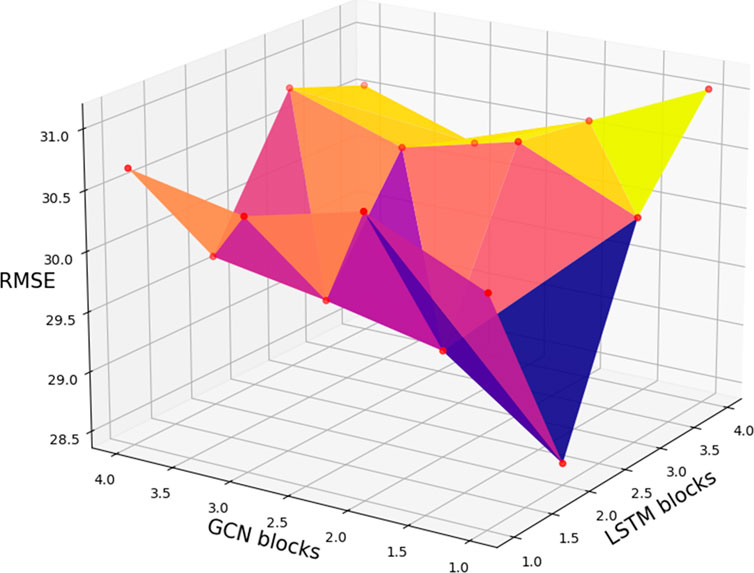
FIGURE 3. The RMSE based on different GCN and LSTM blocks.

FIGURE 4

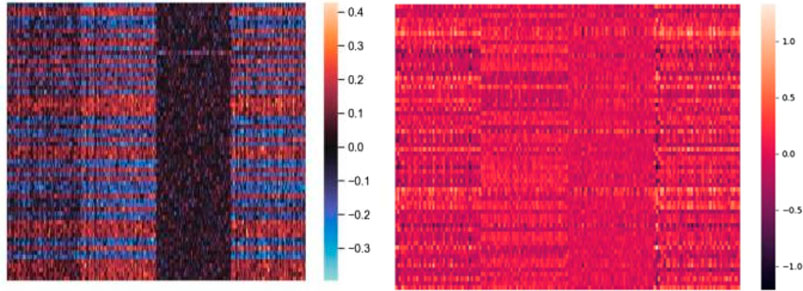
FIGURE 4. The weights change between LSTM blocks.

To verify the effectiveness and superiority of the proposed method, comparative experiments with other mainstream data-driven methods are conducted. We adopot six different models of GRU, LSTM, CNN-GRU, CNN-LSTM, IDW-LSTM, RBF-LSTM as baseline for this paper. GRU, LSTM, CNN-GRU, CNN-LSTM are the basic regression prediction models, which are widely used in PM2.5 prediction. IDW-LSTM is a methodology framework for PM2.5 prediction, which consists of inverse distance weighting and BLSTM (Ma et al., 2019). RBF-LSTM is proposed to forecast PM2.5 concentration, which consists of radial basis function and LSTM (Chen and Li, 2021). In the comparative experiments in this paper, the number of GRU layers of the GRU method is set to 2. In CNN-GRU, the number of CNN layers is set to 1, and the number of GRU layers is 2. The number of CNN layers in CNN-LSTM is 1, and the number of LSTM layers is 2. In IDW-LSTM, the number of BLSTM layers is 2. In LSTM and RBF-LSTM, the number of LSTM layers is 2. The training loss curves of seven models are shown in Figure 5. It can be seen from Figure 5, the loss of seven models do not decrease at the later stage of traing process, which indicates that all models are fully trained, which reflects the rigor and fairness of this paper to a certain extent. As can be seen from Figure 5, the loss of ST-MFGAN decreases fast during the training process and fluctuates less significantly in the later stages of training, which verifies that proposed model is stable during training. This can further indicate that proposed model can be better applied to predict PM2.5.

FIGURE 5

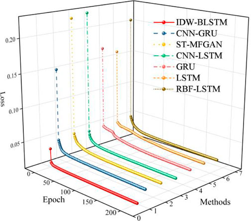
FIGURE 5. The training loss of different models.

The PM2.5 prediction results on the Baoding test set are shown in Figure 6. As can be seen from Figure 6, the prediction curve of ST-MFGAN is closer to that of the actual PM2.5 compared with other models. Especially, when the real PM2.5 turn to be a brief peak, ST-MFGAN is more able to estimate the trend of PM2.5 and can predict more accurately than other models. As shown in Figures 7–13, the prediction effect of each method can be presented more clearly. The performance of ST-MFGAN is significantly better than other comparative models. In terms of the prediction performance, ST-MFGAN can predict the trend of PM2.5 more accurately.

FIGURE 6

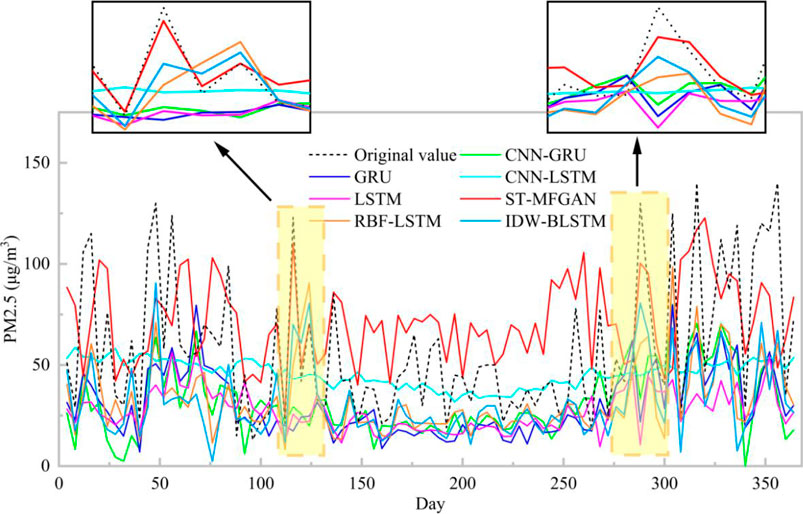
FIGURE 6. Experimental results of different methods on the Baoding test set.

FIGURE 7

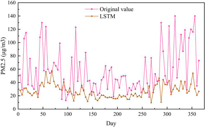
FIGURE 7. Experimental results of LSTM method in Baoding test set.

FIGURE 8

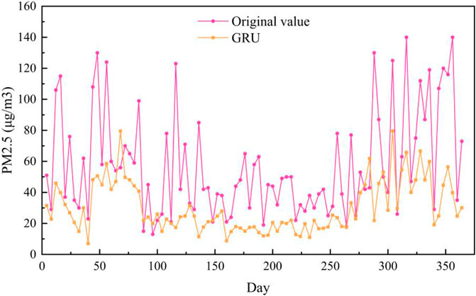
FIGURE 8. Experimental results of GRU method in Baoding test set.

FIGURE 9

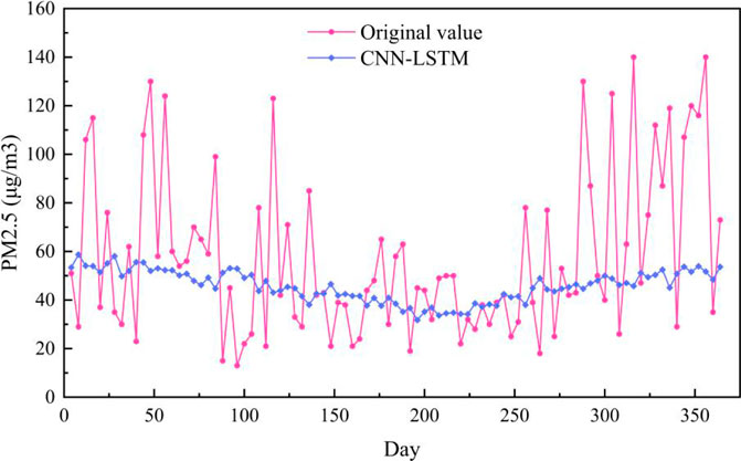
FIGURE 9. Experimental results of CNN-LSTM method in Baoding test set.

FIGURE 10

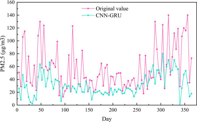
FIGURE 10. Experimental results of CNN-GRU method in Baoding test set.

FIGURE 11

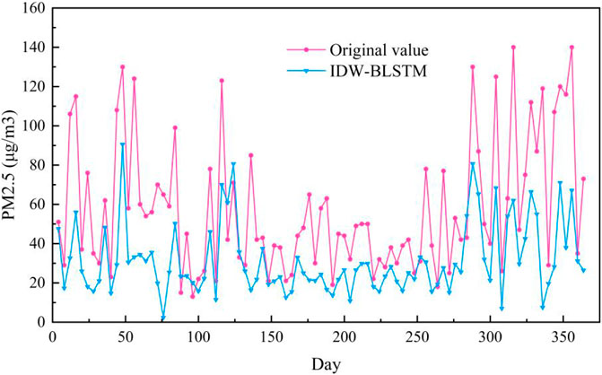
FIGURE 11. Experimental results of IDW-LSTM method in Baoding test set.

FIGURE 12

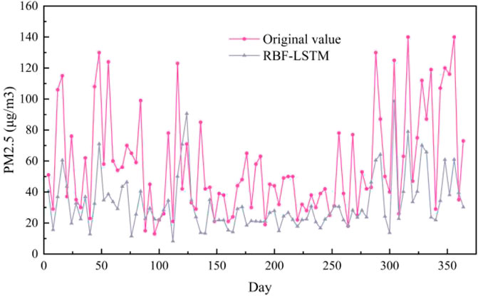
FIGURE 12. Experimental results of RBF-LSTM method in Baoding test set.

FIGURE 13

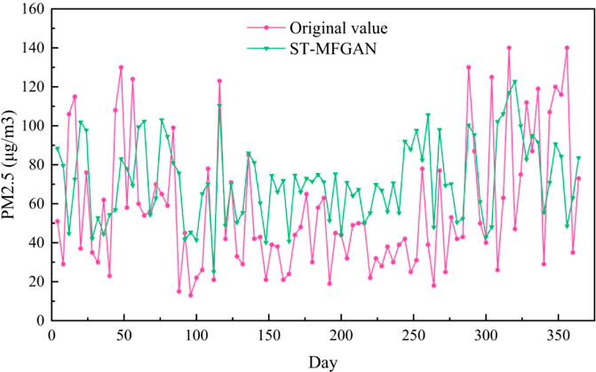
FIGURE 13. Experimental results of ST-MFGAN method in Baoding test set.

In order to more intuitively describe the prediction accuracy of various methods, the root mean square error (RMSE) and mean absolute error (MAE) are adopted to evaluate the prediction performance of each model. The calculation of RMSE and MAE is defined as:

$RMSE=\sqrt{\frac{1}{m}{\displaystyle \sum }_{k=1}^m{\left(\stackrel{\wedge }{y_k}-y_k\right)}^2}(10)$

$MAE=\frac{1}{m}{\displaystyle \sum }_{k=1}^m\left|\stackrel{\wedge }{y_k}-y_k\right|(11)$

Where $\stackrel{\wedge }{y_k}$ represents the predicted PM2.5 concentration, and $y_k$ is the actual PM2.5 concentration. The smaller the value of MAE and RMSE are, the closer the predicted PM2.5 are to the actual PM2.5. In order to ensure the reliability of the experiments, repeated experiments are carried out in this paper, and the average value of multiple experiments is taken as the result of MAE and RMSE. From the results in Table 1, it can be concluded that the RMSE and MAE of ST-MFGAN are the smallest among the seven models. The predicted PM2.5 concentration of ST-MFGAN is closer to the actual PM2.5 concentration, and the performance of the prediction is better than the others. It fully verifies the effectiveness of the proposed ST-MFGAN model. From Figure 14 and Figure 15, it can be seen more intuitively that ST-MFGAN has the lowest MAE and RMSE, which denotes that ST-MFGAN achieves the best performance of PM2.5 prediction.

TABLE 1

TABLE 1. The RMSE and MAE of the five methods in the test set.

FIGURE 14

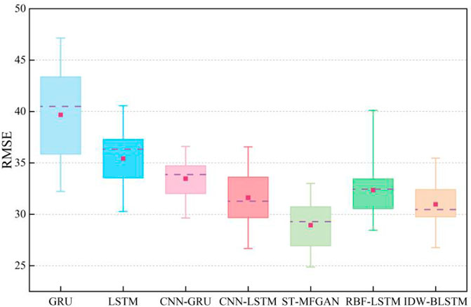
FIGURE 14. RMSE of different methods on the test set.

FIGURE 15

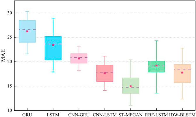
FIGURE 15. MAE of different methods on the test set.

To further verify the validity of the model structure proposed in this paper, ablation experiments were conducted in this paper. We compare ST-MFGAN with the original GAN, GCN-GAN (GAN with generator of GCN), and LSTM-GAN (GAN with generator of LSTM), and experiments results are shown in Table 2.

TABLE 2

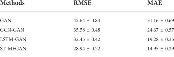
TABLE 2. The RMSE and MAE of the ablation experiments in the test set.

It can be seen from the ablation experimental results that ST-MFGAN achieves the best prediction performance due to hitting lower RMSE and MAE, which further verifies the effectiveness of the model structure proposed in this paper.

5 Conclusion

This paper propose a PM2.5 prediction method based on ST-MFGAN. The generator and discriminator consist of GCN and LSTM, which can capture spatiotemporal correlations among the inputs compared with original GAN, and it can overcome the regional diversity problem. Matrix factorization networks are also used to make adaptive adjustments to the number of variable regions in this model. Compared with PM2.5 prediction methods based on LSTM, GRU, CNN-LSTM and CNN-GRU, IDW-LSTM, and RBF-LSTM, the method in this paper has a better prediction performance, which can be used in governing environment. It can be seen from the results of this paper that PM2.5 concentration changes periodically and is difficult to control. Therefore, the government needs to strengthen environmental management and introduces a series of powerful policies to control the concentration of PM2.5.

Although the PM2.5 prediction method of ST-MFGAN can effectively predict the concentration of PM2.5, there is still room for further improvement of this paper. Most studies on PM2.5 prediction use various meteorological variables to predict PM2.5. However, few studies currently take policy factors into account. Future research can take the policy into consideration, which may improve the forecasting effect of PM2.5. Compared with GRU, LSTM and other models, GAN may bring additional cost during the training process. Future research can focus on the study of lightweight GAN for PM2.5 prediction, which can reduce the number of parameters of the model so that GAN can be trained and predicted more quickly in the prediction task.

Data availability statement

The original contributions presented in the study are included in the article/Supplementary Material, further inquiries can be directed to the corresponding author.

Author contributions

All authors contributed to this research. AZ completed the experiment of this paper and completed the writing of this article. SC provided ideological guidance for this research. FZ was an reviewer in editing this paper. XD also provided ideological guidance for this research. All authors approved this final manuscipt.

Funding

This work supported by Research Program supported by Fundamental Research Funds from the Central Universities (CN) (Nos. 2021CDJSKPT05, 2020CDJSK01WT07) and the National Natural Science Foundation of China (No. 72274026).

Conflict of interest

The authors declare that the research was conducted in the absence of any commercial or financial relationships that could be construed as a potential conflict of interest.

Publisher’s note

All claims expressed in this article are solely those of the authors and do not necessarily represent those of their affiliated organizations, or those of the publisher, the editors and the reviewers. Any product that may be evaluated in this article, or claim that may be made by its manufacturer, is not guaranteed or endorsed by the publisher.

References

Chen, Y. C., and Li, D. C. (2021). Selection of key features for PM2.5 prediction using a wavelet model and RBF-LSTM. Appl. Intell. (Dordr). 51, 2534–2555. doi:10.1007/s10489-020-02031-5

CrossRef Full Text | Google Scholar

Dong, Z., Li, L., Lei, Y., Wu, S., Yan, D., and Chen, H. (2021). The economic loss of public health from PM2.5 pollution in the Fenwei Plain. Environ. Sci. Pollut. Res. 28, 2415–2425. doi:10.1007/s11356-020-10651-0

CrossRef Full Text | Google Scholar

Du, P., Wang, J., Yang, W., and Niu, T. (2021). A novel hybrid fine particulate matter (pm2.5) forecasting and its further application system: Case studies in China. J. Forecast. 41, 64–85. doi:10.1002/for.2785

CrossRef Full Text | Google Scholar

Goodfellow, I. J., Pouget-Abadie, J., Mirza, M., Xu, B., Warde-Farley, D., Ozair, S., et al. (2014). Generative adversarial networks. Commun. ACM 3, 139–144. doi:10.1145/3422622

CrossRef Full Text | Google Scholar

Gu, K., Qiao, J., and Li, X. (2019). Highly efficient picture-based prediction of PM2.5 concentration. IEEE Trans. Ind. Electron. 66, 3176–3184. doi:10.1109/TIE.2018.2840515

CrossRef Full Text | Google Scholar

Hochreiter, S., and Schmidhuber, J. (1997). Long short-term memory. Neural Comput. 9 (8), 1735–1780. doi:10.1162/neco.1997.9.8.1735

PubMed Abstract | CrossRef Full Text | Google Scholar

Kipf, T. N., and Welling, M. (2016). Semi-supervised classification with graph convolutional networks. arXiv.

Google Scholar

Ma, J., Ding, Y., Gan, V., Lin, C., and Wan, Z. (2019). Spatiotemporal prediction of PM2.5 concentrations at different time granularities using IDW-BLSTM. IEEE Access 7, 107897–107907. doi:10.1109/ACCESS.2019.2932445

CrossRef Full Text | Google Scholar

Ma, J., Ding, Y., Jack, C., Cheng, P., Jiang, F., Gan, V. J. L., et al. (2020). A Lag-FLSTM deep learning network based on Bayesian Optimization for multi-sequential-variant PM2.5 prediction. Sustain. Cities Soc. 60, 102237. doi:10.1016/j.scs.2020.102237

CrossRef Full Text | Google Scholar

Pak, U., Ma, J., Ryu, U., Ryom, K., Juhyok, U., Pak, K., et al. (2020). Deep learning-based PM2. 5 prediction considering the spatiotemporal correlations: A case study of beijing, China. Sci. Total Environ. 699, 133561. doi:10.1016/j.scitotenv.2019.07.367

PubMed Abstract | CrossRef Full Text | Google Scholar

Velickovic, P., Cucurull, G., Casanova, A., Romero, A., Lio, P., and Bengio, Y. (2017). Graph attention networks. arXiv.

Google Scholar

Wang, Y., and Ma, X. K. (2021). Joint nonnegative matrix factorization and network embedding for graph co-clustering. Neurocomputing 462, 453–465. doi:10.1016/j.neucom.2021.08.014

CrossRef Full Text | Google Scholar

Xiao, Y., Zhao, J., Liu, H., Wang, L., and Liu, J. (2020). Dynamic prediction of pm2.5 diffusion in urban residential areas in severely cold regions based on an improved urban canopy model. Sustain. Cities Soc. 62, 102352. doi:10.1016/j.scs.2020.102352

CrossRef Full Text | Google Scholar

Xing, H., Wang, G., Liu, C., and Suo, M. (2021). Pm2.5 concentration modeling and prediction by using temperature-based deep belief network. Neural Netw. 133, 157–165. doi:10.1016/j.neunet.2020.10.013

PubMed Abstract | CrossRef Full Text | Google Scholar

Yoon, J., Jarrett, D., and Schaar, M. (2019). Time-series generative adversarial networks. Adv. neural Inf. Process. Syst. 32.

Google Scholar