Spatiotemporal characteristics and influencing factors of agricultural low-carbon economic efficiency in china

Developing low-carbon agriculture can effectively avoid the waste of natural resources, thus contributing to the long-term sustainability of agriculture. This study uses the Super-SBM model to measure agricultural low-carbon economic efficiency (ALEE) in China from 2000 to 2018, then analyzes the spatial-temporal evolution characteristics. Simultaneously, the influencing factors of ALEE are investigated using spatial econometric model. The results show that: (1) In terms of temporal evolution, the ALEE in most provinces is declined over time, with only a few provinces improving. The ALEE in China and the three regions all show an obvious “L” trend of decline first and then stability. (2) From the perspective of spatial differentiation, provinces in eastern region have higher ALEE, while those in central and western regions have lower ALEE. Hainan’s ALEE has an absolute advantage, while Shanxi is the worst. (3) China’s ALEE shows obvious spatial agglomeration characteristics of H-H and L-L agglomeration, which are further enhanced over time. The number of L-L agglomeration provinces gradually increases, indicating that China’s ALEE has not been improved significantly. (4) Economic growth level and Agricultural scientific and Technological progress have effectively improved the ALEE. However, Capital deepening, Government fiscal expenditure, Agricultural planting structure, and Agricultural disaster all have negative impacts. Rural electricity consumption also has a negative impact, but the impact is not significant. To accelerate the development of low-carbon agriculture, all regions must not only pursue a differentiated low-carbon agriculture development path, but also accelerate agricultural transformation, strengthen research and development, and popularize low-carbon agricultural technologies, reduce the input of traditional agricultural means of production, optimize the agricultural industrial structure, and adjust agricultural subsidy policies.

1 Introduction

All nations are paying more attention to low-carbon development due to the rising greenhouse gas emissions, and many countermeasures are being taken. China, as the country with the highest total carbon emissions (Yang et al., 2019), made it clear that it will strive to reach the peak of carbon dioxide emissions by 2030 and carbon neutrality by 2060 at the 75th United Nations General Assembly in 2020. This goal establishes a higher standard for China’s low-carbon development. However, for a long time, the main battlefield of energy conservation and carbon emission reduction have been in industry, energy, transportation, and other similar fields. Agriculture has not received enough attention (Xiong et al., 2021). China relies heavily on the high-carbon agricultural production mode, which means achieving major progress in agriculture at the cost of large energy consumption and serious environmental pollution. (Yang et al., 2018). However, high-carbon agricultural production mode depends heavily on the agricultural materials such as chemical fertilizers, pesticides, and agricultural films. (Rural Social Economic Investigation Division and National Bureau of Statistics of China, 2018). Overuse of these agricultural materials causes a large area of agricultural non-point source pollution and an ongoing increase of China’s agricultural carbon emissions. (Ren et al., 2021). From the available data, agricultural carbon emissions account for 11% of the total global carbon emissions. In China, it is 17%. And the overall trend is increasing year by year, posing a serious environmental threat (Huang et al., 2019). There is much room for energy conservation and carbon emission reduction in agriculture (Yang et al., 2022). However, how to promote the development of low-carbon agriculture while maintaining the stable and sustainable growth of agricultural economy is a pressing issue that must be addressed. Undoubtedly, studying the spatiotemporal evolution characteristics and influencing factors of China’s ALEE and is critical.

Based on this, this paper makes breakthroughs in two aspects. The first is to adopt the ALEE index. The low-carbon economy is defined as “activities that generate products or services with low carbon outputs.” (DBIS, 2015) ALEE refers to obtaining as much expected output (gross agricultural output value) and as little unexpected output (carbon emissions) as possible while maintaining inputs such as agricultural labor, land, irrigation, chemical materials and agricultural power. The essence of ALEE is agricultural productivity under low-carbon constraints, which refers to the agricultural low-carbon development level based on agricultural factor inputs. In fact, we constructs a more comprehensive agricultural total factor productivity measurement indicator system to obtain more scientific and accurate results. Second, this paper measures China’s ALEE and analyzes its temporal and spatial characteristics using the Super-SBM model. The spatial panel data model with spatial effect is established based on the principle of spatial economics, and the influencing factors of ALEE can be accurately identified by improving the accuracy of the model estimation results.

2 Literature review

For a long time, high-carbon agriculture has caused significant environmental damage, so it is critical to research an environmentally friendly, ecological, and efficient low-carbon agriculture model. Therefore, academia is increasingly interested in low-carbon agriculture. There are two ways to reduce the accumulation of greenhouse gases in the atmosphere: reducing carbon emissions sources and increasing carbon sinks (Li, 2014). Therefore, the literature on low-carbon agriculture mainly focuses on agricultural productivity and agricultural carbon sinks.

Some research on low-carbon agriculture was primarily reflected in the specific input uses of the agricultural sector, such as water use efficiency (Geng et al., 2019; Cao et al., 2020) and fertilizer use efficiency (Huang and Jiang, 2019; He et al., 2020). Scholars found that these indexes are too single to reflect the level of agricultural comprehensive development. Therefore, they gradually studied agricultural total factor productivity. However, the traditional method of calculating agricultural total factor productivity only considers economic output (Toma et al., 2017; Diao et al., 2018; Skevas et al., 2018), ignoring the negative impact of pollution. The environmental constraint is not considered in this productivity calculation, hence there will always be a divergence. To address this issue, many researchers incorporated unexpected output into the agricultural productivity evaluation system and considered agricultural productivity under environmental constraints (Liu and Feng, 2019; Hamid and Wang, 2022). In addition to measuring agricultural production efficiency, scholars also explored its spatial differentiation and influencing factors (Xiong et al., 2021; Chopra et al., 2022). It is crucial to analyze the spatial characteristics of agricultural production efficiency for rational utilization of natural resources (Hu et al., 2022). And studying the influencing factors of agricultural production efficiency is the basis for the country to accurately formulate agricultural reform policies (Zhou et al., 2021).

Scholars usually use stochastic frontier analysis (SFA) and data envelopment analysis (DEA) to calculate agricultural total factor productivity (Benedetti et al., 2019; Shen et al., 2019; Adetutu and Ajayi, 2020). SFA model requires the establishment of specific production functions, which is limited in practice (Xu et al., 2020). DEA, which is applicable to multi-input and multi-output boundary production functions (Bai et al., 2019), can solve this problem. DEA has therefore become primary method of calculating agricultural productivity (Emrouznejad and Yang, 2018). Chen et al. (2021) employed the three-stage DEA method to investigate agricultural total factor productivity. Huang et al. (2022)measured and tested the robustness of China’s agricultural total factor productivity using two different DEA models.

However, the efficiency value calculated by the above DEA model cannot be greater than one, implying that the differences between decision-making units are not accurately reflected. Therefore, some scholars gradually began to use the Super-SBM model to calculate agricultural total factor productivity, which breaks through the limitation of efficiency value 1 and improved accuracy. Liu et al. (2020); Chi et al. (2022) used the Super-SBM model to calculate agricultural ecological efficiency. Liu et al. (2021) calculated agricultural total factor productivity based on the Super-SBM model. However, there is still a lack of research on ALEE based on the Super-SBM model.

Apart from studying low-carbon agriculture from the perspective of productivity, scholars have gradually realized the importance of carbon sink research for the development of low-carbon agriculture. The research on agricultural carbon sink is mainly concentrated in foreign countries (Kim et al., 2016; Kay et al., 2019; Wu et al., 2022). Recently some research on China’s agricultural carbon sink has been gradually carried out (Cui et al., 2021; Wu et al., 2022).

In summary, low-carbon agriculture attracts the attention of many scholars. However, both agricultural productivity and carbon sink research are focused on agricultural economic output or carbon emission, and few scholars put agricultural production, agricultural carbon emission, and economic output in the same category. The ALEE index we used is a more comprehensive index, involving more comprehensive indicators. Most studies take agricultural land, machinery, labor, fertilizers, pesticides and film as input variables, and economic output and agricultural carbon emissions as output variables (Xiang et al., 2020; Chi et al., 2022). However, we add agricultural capital and agricultural irrigation input variables on this basis. The ALEE index put agricultural production, agricultural carbon emission, and economic output in the same category, which can more accurately reflect the comprehensive level of economic and low-carbon development in provinces.

Furthermore, although some researchers agree that agricultural carbon emissions have spatial effects, there is little research on the spatial correlation of ALEE. So the research on spatiotemporal characteristics are lacked. China has a large territory, and agricultural carbon emissions and intensity vary greatly across provinces in terms of spatial distribution, and will continue to rise over time (Huang et al., 2019). The descriptive analysis of temporal trends and inter-provincial differences is used to evaluate temporal and spatial characteristics. Therefore, studying agricultural carbon emissions in China’s provinces can help formulate unique emission reduction policies for different regions, which is critical to achieve the “double-carbon” goal and ensure the agricultural long-term viability of China.

3 Material and methods

3.1 Research methods

3.1.1 Super-SBM model

Data Envelopment Analysis (DEA) was proposed by Charnes et al. (1978), an American operational scientist. It is a method to measure efficiency with multiple inputs and outputs, which does not need to know the actual production function of the decision-making unit or estimate the parameters in advance, thus allowing for greater flexibility and adaptability. So this method evolves into an important tool and method of management evaluation and decision making.

Based on the findings of Liu et al. (2021), this paper employed the Super-SBM model to calculate China’s ALEE. Traditional DEA models, such as CCR and BCC, have the advantage of calculating the optimal distance in the radial direction, but they are incapable of distinguishing between good and bad output. The SBM directional distance function is improved on the basis of the traditional DEA model considering the slack variables as well as good and bad output. Compared with the traditional SBM directional distance function, Super-SBM directional distance function overcomes the limitation of efficiency value 1 and can better distinguish the real efficiency values of each region.

Assuming that a production set with n decision-making units (DMU) has been established, this paper employed vectors$x\in R^m$, $y^b\in R^{s_2}$to represent input factors, desired output, and undesirable output. The defining matrices of$X$, $Y^g$, $Y^b$are as follows.

$\begin{array}{l}X=\left[x_1,\dots ,x_n\right]\in R^{m\times n}>0\\ Y^g=\left[y_1^g,\dots ,y_n^g\right]\in R^{s_1\times n}>0\\ Y^b=\left[y_1^b,\dots ,y_n^b\right]\in R^{s_2\times n}>0\end{array}(1)$

The restricted production possibility set $p$ is as follows:

$p\backslash \left(x_0,y_0\right)=\left\{\left(x,{\overline{y}}^g,{\overline{y}}^b\right)|\overline{x}\ge {\displaystyle \sum }_{j=1}^n{\lambda }_j{x}_j,{\overline{y}}^g\le {\displaystyle \sum }_{j=1}^n{\lambda }_j{y}_j^g,{\overline{y}}^b\ge {\displaystyle \sum }_{j=1}^n{\lambda }_j{y}_j^g,{\overline{y}}^g\ge 0,\lambda \ge 0\right\}(2)$

In the above formula, $p$ excludes the decision-making unit ($x_0$,$y_0$), thus effectively avoiding the situation that multiple decision-making units may be effective at the same time in the model. By incorporating the unexpected output into the decision-making unit, the following Super-SBM model expression formula can be obtained.

$\begin{array}{l}{\rho }^{*}=\min \frac{\frac{1}{m}{\displaystyle \sum }_{i=1}^m\overline{x_i}/x_{i0}}{\frac{1}{s_1+s_2}\left({\displaystyle \sum }_{r=1}^{s_1}{\overline{y_r}}^g/y_{r0}^g+{\displaystyle \sum }_{i=1}^{s_2}{\overline{y_i}}^b/y_{i0}^g\right)}\\ \mathrm{s}.\mathrm{t}.\{\begin{array}{l}\overline{x}\ge {\displaystyle \sum }_{j=1,\ne 0}^n{\lambda }_j{x}_j,{\overline{y}}^g\le {\displaystyle \sum }_{j=1,\ne 0}^n{\lambda }_j{y}_j^g\\ {\overline{y}}^b\le {\displaystyle \sum }_{j=1,\ne 0}^n{\lambda }_j{y}_j^b,\overline{x}\ge x_0,{\overline{y}}^g\le y_0^g,{\overline{y}}^b\ge y_0^b\\ {\displaystyle \sum }_{j=1,\ne 0}^n{\lambda }_j=1,{\overline{y}}^g\ge 0,\lambda \ge 0\end{array}\end{array}(3)$

In the formula, $p^{*}$is the target efficiency value.$x$,$y^g$ and$y^b$ represent input, expected output and unexpected output respectively.$m$,$s_1$ and $s_2$are the number of input indicators, expected output indicators and unexpected output indicators respectively. $\lambda$ is the weight vector.$s^{-}$、$s^g$and $s^b$are the input slack, expected output slack and unexpected output slack respectively. When$\rho \ge 1$, the evaluated decision unit is relatively effective, otherwise, the evaluated decision unit is invalid.

3.2 Spatial measurement methods

3.2.1 Moran’s I index

Spatial factors are crucial in the investigation of environmental and economic problems. Ignoring spatial effects and assuming spatial uniform distributed will inevitably result in a difference between results and reality. Therefore, this paper considered the spatial factors and discussed the spatial relationship of regional ALEE. In general, ALEE in each province has a mutual spatial effect. That is, the geographical location of an area affects not only its own ALEE, but also the ALEE of adjacent areas (Chi et al., 2022). Global Moran’s I statistic is a widely used spatial autocorrelation statistic, in its specific form as follows:

$Mora{n}^{\prime }sI=\frac{n}{{\displaystyle \sum }_{i=1}^n(x_i-\overline{x}{)}^2}\frac{{\displaystyle \sum }_{i=1}^n{\displaystyle \sum }_{j=1}^n{W}_{ij}\left(x_i-\overline{x}\right)\left(x_j-\overline{x}\right)}{{\displaystyle \sum }_{i=1}^n{\displaystyle \sum }_{j=1}^n{W}_{ij}}(4)$

Where,$n$ is the total number of spatial units, $x_i$represents the observant $i$ at the $i$-th spatial position. $\overline{x}$is the average value of the observed values of all spatial units. $W_{ij}$is the spatial weight. Reflecting is the degree of similarity of spatial units attribute values in spatial or spatial proximity. Positive correlation, negative correlation, and no spatial autocorrelation are the three types of Moran’s I index. Besides, it is necessary to test the significance of Moran’s I value after it has been calculated to ensure its accuracy. The formula for the test is:

$Z=\frac{\left[I-E\left(I\right)\right]}{\sqrt{VAR\left(I\right)}}(5)$

Global Moran’s I index only reflects the average correlation degree between the studied variables and the surrounding areas of the whole region and cannot investigate internal spatial distribution characteristics. Therefore, the local spatial correlation index is introduced in this paper. To observe the distribution characteristics of the studied variables in the local space, Moran scatter plot can be drawn using the local spatial correlation index. The local Moran’s I index is defined as:

$Mora{n}^{\prime }sI=\frac{n^2}{{\displaystyle \sum }_{i=1}^n(x_i-\overline{x}{)}^2}\frac{{\displaystyle \sum }_{i=1}^n{\displaystyle \sum }_{j=1}^n{W}_{ij}\left(x_i-\overline{x}\right)\left(x_j-\overline{x}\right)}{{\displaystyle \sum }_{i=1}^n{\displaystyle \sum }_{j=1}^n{W}_{ij}}(6)$

3.2.2 Spatial econometric model

Currently, spatial autoregressive model (SAR) and spatial error model (SEM) are two classical spatial econometric models. From Anselin’s (1988) research, the basic form of spatial autoregressive model is as follows:

$\{\begin{array}{l}y=\rho W_{1}y+X\beta +u\\ u=\lambda W_2+ϵ\\ ϵ\sim N\left(0,{\sigma }_{ϵ}^2{I}_n\right)\end{array}(7)$

In Eq. 7: $y$represents the dependent variable. $\rho$and $\lambda$ are the coefficients of spatial autoregressive terms, which represent the spatial effect of the model. $W$is a n*n spatial weight matrix.$\beta$ is the coefficient of the independent variable, indicating the degree of action of the independent variable on the dependent variable. $u$represents the interference term. $\epsilon$is a random error term.$N$ represents normal distribution. $\sigma$and$I$ are standard deviation and identity matrix, respectively.

From the research results of Haining (1993), spatial error model can be expressed as:

$\{\begin{array}{l}y=X\beta +ϵ\\ u=\lambda W_1ϵ+u\\ ϵ\sim N\pi \left(0,{\sigma }_{ϵ}^2{I}_n\right)\end{array}(8)$

In Eq. 8: $\lambda$represents the coefficient of spatial error term, which differs from the coefficient in the spatial autoregressive model, representing whether the residual term of the model has spatial correlation. Other parameters’ meanings are consistent with the Eq. 7.

3.3 Indicator construction

To calculate ALEE, input and output indicators must be determined. Based on previous research (Liu and Feng, 2019), this paper took agricultural labor, agricultural capital, agricultural mechanical power, agricultural land, agricultural chemical fertilizer, agricultural film, agricultural pesticide, and agricultural water as input indicators. In addition, agricultural output included gross agricultural output value and agricultural carbon emission. The explanations of specific input-output indicators is shown in Table 1.

TABLE 1

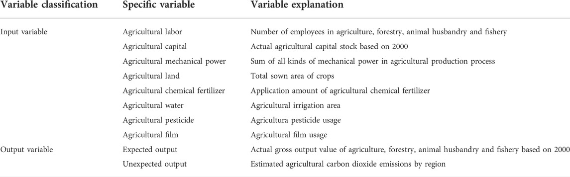
TABLE 1. Input-output variables of ALEE.

3.3.1 Input indicators

(1) Agricultural labor. Agricultural labor is expressed by the number of employees in agriculture, forestry, animal husbandry and fishery (10,000 individuals).

(2) Agricultural capital. Based on previous research (Li et al., 2021; Liu and Yang, 2021), the “perpetual inventory method” was used to calculate the capital stock. The calculation formula is$K_{i,t}=I_{i.t}+\left(1-\delta \right)K_{i,t-1}$. Where$K_{i,t}$ is the capital stock of the $i$-th province during the $t$-th period,$I_{i,t}$ is the investment of $i$-th province in $t$-th period. $\delta$represents the depreciation rate.

(3) Agricultural mechanical power: Agricultural mechanical power is expressed by the total power of agricultural machinery (10,000 kW).

(4) Agricultural land. Agricultural land is expressed by the total planting area of crops (1000 HA)

(5) Agricultural chemical fertilizer. Agricultural chemical fertilizer is expressed by the net amount of agricultural chemical fertilizer application (10,000 tons).

(6) Agricultural pesticide. Agricultural pesticide is expressed by the use amount of pesticide (10,000 tons).

(7) Agricultural film. Agricultural film is expressed in tons of agricultural film.

(8) Agricultural water. Agricultural water is expressed in effective irrigation area (1,000 ha).

3.3.2 Output indicators

(1) Expected output: Expected output is represented by gross agricultural output value (100 million yuan). In this paper, the total output value of agriculture, forestry, animal husbandry and fishery based on 2000 (that is, the general agricultural output value) was taken as the expected output of agriculture.

(2) Unexpected output: Unexpected output is characterized by agricultural carbon emissions (10,000 tons). This paper adopted the calculation method in the 2007 National Greenhouse Gas Inventory Guidelines compiled by IPCC (Solomon, 2007), and the calculation formula is as follows:

$E=\sum e_i=\sum (T_i\times {\delta }_i)(9)$

In the formula, $E$represents the agricultural total carbon emission. $e_i$represents the carbon emission from carbon emission sources$i$. $T_i$ represents the consumption of carbon emission sources$i$. ${\delta }_i$ represents the carbon emission coefficient of carbon emission sources$i$. In this study, nine kinds of agricultural production data were used to calculate CO₂ emissions, and the related parameter values are shown in Table 2.

TABLE 2

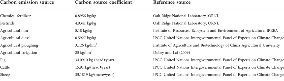
TABLE 2. Carbon emission coefficient of agricultural carbon emission sources.

3.3.3 Indicators of influencing factors

A variety of factors, including economy, society, technology, and system, will have a significant impact on the low-carbon economic efficiency. Based on previous research, this paper concluded that seven factors will influence ALEE: Economic growth level (X1), Capital deepening degree (X2), Agricultural scientific and technological progress (X3), Government fiscal expenditure (X4), Agricultural planting structure (X5), Rural electricity consumption (X6) and Agricultural disaster (X7). The explanations of specific factors are shown in Table 3.

(1) Economic growth level (X1): The scale of regional agricultural output and the agricultural technological progress are directly influenced by the level of agricultural economic development, which has a significant impact on agricultural production efficiency (Liu et al., 2021). The continuous improvement of economic development level can provide the necessary material and technical foundation for environmental improvement, especially in the face of declining ecological capital and more stringent resource and environmental constraints. This variable was expressed using per capita gross agricultural output value in this paper.

(2) Capital deepening degree (X2): The inflow of social capital into agriculture has resulted in the decrease of agricultural labor force, the increase of the agricultural capital-to-labor-force ratio, and the deepening of agricultural capital. On the one hand, capital deepening solved the problem of insufficient agricultural investment and promoted agricultural development. On the other hand, because of the low production capacity of China’s agriculture, it was insufficient to absorb the increasing capital investment, and some enterprises blindly followed the trend of investment, leading to capital waste and reducing agricultural productivity. This variable was expressed using per capita agricultural fixed capital investment in this paper.

(3) Agricultural science and technology progress (X3): Since the reform and opening up, China has made significant investments in agricultural technology research, development, and application. It also learned advanced technology and management concepts from other developed countries. Agricultural science and technology advanced at a rapid pace, and significant contributions to agricultural development was made by effectively improving agricultural production capacity. China’s agriculture has recently entered a critical transition period from traditional to green, ecological, and low-carbon modern agriculture. Agricultural scientific and technological advancement can significantly improve the utilization rate of resources and provide significant impetus for the sustainable and healthy development of agriculture. Advances in agricultural science and technology are helping to improve the ALEE. This variable was expressed using the ratio of internal R&D expenditure to GDP in this paper.

(4) Government fiscal expenditure (X4): Fiscal expenditure, as a form of government intervention, has a significant regulatory effect on agricultural carbon emissions. The greater the government expenditure on the agricultural sector, the more attention the government attaches to agricultural development. However, government expenditure, on the other hand, has a “double-edged sword” effect on agricultural carbon emission performance. The government fiscal support is conducive to improving the level of agricultural production, which is inextricably linked to the promotion of new agricultural varieties, the construction of rural facilities, and agricultural technological progress. On the other hand, excessive fiscal expenditure will disrupt the agricultural market, negating the important role of the market in the allocation of agricultural resources and lowering agricultural capital productivity. Furthermore, increased agricultural fiscal expenditure will increase agricultural consumption of chemical fertilizers, pesticides, and other production methods, resulting in an increase in carbon emissions. Government fiscal expenditure was represented in this paper by the proportion of agricultural, forestry, and water affairs fiscal expenditure to total fiscal expenditure.

(5) Agricultural planting structure (X5): Planting structure has a significant impact on agricultural production efficiency, because it dominates the entire agricultural sector. Planting is generally divided into two categories: food crops and cash crops. Food crops require more agricultural means of production than cash crops, so the level of intensification is low, as is the value generated per unit cultivated land area. The greater the proportion of food crops in the overall planting industry, the less likely it is to improve ALEE. This variable was expressed using the ratio of sown area of food crops to total sown area of crops in this paper.

(6) Rural electricity consumption (X6): Electricity is a critical energy for agricultural production. Compared with other fossil fuels such as diesel, electricity is classified as secondary energy. Large-scale electricity use can effectively reduce agricultural diesel consumption, which has a positive impact on lowering carbon emissions and protecting the agricultural environment. To eliminate the possible influence of collinearity, the natural logarithm of rural electricity consumption by region was used to represent rural electricity consumption in this paper.

(7) Agricultural disaster (X7): Because of China’s delayed agricultural modernization, poor agricultural infrastructure, and relatively backward agricultural production methods, agricultural production is more vulnerable to natural disasters than other industrial sectors. Natural disasters will reduce or even cause the failure of agricultural crops, reducing the scale of agricultural output. The reduction of agricultural output obviously has a negative impact on ALEE. The natural logarithm of crop disaster area was used as a substitute variable for agricultural disaster in this paper.

TABLE 3

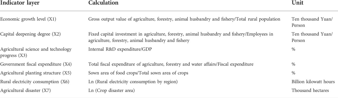
TABLE 3. Indicators of influencing factors of ALEE.

3.4 Data sources

Considering the availability and comprehensiveness of data, the sample includes data from 31 provinces in China from 2000 to 2018. Tibet, Hongkong, Macau and Taiwan are excluded because of the serious lack of data. The data of Agricultural labor, Agricultural machinery power, Agricultural chemical fertilizer, Agricultural pesticides, Agricultural film, Gross agricultural output value, Gross agricultural output value index, Sown area of crops, Total rural population, Rural electricity consumption, and Crop disaster area were from the China Rural Statistical Yearbook (2001–2019). GDP, Fixed capital investments in agriculture, forestry, animal husbandry and fishery, Fixed capital investments price index, agricultural irrigation area, sown area of crops, Total fiscal expenditure of agriculture, forestry and water affairs, Total fiscal expenditure were from China Statistical Yearbook (2001–2019). Internal R&D expenditure data were from China Statistical Yearbook of Science and Technology (2001–2019). Other data were from Local Statistical Yearbooks. In addition, the source of carbon emission coefficient is shown in Table 2.

4 Empirical results and analysis

4.1 Time series evolution characteristics of china’s ALEE

All input-output variables were incorporated into the MaxDEA software based on Eqs. 1–3. After running, the ALEE of each province was calculated.

(1) From the perspective of regions (Figure 1A), ALEE differences are obvious. The ALEE of the eastern region is substantially higher than that of the central and western regions, with the central efficiency being the lowest. This is due to the significant disparity in natural endowments and resource allocation between regions. The eastern region has many advantages in both economic and technological development. It can be further seen that the overall fluctuation trend is basically the same. ALEE of China and the three regions all experience a “L” type trend of decline first and then stability.

FIGURE 1

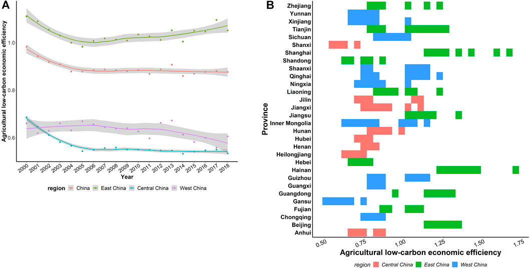
FIGURE 1. (A) shows the average agricultural low-carbon economic efficiency in East China, Central China, West China and China. (B) Shows the distribution of agricultural low-carbon economic efficiency in the provinces.

In the first stage (2000–2005), China vigorously developed agriculture and placed a high value on improving agricultural production technology. However, the agricultural production mode was still fairly traditional, with high input, high consumption, and high emissions. More carbon emissions were produced while the agricultural economy improved, resulting in a downward trend of ALEE in the whole country and the eastern, central, and western regions.

During the second stage (2006–2018), “agriculture, rural areas and farmers” had been the theme of the No. 1 central document. Environmental issues in China gradually received attention. The government issued a series of policies to encourage the development of low-carbon agriculture. And the work of reducing agricultural CO₂ emissions was carried out in stages. At the same time, China introduced many advanced technologies from developed countries. In this context, agricultural carbon emissions decreased to some extent. However, due to the agricultural system and resource endowment, China’s agriculture was still dominated by small farmers, which has a negative impact on growth in many ways (Cassidy and McGrath, 2015; Ji et al., 2016), resulting in ALEE of China and the three regions not growing significantly.

The result is inconsistent with prior research on China’s agricultural productivity considering environmental restrictions. Most research revealed China’s agricultural green total factor efficiency has been increasing in the past few years. (Liu et al., 2021; Han et al., 2018). Similarly, agriculture ecological efficiency is gradually increasing in most studies (Chi et al., 2022; Liu et al., 2020). This may be because the ALEE index we use has stricter restrictions on the environment. China is still implementing traditional agriculture today, which has resulted in substantial carbon emissions and significant environmental harm from national intensive agricultural production. It will take more time to significantly enhance ALEE, despite the fact that China has formulated and implemented many energy-saving and carbon emission reduction strategies in the agriculture sector.

(2) In terms of provinces (Figure 2B), there are significant differences in ALEE among provinces. Most eastern provinces are more efficient, at around 1. Hainan, Shanghai, Beijing, Guangdong, Jiangsu and Tianjin all reach the forefront of production. In addition, Hainan and Shanghai are in a leading position in efficiency. In the central and western provinces, ALEE in central and western provinces is far lower than that in eastern provinces, and there are significant differences between provinces. ALEE in Shaanxi is in the forefront of production, while the efficiency of Heilongjiang, Gansu, and Shanxi is at the bottom, with the value that is not even half of Shaanxi.

FIGURE 2

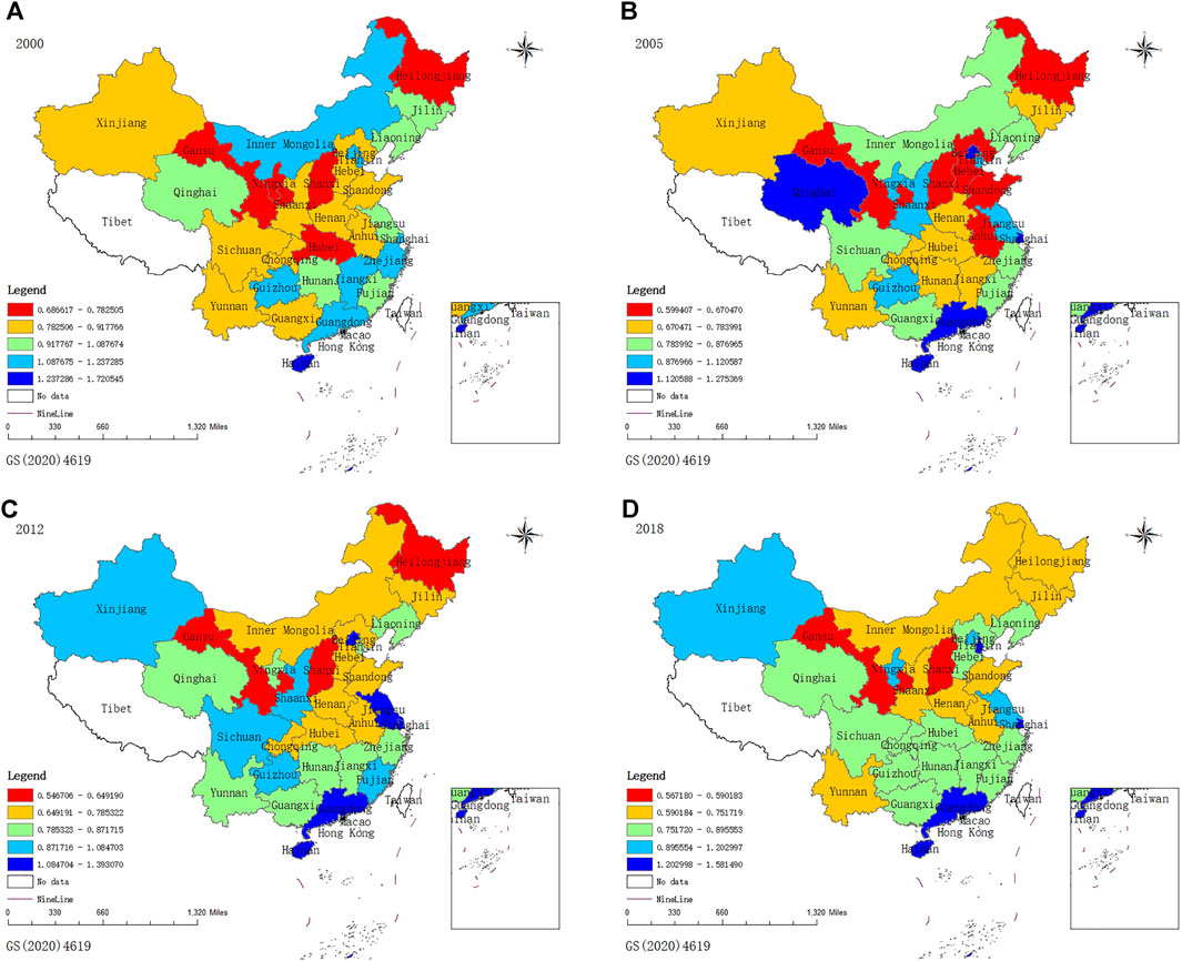
FIGURE 2. (A) shows the agricultural low-carbon economic efficiency in each province in 2000; (B) shows the agricultural low-carbon economic efficiency in each province in 2005; (C) shows the agricultural low-carbon economic efficiency in each province in 2012; (D) shows the agricultural low-carbon economic efficiency in each province in 2020.

4.2 Spatial differentiation characteristics of ALEE

To more intuitively observe the spatial distribution characteristics of ALEE in each province, ArcGIS 10.7 was used to graphically display the ALEE in China for four representative years: 2000, 2005, 2012, and 2018, as shown in Figure 2. Overall, ALEE differs substantially between the east, center, and west, with high-efficiency provinces clustered in the east and low-efficiency provinces concentrated in the central and western regions.

ALEE of Hainan, Shanghai, Beijing, Guangdong, Jiangsu, and Tianjin in the eastern region is at the forefront of China all year. Hainan has a distinct advantage over other provinces due to its unique geographical location and stunning natural environment. As a large province with good ecological environment, Hainan vigorously develops ecological and sightseeing agriculture, thereby creating a favorable environment for the development of low-carbon agriculture. Shanghai, Beijing, Guangdong, Jiangsu, and Tianjin all have high ALEE, which is linked to their favorable geographic location, particularly the growth of suburban agriculture. However, ALEE in Hebei and Shandong is relatively poor. They are even less than 0.7 in 2005. This could be because their agricultural production structure is largely a crop-based agricultural province in China.

In general, ALEE of central region is not ideal. Heilongjiang and Shanxi’s ALEE is always at the bottom of the country. As a major grain producing area in China, the planting structure with most food crops and few cash crops limits the low-carbon development of agriculture in Heilongjiang. Shanxi’s agricultural production suffers from poor innate conditions and unreasonable agricultural industrial structure. Shanxi is a major energy province in China, with high energy consumption. Furthermore, the ALEE of other central provinces, such as Anhui, Jilin, Henan, Jiangxi, Hubei, and Hunan, is high but needs to be further improved in the future.

ALEE is quite different in western provinces. Yunnan and Gansu, in particular, have low ALEE. In Guangxi, Qinghai, Ningxia, and Xinjiang, ALEE is high and growing, while in Inner Mongolia it shows a downward trend. Chongqing, Sichuan, Guizhou, and Shaanxi’s ALEE is well overall during the study period, but it is not consistent. This contradicts previous research, which found that provinces with higher economic development also perform better in agricultural green production, while provinces with lower economic development perform worse (Pang et al., 2016; Yang et al., 2018). This demonstrates that provinces with low economic performance can still improve their low-carbon efficiency in other ways. For example, a series of subsidy policies and technology introductions implemented by the Chinese government in recent years have helped Xinjiang improve ALEE.

4.3 Spatial correlation analysis of ALEE

As shown in Table 4, this paper used Geoda software to calculate Global Moran’s I of China’s ALEE, based on Eqs. 4, 5. The Global Moran’s I values of China’s ALEE are all positive, as shown in Table 4. Except for a few years (2004), other years all pass the test of 10%, 5%, or 1% of the significant level. The findings show a significant positive spatial correlation between China’s ALEE and geographical location. At the same time, it implies that ALEE exhibits spatial agglomeration rather than randomness in spatial distribution. In other words, neighboring provinces’ ALEE has a strong imitation effect. This spatial effect must be considered in the empirical study of the influencing factors of ALEE. Otherwise, the empirical results may be significantly skewed.

TABLE 4

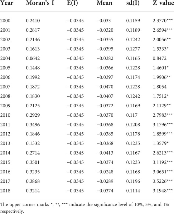
TABLE 4. Global Moran’s I of ALEE.

To further explore the local spatial agglomeration characteristics of ALEE in provinces in China, Moran scatter plot was further drawn. As shown in Figure 3, then the spatial correlation of ALEE was analyzed by ArcGIS, based on calculating Moran’s I index of ALEE in various provinces.

FIGURE 3

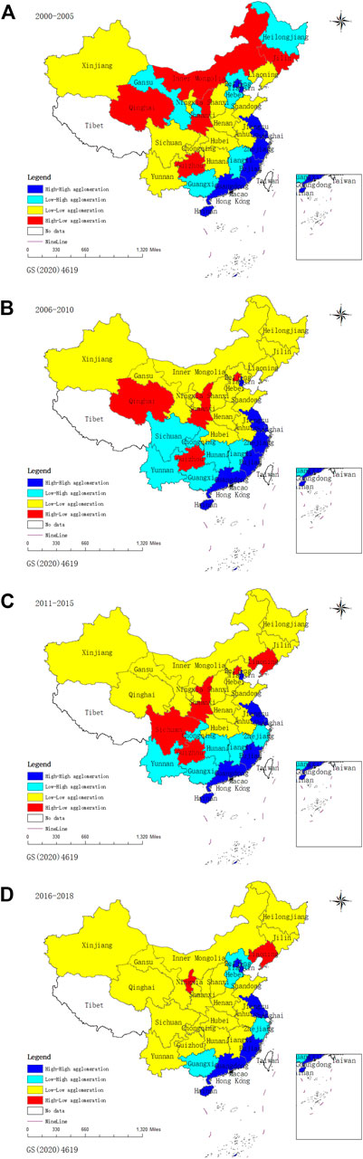
FIGURE 3. (A) shows Spatial autocorrelation of agricultural low-carbon economic efficiency in China from 2000 to 2005; (B) shows Spatial autocorrelation of agricultural low-carbon economic efficiency in China from 2006 to 2010; (C) shows Spatial autocorrelation of agricultural low-carbon economic efficiency in China from 2011 to 2015; (D) shows Spatial autocorrelation of agricultural low-carbon economic efficiency in China from 2016 to 2018.

In general, ALEE shows significant spatial agglomeration characteristics from 2000 to 2018, primarily characterized by H-H agglomeration and L-L agglomeration, indicating that ALEE in this region is similar to that of adjacent regions. In addition, the spatial agglomeration characteristics of ALEE are improved during the sample period. More provinces appear L-L agglomeration in 2018. These provinces have low ALEE, as do surrounding provinces. This clearly demonstrates that ALEE is spatially dependent among provinces, while spatial heterogeneity is weakened.

Specifically, Hainan, Jiangsu, Beijing, Guangdong and Shanghai are the provinces with H-H concentration, owing to their favorable geographic location and abundant agricultural resources. Sichuan, Chongqing, Shandong, Shaanxi, Henan, Hubei, Shanxi, and Yunnan always show L-L agglomeration in the sample period. Furthermore, the number of provinces with L-L agglomeration is growing. Most provinces show L-L agglomeration between 2016 and 2018, indicating that China’s ALEE has not been improved significantly.

5 Spatial econometric analysis of influencing factors of ALEE

5.1 Results of spatial economic model

In this paper, the traditional least square method was used to first simulate the model of influencing factors of ALEE, and then Matlab7.12 software was used to further verify whether the residual term of the model has spatial autocorrelation, providing a foundation for the adoption of a spatial econometric model. Only estimation results can be obtained by using OLS. Because it fails to account for serial correlations in the efficiency score. Then, it requires a restrictive separability condition between the input-output space and the environmental factors space. The separability condition means that the exogenous variables do not exert any effect on the frontier of full efficiency, but may influence only the distribution of the efficiency scores (Badin et al., 2010).

The specific regression results are shown in Table 5, which provides estimation results for four different models, namely no fixed, spatial fixed, time fixed, and bidirectional fixed, to demonstrate that controlling the fixed effect can improve model estimation accuracy. The advantages and disadvantages of each model are judged by comparing the parameters of four different models, and the model with the strongest explanation is chosen.

TABLE 5

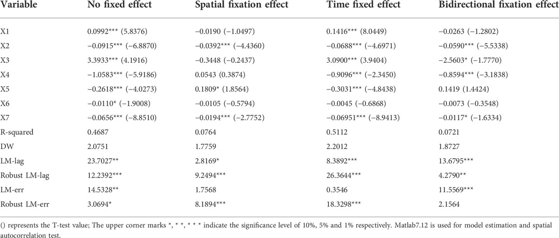
TABLE 5. Estimation and test results of common panel data model.

Firstly, the goodness of fit judgment coefficients of the four models are compared. Compared with the other three models, the R-squared value of the time fixed effect model is the highest, which is 0.5112. Therefore, the fitting degree of time fixed effect is the best. Secondly, compared with the other three models, the DW value of time fixed effect is also the highest, which is 2.2012. After the above comparison, it is found that the time fixed effect performs best in both R-squared value and DW value. Therefore, the time fixed effect model is the most suitable choice for this empirical model. At the same time, the second half of Table 6 examines whether the residual term of the model has spatial autocorrelation. The results show that the LM-lag value of the time-fixed effect model is 8.3892, which is significant at the 1% level, but the LM-err value fails to pass the test the significant level. The results confirm that the residual term of the general model has significant spatial autocorrelation, which contradicts the premise that the explained variables of the general model are independent of each other. Therefore, there may be some deviation in the estimation results of the model. In this case, spatial metrology is required to correct the results of the traditional model. Furthermore, since LM-lag is clearly superior to LM-err, the spatial autoregressive model is more appropriate for this paper than the spatial error model.

TABLE 6

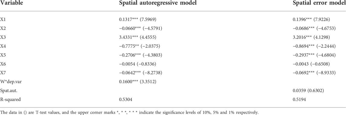
TABLE 6. Estimation and test results of spatial econometric model (Time fixed effect).

Since the estimation results of the traditional model cannot avoid spatial autocorrelation of the residual term, this paper re-estimated the model using Eqs. 7, 8. Table 6 displays the specific estimation results of the spatial model. The spatial lag term W*dep.var in the spatial autoregressive model is 0.1600 and passes the 1% significant level test. However, the spatial error term Spat. aut. In the spatial error model is not significant, as shown in Table 6. This result demonstrates the rationality of spatial econometric model again. The R-squared values of the spatial models are all higher than those of common models in Table 6, indicating that the models’ fitting degree is improved further. Furthermore, the T-test values of some variable coefficients in the spatial econometric model are improved, indicating that the estimation result is optimized on the basis of common model. Furthermore, compared with the spatial error model, the R-squared value of the spatial autoregressive model is higher, implying that the explanatory power of the model is stronger. By contrast, the estimation results of the spatial autoregressive model were finally chosen to explain variables in this paper.

5.2 Analysis of influencing factors of ALEE

Economic growth level (X1) has a positive impact on ALEE at a significant level of 1%. That is, while other conditions remain constant, the increase in per capita GDP can promote the improvement of ALEE. As previously stated, the development of the agricultural economy will increase opportunities to contact with advanced agricultural production technologies and promote the improvement of agricultural production efficiency. Furthermore, economic development can generate new concepts of low-carbon development. Implementing the new concept seriously and promoting deep agricultural governance can effectively reduce agricultural carbon emissions and promote low-carbon agriculture development.

The estimated coefficient of Capital deepening degree (X2) is negative, and the test of 1% significance level shows that Capital deepening degree has a negative influence on ALEE. The amount of capital invested in agriculture has increased in recent years, but the existing scale of agricultural production has not been considered, so the amount of capital did not match the scale of agriculture. It was unable to maximize the utility of agricultural capital, resulting in the reduction of the effective allocation rate of agricultural factors.

Agricultural scientific and technological progress (X3) has a positive impact on ALEE at 1% significant level, indicating that increasing the scientific and technological investment is beneficial to improving ALEE. With the increasing investment in science and technology, agricultural green technology innovation was promoted. The combination of agricultural production factors was continuously optimized, thus improving the agricultural production efficiency.

Government expenditure (X4) has a negative impact on ALEE at 5% significant level. In general, increasing government fiscal investment in agriculture can help to improve agricultural production efficiency. However, this is not absolute. Because the investment process may be accompanied by repeated construction, ineffective construction, rent-seeking, and wasteful behavior. Furthermore, low-carbon agriculture is characterized by large investment and slow effect. The large amount of government investment in a short period did not yielded obvious results, but increased agricultural input costs and reduced agricultural production factor allocation efficiency, which has a negative impact on ALEE.

Agricultural planting structure (X5) has a significant negative impact on ALEE. Planting industry is mainly divided into two categories: cash crops and food crops. On the one hand, food crops require more agricultural means of production than cash crops. If the planting structure is unreasonable, the proportion of food crops is too high, which will obviously increase agricultural carbon emissions. On the other hand, massive investment in agricultural means of production not only increases the production cost, but also increases the waste of resources, which has a negative impact on agricultural production efficiency.

The estimated rural electricity consumption coefficient (X6) is negative, but it fails to pass the significant level test, indicating that rural electricity consumption has no significant impact on ALEE. The reason could be that, while increasing the use of electricity helps to reduce agricultural carbon emissions, the high cost of electricity leads to the effect of rural electricity consumption on agricultural low-carbon economic efficiency is not obvious.

Agricultural disaster (X7) has obvious inhibition effect on ALEE. That is, assuming all other conditions remain constant, the larger the affected crop area, the lower ALEE. Crop loss is a direct result of the natural disasters’ impact on agriculture. At the same time, its environmental output is greatly impacted. However, as an unexpected output, agricultural carbon emissions are primarily caused by agricultural inputs and will not be reduced by natural disasters. In this case, ALEE must be affected.

6 Conclusions and policy recommendations

The Super-SBM model was used in this paper to evaluate the ALEE of 31 Chinese provinces from 2000 to 2018. The spatial panel model was used to conduct an empirical study on the influencing factors of ALEE based on the analysis of regional differences and spatial correlation. The conclusions are as follows:

(1) In terms of temporal evolution, ALEE in most provinces shows a downward trend, with only a few provinces improving. ALEE changes in China and the three regions are relatively consistent, exhibiting a clear " L ″ trend of decline first and then stability.

(2) From the spatial differentiation characteristics, provinces in eastern region have higher ALEE, while those in central and western regions have lower ALEE. Hainan’s ALEE has an absolute advantage, while Shanxi is the worst. Only Hainan, Shanghai, Beijing, Guangdong, Jiangsu, Tianjin and Shaanxi’s ALEE is at the forefront of production during the sample period. ALEE in other provinces is not optimal, and there is room for improvement.

(3) ALEE of adjacent provinces in China has a strong imitation effect, and there is a significant positive spatial correlation. China’s ALEE shows obvious spatial agglomeration characteristics of H-H and L-L agglomeration, which are further enhanced over time. The number of L-L agglomeration provinces has gradually increased, indicating that China’s ALEE has not been improved significantly.

(4) From the perspective of influencing factors, Economic growth level and Agricultural scientific and technological progress play an important role in promoting ALEE. However, Capital deepening degree, Government fiscal expenditure, Agricultural planting structure, and Agricultural disaster have significant inhibitory effects on ALEE. Rural electricity consumption has a negative impact, but it is not statistically significant.

In addition to the above research findings, this paper also makes the following policy recommendations to promote the development of low-carbon agriculture in China:

(1) To avoid policy convergence and blind duplication, all localities should consider their current situation. It is necessary to develop low-carbon agriculture in accordance with local conditions. The eastern region should continue to maximize its own advantages by not only focusing on its own modern agricultural development and technological innovation, but also strengthening exchanges and sharing experiences with the central and western regions. Central and western regions should actively develop distinctive agricultural industries, learn advanced management methods and technology from the eastern regions.

(2) Taking the implementation of rural revitalization strategy as an opportunity to expand the agricultural economy. On the one hand, economic growth can promote the transformation of traditional agriculture into new modern agriculture with low energy consumption, pollution, and emissions. On the other hand, low-carbon agriculture can become a new economic growth point of rural revitalization and comprehensively promote the modernization process of agricultural production.

(3) R&D of agricultural low-carbon production technology should be strengthened. Enterprises should be encouraged to participate in agricultural technological innovation and improve the conversion rate of agricultural technological achievements. The government should not only prioritize the R&D of agricultural ecological carbon sequestration technology, but also put it into practice as soon as possible.

(4) Agricultural carbon emissions can be effectively controlled from the source by reducing traditional agricultural inputs such as chemical fertilizers, pesticides, and agricultural films, and continuously improving the treatment level of waste resources. At the same time, organic fertilizer can be promoted to improve the recycling rate of chemical fertilizer. Furthermore, studies on the composition ratio of poultry feed can reduce the intake of substances that may cause carbon emissions

(5) The original agricultural industrial structure is no longer capable of meeting the demands of regional growth. Agricultural industrial structure must be further adjusted and optimized, as well as new division of labor and scientific layout. To promote green, healthy, and ecological breeding, the structure should be adjusted to avoid blind duplication. All localities should rationally divide the planting structure and breeding density according to their own conditions and agricultural development needs.

(6) The efficiency of government public investment should be improved and a long-term low-carbon agricultural development mechanism should be created. Some adjustments should be made to the current agricultural subsidy policy. The government needs to make rational use of funds and put forward some targeted fiscal policies.

Data availability statement

The original contributions presented in the study are included in the article/Supplementary Material; further inquiries can be directed to the corresponding author.

Author contributions

DM: Conceptualization, Methodology, Software, Resources, Writing—review and editing, Funding acquisition. YaX: Supervision, Writing—review and editing, Visualization, Funding acquisition. FZ: Resources, Investigation. NZ: Writing—review and editing, Funding acquisition. YuX: Visualization. XC: Resources.

Funding

This research was jointly funded by the Chongqing Social Science Planning Youth Project “Incentive Mechanism and Optimization Countermeasures for Green Development of Chongqing Construction Industry” (Grant 2020QNGL38); and Graduate Innovation Project of Chongqing University of Technology “Study on the Development of Agricultural Low Carbon Economy in the Yangtze River Economic Belt under the Background of Rural Revitalization” and “Study on the Comprehensive Measurement, Spatio-temporal Evolution and Upgrading Path of the High-quality Development Level of the Logistics Industry in the Yangtze River Economic Belt (No. gzlcx20223124, gzlcx20223114).

Acknowledgments

We are particularly grateful for the financial support from the project and we are grateful to reviewers and editors for their comments and suggestions on this paper.

Conflict of interest

The authors declare that the research was conducted in the absence of any commercial or financial relationships that could be construed as a potential conflict of interest.

Publisher’s note

All claims expressed in this article are solely those of the authors and do not necessarily represent those of their affiliated organizations, or those of the publisher, the editors and the reviewers. Any product that may be evaluated in this article, or claim that may be made by its manufacturer, is not guaranteed or endorsed by the publisher.

Reference

Adetutu, M. O., and Ajayi, V. (2020). The impact of domestic and foreign R&D on agricultural productivity in sub-Saharan Africa. World Dev. 125, 104690. doi:10.1016/j.worlddev.2019.104690

CrossRef Full Text | Google Scholar

Anselin, L. (1988). Spatial econometrics: methods and models. Netherlands: Kluwer Academic Publishers.

Google Scholar

Badin, L., Daraio, C., and Simar, L. (2010). Optimal bandwidth selection for conditional efficiency measures: a data-driven approach. Eur. J. Oper. Res. 201, 633–640. doi:10.1016/j.ejor.2009.03.038

CrossRef Full Text | Google Scholar

Bai, C., Du, K., Yu, Y., and Feng, C. (2019). Understanding the trend of total factor carbon productivity in the world: insights from convergence analysis. Energy Econ. 81, 698–708. doi:10.1016/j.eneco.2019.05.004

CrossRef Full Text | Google Scholar

Benedetti, I., Branca, G., and Zucaro, R. (2019). Evaluating input use efficiency in agriculture through a stochastic frontier production: an application on a case study in apulia(Italy). J. Clean. Prod. 236, 117609. doi:10.1016/j.jclepro.2019.117609

CrossRef Full Text | Google Scholar

Cao, X. C., Zeng, W., Wu, M. Y., Guo, X. P., and Wang, W. G. (2020). Hybrid analytical framework for regional agricultural water resource utilization and efficiency evaluation. Agric. Water Manag. 231, 106027. doi:10.1016/j.agwat.2020.106027

CrossRef Full Text | Google Scholar

Cassidy, A., and McGrath, B. (2015). Farm, place and identity construction among Irish farm youth who migrate. J. Rural. Stud. 37, 20–28. doi:10.1016/j.jrurstud.2014.11.006

CrossRef Full Text | Google Scholar

Charnes, A., Cooper, W. W., and Rhodes, E. (1978). Measuring the efficiency of decision making units. Eur. J. Oper. Res. 2 (6), 429–444. doi:10.1016/0377-2217(78)90138-8

CrossRef Full Text | Google Scholar

Chen, Y., Miao, J., and Zhu, Z. (2021). Measuring green total factor productivity of China's agricultural sector: A three-stage SBM-DEA model with non-point source pollution and CO₂ emissions. J. Clean. Prod. 318, 128543. doi:10.1016/j.jclepro.2021.128543

CrossRef Full Text | Google Scholar

Chi, M., Guo, Q., Mi, L., Wang, G., and Song, W. (2022). Spatial distribution of agricultural eco-efficiency and agriculture high-quality development in China. Land 11 (5), 722. doi:10.3390/land11050722

CrossRef Full Text | Google Scholar

Chopra, R., Magazzino, C., Shah, M. I., Sharma, G. D., Rao, A., and Shahzad, U. (2022). The role of renewable energy and natural resources for sustainable agriculture in ASEAN countries: Do carbon emissions and deforestation affect agriculture productivity? Resour. Policy 76, 102578. doi:10.1016/j.resourpol.2022.102578

CrossRef Full Text | Google Scholar

Cui, Y., Khan, S. U., Deng, Y., and Zhao, M. J. (2021). Regional difference decomposition and its spatiotemporal dynamic evolution of Chinese agricultural carbon emission: considering carbon sink effect. Environ. Sci. Pollut. Res. 28 (29), 38909–38928. doi:10.1007/s11356-021-13442-3

CrossRef Full Text | Google Scholar

Department for Business Innovation and Skills (DBIS) (2015). The size and performance of the UK low carbon economy: Report for 2010 to 2013. Available at: https://www.gov.uk/government/publications/low-carbon-economy-size-and-performance (Accessed March 24, 2015).

Google Scholar

Diao, P., Zhang, Z., and Jin, Z. (2018). Dynamic and static analysis of agricultural productivity in China. China Agric. Econ. Rev. 10 (2), 293–312. doi:10.1108/CAER-08-2015-0095

CrossRef Full Text | Google Scholar

Dubey, A., and Lal, R. (2009). Carbon footprint and sustainability of agricultural production systems in Punjab, India, and Ohio, USA. J. Crop Improv. 23 (4), 332–350. doi:10.1080/15427520902969906

CrossRef Full Text | Google Scholar

Emrouznejad, A., and Yang, G. (2018). A survey and analysis of the first 40 years of scholarly literature in DEA: 1978–2016. Socioecon. Plann. Sci. 61, 4–8. doi:10.1016/j.seps.2017.01.008

CrossRef Full Text | Google Scholar

Geng, Q. L., Ren, Q. F., Nolan, R. H., Wu, P. T., and Yu, Q. (2019). Assessing China's agricultural water use efficiency in a green-blue water perspective: A study based on data envelopment analysis. Ecol. Indic. 96, 329–335. doi:10.1016/j.ecolind.2018.09.011

CrossRef Full Text | Google Scholar

Haining, R. (1993). Spatial data analysis in the social and environmental sciences. England: Cambridge University Press.

Google Scholar

Hamid, S., and Wang, K. (2022). Environmental total factor productivity of agriculture in south asia: A generalized decomposition of luenberger-hicks-moorsteen productivity indicator. J. Clean. Prod. 351, 131483. doi:10.1016/j.jclepro.2022.131483

CrossRef Full Text | Google Scholar

Han, H. B., Zhong, Z. Q., Wen, C. C., and Sun, H. G. (2018). Agricultural environmental total factor productivity in China under technological heterogeneity: characteristics and determinants. Environ. Sci. Pollut. Res. 25, 32096–32111. doi:10.1007/s11356-018-3142-4

PubMed Abstract | CrossRef Full Text | Google Scholar

He, R., Shao, C. F., Shi, R. G., Zhang, Z. Y., and Zhao, R. (2020). Development trend and driving factors of agricultural chemical fertilizer efficiency in China. Sustainability 12 (11), 4607. doi:10.3390/su12114607

CrossRef Full Text | Google Scholar

Hu, Y., Liu, X., Zhang, Z., Wang, S., and Zhou, H. (2022). Spatiotemporal heterogeneity of agricultural land eco-efficiency: A case study of 128 cities in the Yangtze River basin. Water 14 (3), 422. doi:10.3390/w14030422

CrossRef Full Text | Google Scholar

Huang, W., and Jiang, L. (2019). Efficiency performance of fertilizer use in arable agricultural production in China. China Agr. Econ. Rev. 11 (1), 52–69. doi:10.1108/CAER-12-2017-0238

CrossRef Full Text | Google Scholar

Huang, X., Xu, X., Wang, Q., Zhang, L., Gao, X., and Chen, L. (2019). Assessment of agricultural carbon emissions and their spatiotemporal changes in China, 1997–2016. Int. J. Environ. Res. Public Health 16 (17), 3105. doi:10.3390/ijerph16173105

PubMed Abstract | CrossRef Full Text | Google Scholar

Huang, X., Feng, C., Qin, J., Wang, X., and Zhang, T. (2022). Measuring China's agricultural green total factor productivity and its drivers during 1998-2019. Sci. Total Environ. 829, 154477. doi:10.1016/j.scitotenv.2022.154477

PubMed Abstract | CrossRef Full Text | Google Scholar

Solomon, S. (2007). IPCC (2007): Climate change the physical science basis. In Agu fall meeting abstracts 2007, U43D-01. Available at: https://ui.adsabs.harvard.edu.

Google Scholar

Ji, X. Q., Rozelle, S., Huang, J. K., Zhang, L. X., and Zhang, T. L. (2016). Are China's farms growing? China World Econ. 24 (1), 41–62. doi:10.1111/cwe.12143

CrossRef Full Text | Google Scholar

Kay, S., Rega, C., Moreno, G., den Herder, M., Palma, J., Borek, R., et al. (2019). Agroforestry creates carbon sinks whilst enhancing the environment in agricultural landscapes in Europe. Land Use Policy 83, 581–593. doi:10.1016/j.landusepol.2019.02.025

CrossRef Full Text | Google Scholar

Kim, D. G., Kirschbaum, M., and Beedy, T. L. (2016). Carbon sequestration and net emissions of CH₄ and N₂O under agroforestry: Synthesizing available data and suggestions for future studies. Agric. Ecosyst. Environ. 226, 65–78. doi:10.1016/j.agee.2016.04.011

CrossRef Full Text | Google Scholar

Li, H., Luo, L., Zhang, X., and Zhang, J. (2021). Dynamic change of agricultural energy efficiency and its influencing factors in China. Chin. J. Popul. Resour. Environ. 19 (4), 311–320. doi:10.1016/j.cjpre.2022.01.004

CrossRef Full Text | Google Scholar

Li, Y. (2014). Study on agricultural carbon sink function and compensation mechanism-taking alimentarn crop as an example. Shandong: Shandong Agricultural University. (Ph.D. Dissertation).

Google Scholar

Liu, Y., and Feng, C. (2019). What drives the fluctuations of “green” productivity in China's agricultural sector? A weighted russell directional distance approach. Resour. Conserv. Recycl. 147, 201–213. doi:10.1016/j.resconrec.2019.04.013

CrossRef Full Text | Google Scholar

Liu, M., and Yang, L. (2021). Spatial pattern of China’s agricultural carbon emission performance. Ecol. Indic. 133, 108345. doi:10.1016/j.ecolind.2021.108345

CrossRef Full Text | Google Scholar

Liu, Y., Zou, L., and Wang, Y. (2020). Spatial-temporal characteristics and influencing factors of agricultural eco-efficiency in China in recent 40 years. Land Use Policy 97, 104794. doi:10.1016/j.landusepol.2020.104794

CrossRef Full Text | Google Scholar

Liu, D., Zhu, X., and Wang, Y. (2021). China’s agricultural green total factor productivity based on carbon emission: an analysis of evolution trend and influencing factors. Clean. Prod. 278, 123692. doi:10.1016/j.jclepro.2020.123692

CrossRef Full Text | Google Scholar

Pang, J., Chen, X., Zhang, Z., and Li, H. (2016). Measuring eco-efficiency of agriculture in China. Sustainability 8 (4), 398. doi:10.3390/su8040398

CrossRef Full Text | Google Scholar

Ren, Y. J., Peng, Y. L., Campos, B. C., and Li, H. J. (2021). The effect of contract farming on the environmentally sustainable production of rice in China. Sustain. Prod. Consum. 28, 1381–1395. doi:10.1016/j.spc.2021.08.011

CrossRef Full Text | Google Scholar

Rural Social Economic Investigation DivisionNational Bureau of Statistics of China (2018). China rural statistical Yearbook. Beijing: China Statistics Press.

Google Scholar

Shen, Z., Baleˇzentis, T., and Ferrier, G. D. (2019). Agricultural productivity evolution in China: a generalized decomposition of the luenberger-hicks-moorsteen productivity indicator. China Econ. Rev. 57, 101315. doi:10.1016/j.chieco.2019.101315

CrossRef Full Text | Google Scholar

Skevas, I., Emvalomatis, G., and Brümmer, B. (2018). Productivity growth measurement and decomposition under a dynamic inefficiency specification: the case of German dairy farms. Eur. J. Oper. Res. 271 (1), 250–261. doi:10.1016/j.ejor.2018.04.050

CrossRef Full Text | Google Scholar

Toma, P., Miglietta, P. P., Zurlini, G., Valente, D., and Petrosillo, I. (2017). A non-parametric bootstrap-data envelopment analysis approach for environmental policy planning and management of agricultural efficiency in EU countries. Ecol. Indic. 83, 132–143. doi:10.1016/j.ecolind.2017.07.049

CrossRef Full Text | Google Scholar

Wu, H., Guo, S., Guo, P., Shan, B., and Zhang, Y. (2022). Agricultural water and land resources allocation considering carbon sink/source and water scarcity/degradation footprint. J. Sci. Total Environ. 819, 152058. doi:10.1016/j.scitotenv.2021.152058

PubMed Abstract | CrossRef Full Text | Google Scholar

Xiang, H., Wang, Y. H., Huang, Q. Q., and Yang, Q. Y. (2020). How much is the eco-efficiency of agricultural production in west China? Evidence from the village level data. Int. J. Environ. Res. Public Health 17 (11), 4049. doi:10.3390/ijerph17114049

PubMed Abstract | CrossRef Full Text | Google Scholar

Xiong, C., Wang, G., and Xu, L. (2021). Spatial differentiation identification of influencing factors of agricultural carbon productivity at city level in Taihu lake basin, China. Sci. Total Environ. 800, 149610. doi:10.1016/j.scitotenv.2021.149610

PubMed Abstract | CrossRef Full Text | Google Scholar

Xu, J. R., Huang, D. C., He, Z. Q., and Zhu, Y. (2020). Research on the structural features and influential factors of the spatial network of China's regional ecological efficiency spillover. Sustainability 12 (8), 3137. doi:10.3390/su12083137

CrossRef Full Text | Google Scholar

Yang, Z., Wang, D., Du, T., Zhang, A., and Zhou, Y. (2018). Total-factor energy efficiency in China’s agricultural sector: trends, disparities and potentials. Energies 11 (4), 853–916. doi:10.3390/en11040853

CrossRef Full Text | Google Scholar

Yang, W., Zhao, R., Chuai, X., Xiao, L., Cao, L., Zhang, Z., et al. (2019). China’s pathway to a low carbon economy. Carbon Balance Manag. 14 (1), 14–12. doi:10.1186/s13021-019-0130-z

PubMed Abstract | CrossRef Full Text | Google Scholar

Yang, H., Wang, X., and Bin, P. (2022). Agriculture carbon-emission reduction and changing factors behind agricultural eco-efficiency growth in China. J. Clean. Prod. 334, 130193. doi:10.1016/j.jclepro.2021.130193

CrossRef Full Text | Google Scholar

Zhou, Y., Wang, T., Peng, R. C., and Hu, H. M. (2021). Spatial-temporal characteristics and factors of agricultural carbon emissions in the Belt and road region of China. Pol. J. Environ. Stud. 30 (3), 2445–2457. doi:10.15244/pjoes/127414

CrossRef Full Text | Google Scholar