Mid-century change analysis of temperature and precipitation maxima in the Swat River Basin, Pakistan

This study analyzes trends in historical (1989–2018) and projected (2041–2060) temperature and precipitation maxima in the Swat River Basin, Pakistan. This basin has a history of climate-related disasters that directly affected livelihood and personal safety in local communities and are becoming more intense and more frequent due to changing climate. Major economic sources of this basin are agriculture and tourism, both highly sensitive to extreme climate events. Therefore, it is very important to assess future trends in extremes of temperature and precipitation. Non-parametric tests were employed for currently acquired data, while future projections were assessed using the statistical downscaling model (SDSM) with CanESM2 GCM under three scenarios: representative concentration pathways (RCPs) of 2.6, 4.5, and 8.5. The R² value between monthly observed and simulated temperatures varied from 0.82 to 0.91 and 0.92 to 0.96 for training and confirmation periods, respectively. For areal precipitation, an R² value of 0.49 was noted for calibration and 0.35 for validation. Observed temperatures showed a decreasing trend at all stations except Saidu Sharif, but the differences were not significant. Precipitation showed an increasing trend at two stations, Kalam and Malam Jabba, and a decreasing trend at two other stations, Dir and Saidu Sharif. A >2°C rise was noted for the annual projected maximum temperature (2041–2060) at areal and Dir, while Kalam, Malam Jabba, and Saidu Sharif showed a 1°C rise. For precipitation, an approximately 12% increase in annual maximum (areal) and seasonal precipitation (summer and autumn) was seen under all scenarios except RCP 4.5 in which there was a 20% and 32% increase in summer and autumn, respectively. The performance of SDSM in simulating maximum temperature and precipitation was satisfactory.

1 Introduction

Climate change is a continuous and occasionally irreversible movement in the prolonged patterns of atmospheric variables in a particular area and in the whole world (Ikram et al., 2016). The majority of climate experts are of the opinion that climate is varying because of anthropogenic influences and will continue changing unless sufficient mitigation measures are adapted (Anderegg et al., 2010). Climate change is mostly due to variations in the amount of greenhouse gases in the atmosphere (Alexander et al., 2013). This change in the radiative energy budget of the climatic system either by human or natural disturbance is called “climate forcing” or “radiative forcing” (IPCC First assessment report, 1990). Changes in climate forcing affect the quantity and quality of ground water, the frequency and intensity of droughts and floods, and ultimately, the water resource management practices, especially at local scales (Amell, 2003). Thus, studying the effects of climate change on water has been an important area for research and has attained a paramount focus in recent years (Scanlon et al., 2007). From accurate investigations of climate variables measured by weather stations, it is possible to get a clearer picture of how powerful the impacts of climate change are at a regional scale. These trend analysis studies which are normally focused at the country level or in a part of a particular country have been carried out around the globe with outstanding results (Reiter et al., 2012).

By linking hydrological and atmospheric processes, precipitation acts as a critical element of the water cycle (Li et al., 2021) and its variations in terms of floods and droughts have direct effects on water resources and ecosystem services (Wu et al., 2013). The frequency and magnitude of precipitation are strongly linked to changes in climate (Pal and Al-Tabbaa, 2011). Hydrological patterns can be varied mainly by precipitation, which may further influence a society and its environment (Gajbhiye et al., 2016). Hence, accurately predicting precipitation trends is imperative for water resource management and economic development in a region (Ahmad et al., 2018). A warmer atmosphere tends to increase the evaporation rate, leading to more moisture spreading throughout the troposphere which can cause extreme events of precipitation and severe, prolonged droughts (Xu et al., 2006; Zhang et al., 2010). Warming can cause more precipitation as rain rather than snow, which may not only increase flood risks in spring, but also drought probability in summer particularly in snow-fed basins (Trenberth, 2011). Drought accounts for 59% of economic losses caused by climate extremes worldwide (Dong et al., 2022), and Pakistan is facing drought every 6 years and floods every 3 years (Ahmad et al., 2018). Pakistan suffered the worst drought in its history during 1998–2002 and a flood in 2010 due to the greater variability in precipitation in the Upper Indus Basin (Ahmad et al., 2018). Warming of the climate system also affects the sea level by melting snow and ice and thermal expansion of oceans, while increase in the average annual temperature warms the sea surface (IPCC 2007, 2013). The Hindukush glaciers are melting faster and the area will face extreme climatic events (IPCC, 2013). Studies showed that less snow and the recession of glaciers will have a severe impact on downstream areas if warming continues at 0.01°C/year in northern Hindukush areas (Fang et al., 2018).

To address these changes, there is a dire need for qualitative and quantitative evaluation of the impact of climate change on hydrological resources at regional scales. Till now, the general circulation models (GCMs) have been the principal tools for climate projection under various scenarios (Chu et al., 2010). Because of their coarse resolution and ineffectiveness in sorting out prominent features like topography and clouds at sub-grid scales, the current versions of GCMs cannot be directly used for local climate studies (Wilby et al., 2002; Xu et al., 2019). The performance of GCM simulations has been unsatisfactory at regional scales, and to overcome this, downscaling techniques have been developed as tools for connecting atmospheric predictors with local variables. Downscaling can be mainly categorized into dynamic and statistical types. In the dynamic method, the output of a GCM is utilized as the boundary conditions to derive a regional model and local-scale information at a resolution of 5–50 km, which responds in compatible ways to external forcing. However, dynamic downscaling involves high computational costs and mainly relies on GCM boundary conditions. Conversely, statistical downscaling produces regional/station-scale time series by suitable statistical relationships with predictors, which is computationally less expensive, readily transferable, and applicable for evaluation of climate risks. The disadvantage of statistical downscaling is that establishing the appropriate empirical relationships requires collecting data on a sufficiently long timescale (Wilby et al., 2002) of at least 30 years as mentioned in the SDSM user manual (version 4.2). Up to now, there have been certain models, among which the SDSM is prominent and freely available (Wilby et al., 2002). Several studies reported on its ease of use, and its superior capability makes it widely acceptable (Hashmi et al., 2011; Huang et al., 2011; Al-Mukhtar and Qasim, 2019; Saddique et al., 2020).

The study area is highly vulnerable to flooding because of monsoon rain, melting snow and ice, rough terrain, and human-induced factors (Malik and Ahmad, 2014). The area suffered calamitous floods in 1973, 1992, 1993, 1994, 1995, 1996, 2001, 2005, and 2010 (Bahadar et al., 2015). The 2010 flood was highly disastrous in the history of Swat which caused 86 fatalities, damaged 4,000 houses, killed 9,800 head of livestock, destroyed many bridges, and damaged the Amandara as well as the Munda headworks (Rahman and Khan, 2011). Similarly, the river is pivotal for the current and upcoming development of the country, with its three hydroelectric power plants with total capacity of approximately 123 MW, and a future potential of about 1000 MW, which could supply about 25% of the total energy shortage of the country. For that purpose, the government launched the Mohmand Dam project on the same river about 5 km upstream of the Munda headworks. The key objectives of the dam project are flood mitigation, irrigation of 16,737 acres of agricultural land, hydropower generation, and socio-economic uplift of the local people (Sabir et al., 2014). The area is also important for tourism as it is known throughout the country as “eastern Switzerland”. About 38% of the economy of the area relies on tourism and 31% on agriculture, each of which are adversely affected by extreme climatic events. In view of the sensitivity of the lives and livelihoods of the people to climate change and the immense environmental and socio-economic importance of the area, it is crucial to investigate the maximum temperature and precipitation predictions of the area in the context of climate change.

Several studies have been carried out by different researchers like (Archer and Fowler, 2004; Srinivas and Kumar, 2006; Ahmad et al., 2014; Hartmann and Buchanan, 2014; Ahmad et al., 2018; Anjum et al., 2019), but they have discussed only the observed hydro-climatic variables. The novelty of our study lies in the fact that no study has been carried out on the effects of observed and projected maximum temperature and precipitation trends simultaneously in the Swat River Basin. The SDSM using CanESM2 GCM has not been applied, even in the entire Indus Basin; hence this study aims to fill that gap in the research. The objectives of the study are to analyze the trends of observed (1989–2018) maximum temperatures and precipitation and to predict the trends of temperature and precipitation maxima by the middle of this century (2041–2060). The mid-century (near-term) climate projections were chosen because they have been acknowledged as especially significant by policymakers in industry and government, there has been an increase in global research on understanding near-term climate projections, and because of an acceptance of the fact that these climate projections are normally less sensitive to differences between future emission scenarios than long-term projections (IPCC, 2013).

2 Study area

The Swat River is the right bank branch of the Indus River which originates in the high mountains of Swat-Kohistan in northwestern Pakistan. Two rivulets Gabral and Ushu from corresponding glaciers meet at Kalam to form the Swat River. Downstream, it also receives input from perennial streams such as Deolai, Daral, and Harnoi. The Swat River is fed by glaciers, snow, and rain on a north-to-south slope. From Kalam to Mingora, the river runs southward and then turns west until it reaches the greater right-tributary of the Panjkora River. As a whole, the river flows through Kalam, Swat, and Lower Dir, through the districts of Mardan and Malakand and empties into the Kabul River at Nisatta. Seasonally, Swat is affected by the monsoon, altitude, latitude, and the winter wind waves of the Mediterranean Sea. The general climate of the region can be split into sub-humid, humid, and semi-arid (Bahadar et al., 2015). The region is part of the strip influenced by the monsoon and western disturbances with a short mild summer and a long cool winter (Anjum et al., 2016). The warmest month of the year is June with average maximum/minimum temperatures of 33 and 16°C, respectively. The coldest month is January with frequent snowfalls and an average highest and lowest temperature of 11 and −2°C, respectively (Ahmad et al., 2014). The summer season in the area lasts from May till September while winter varies between September and March. The mean precipitation in summer is 246.4 mm and that of winter is 815.3 mm (Khan and Hasan, 2016), while the annual average rainfall fluctuates between 700 mm and 1630 mm (Ahmad et al., 2014). Figure 1 gives details of the study area and Table 1 gives description of the weather stations used in this study.

FIGURE 1

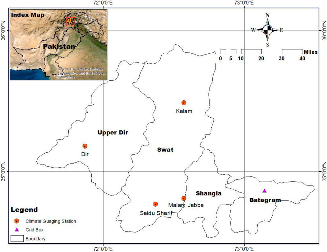
FIGURE 1. Study area map showing the weather stations used in the research.

TABLE 1

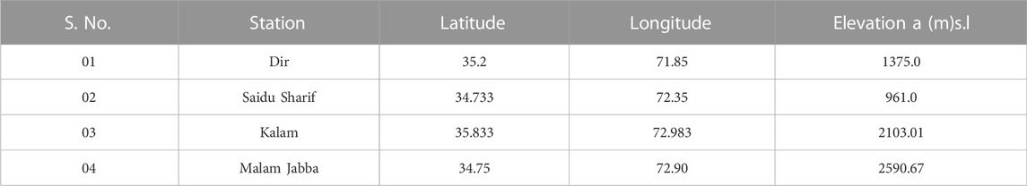
TABLE 1. Details of weather stations used in study.

Swat is positioned almost 160 km northwest of the capital, Islamabad, and is encircled by hills on all sides except the southwest, which offers a channel for the Swat River. To the north of the valley are the Chitral and Ghizar districts, to the east lie Kohistan and Shangla, Malakand and Buner are located in the south, while to the west are the Upper and Lower Dir (Rahman and Khan, 2011). The most prominent vegetation (natural) in the study area is forest composed primarily of conifers in the higher elevations, with patches of weeds and wild species at lower elevations. The area covered by forest is a little larger than the cultivable region. Agriculture, handicrafts and tourism are the chief sources of livelihood. The area is also known for walnuts, citrus fruits, apples, apricot, almonds, and pears (Sultan-i-Rome 2005).

3 Materials and methods

3.1 Data

Historical data of daily temperature and precipitation from 1989 to 2018 at stations in Dir and Saidu Sharif was provided by the Pakistan Meteorological Department in Islamabad, while data of the same time period at the other two stations (Kalam and Malam Jabba) was obtained from the Regional Meteorological Center in Peshawar. This time period was chosen because it had the fewest missing values. There were no missing temperature or precipitation values from the Kalam and Malam Jabba stations. However, some missing values from the Dir and Saidu Sharif stations were extrapolated by taking the mean of the preceding 2 days and the succeeding 2 days (Owolabi et al., 2020). A Pettit test was employed to check the homogeneity of data. The NCEP/NCAR reanalysis dataset downloaded from National Center of Environmental Prediction (https://climate-scenarios.canada.ca/?page=pred-canesm2) was used in this study. It is a daily time series from 1961 to 2005 at a spatial resolution of 2.5° (long.) * 2.5° (lat.) including 26 variables, like mean sea level pressure, near surface relative humidity, 2-m air temperature, near surface specific humidity, etc. The CMIP5-ESMs climate model for high emission (RCP 8.5), intermediate (RCP 4.5), and low emission (RCP 2.6) scenarios at a grid resolution of 2.8125°× 2.8125° was downloaded from the Canadian Centre of Climate Modeling/Analysis for the periods 1961–2005 and 1961–2099. These variables were then used in the SDSM for calibration and validation as well as projection.

3.2 Methods

3.2.1 Trend analysis of the observed data

The basic purpose of trend analysis is to determine whether the observed time series is decreasing, increasing or trendless (Ahmad et al., 2018). A rank-based, non-parametric Mann-Kendall test was used to determine trends in the annual maximum time series of temperature and precipitation. The “null hypothesis” and “alternative hypothesis” implies that the time series is trendless or there is a decreasing/increasing trend, respectively. Since serial correlations affected the results of this test, the trend free “prewhitening” approach of Yue et al. (2002) was used. This technique is widely applied to overcome the effects of autocorrelation and serial correlation. The mathematical equations for calculating MK statistics are given below:

$\mathrm{S}={\displaystyle \sum }_{\mathrm{i}=1}^{\mathrm{m}-1}{\displaystyle \sum }_{\mathrm{j}=\mathrm{i}+1}^{\mathrm{m}}\mathrm{s}\mathrm{g}\mathrm{n}({\mathrm{x}}_{\mathrm{j}}-{\mathrm{x}}_{\mathrm{i}})(1)$

where m represents the observation numbers and x_i and x_j are the ith and jth observations, respectively. The sign function sgn can be calculated by:

$\mathrm{s}\mathrm{g}\mathrm{n}\left({\mathrm{x}}_{\mathrm{j}}-{\mathrm{x}}_{\mathrm{i}}\right)=\left\{\begin{array}{c}1\mathrm{i}\mathrm{f}\left({\mathrm{x}}_{\mathrm{j}}-{\mathrm{x}}_{\mathrm{i}}\right)>0\\ 0\mathrm{i}\mathrm{f}\left({\mathrm{x}}_{\mathrm{j}}-{\mathrm{x}}_{\mathrm{i}}\right)=0\\ -1\mathrm{i}\mathrm{f}\left({\mathrm{x}}_{\mathrm{j}}-{\mathrm{x}}_{\mathrm{i}}\right)<1\end{array}\right.(2)$

The S statistic variance may be calculated as:

$\mathrm{V}\left(\mathrm{S}\right)=\frac{1}{18}\left[\left.\mathrm{m}\left(\mathrm{m}-1\right)\left(2\mathrm{m}+5\right)-{\displaystyle \sum }_{\mathrm{p}=1}^{\mathrm{q}}{\mathrm{t}}_{\mathrm{p}}({\mathrm{t}}_{\mathrm{p}}-1)|(|{2\mathrm{t}}_{\mathrm{p}}|+|5|)\right)\right](3)$

where q denotes tied group numbers while t_p represents the pth group observations. The MK Z statistics can be estimated as:

$\mathrm{Z}=\left\{\begin{array}{c}\frac{\mathrm{S}-1}{\mathrm{V}\left(\mathrm{S}\right)}\mathrm{f}\mathrm{o}\mathrm{r}\mathrm{S}>0\\ 0\mathrm{f}\mathrm{o}\mathrm{r}\mathrm{S}=0\\ \frac{\mathrm{S}+1}{\mathrm{V}\left(\mathrm{S}\right)}\mathrm{f}\mathrm{o}\mathrm{r}\mathrm{S}<0\end{array}\right.(4)$

Another rank-based non-parametric test, Spearman’s rho (Lehmann, 1975; Sneyers, 1990), was used in comparison with the Mann Kendall test. The null hypothesis indicates no trend and the alternative hypothesis means an increasing/decreasing trend over time. The R_sp and Z_sp statistics of the test are defined as following.

${\mathrm{R}}_{\mathrm{s}\mathrm{p}}=1-\frac{6{\displaystyle \sum }_{\mathrm{i}=1}^{\mathrm{n}}{\left({\mathrm{D}}_{\mathrm{i}}-\mathrm{i}\right)}^2}{\mathrm{n}\left({\mathrm{n}}^2-1\right)}(5)$

where D_i denotes the ith observation rank, i indicates the number of the sequential order and n is the complete length of data.

${\mathrm{Z}}_{\mathrm{s}\mathrm{p}}={\mathrm{R}}_{\mathrm{s}\mathrm{p}}\sqrt{\frac{\mathrm{n}-2}{1-{\mathrm{R}}_{\mathrm{s}\mathrm{p}}^2}}(6)$

and Z_sp represents the Student’s t distribution with (n-2) degree of freedom, while negative and positive values of Z_sp correspond to decreasing and increasing trends, respectively. Using the method of Sen (1968), the magnitude of the slope was calculated as:

${\mathrm{b}}_{\mathrm{S}\mathrm{e}\mathrm{n}}=\mathrm{M}\mathrm{e}\mathrm{d}\mathrm{i}\mathrm{a}\mathrm{n}\left[\frac{{\mathrm{Y}}_{\mathrm{i}}-{\mathrm{Y}}_{\mathrm{j}}}{\mathrm{i}-\mathrm{j}}\right]\mathrm{f}\mathrm{o}\mathrm{r}\mathrm{a}\mathrm{l}\mathrm{l}\mathrm{j}<\mathrm{i}(7)$

where Y_i and Y_j denote the data at points (time) i and j, respectively. If the entire number of points in the time-series is n, this implies that $\frac{n\left(n-1\right)}{2}$ and b_Sen will be the estimated slope and median of all slopes, respectively. A negative value of the test describes a decreasing trend, while a positive value shows an increasing trend.

3.2.2 Climate projection and the SDSM

Climate change projection was done with the Canadian Earth System Model Second Generation (CanESM2) developed by the Canadian Centre for Climate Modeling and Analysis which is comprised of the fourth-generation atmospheric general circulation model (CGCM4) and the fourth-generation ocean general circulation model (OGCM4). It is a climate simulation performed within the framework of the climate model inter-comparison project phase 5 (CMIP 5) which was in the fifth assessment report of the IPCC (Khadka and Pathak, 2016). The statistical downscaling was carried out using the SDSM downloaded from http://www.sdsm.org.uk (Wilby et al., 2002), which is a combination of multiple linear regression and stochastic weather generator. The multiple linear regressions establish an empirical relationship between predictors and local variables and produce regression parameters. The purpose of multiple linear regressions is to establish an empirical relationship between large-scale and local-scale variables and generate regression parameters from the present data. These parameters combined with NCEP/GCM predictors are then used by the weather generator to simulate around 100 daily time series to generate a finer correlation with the observed data (Wilby et al., 2002). The ordinary least squares calculation was used as an optimization method that not only gave comparable results but was also faster than the dual simplex method (Huang et al., 2011). An annual sub-model was used for temperature while a monthly sub-model was chosen for precipitation projection, because it gave maximum values of the coefficient of determination, R², between observed and simulated data during model calibration and validation. The unconditional model was employed for the independent variable, temperature, and the conditional model for precipitation (Wilby et al., 2002), since precipitation data is normally skewed. A fourth root transformation was employed for precipitation to render it normal (Huang et al., 2011). For mathematical details, readers should consult (Wilby et al., 1999). Figure 2 illustrates the overall methodology of SDSM.

FIGURE 2

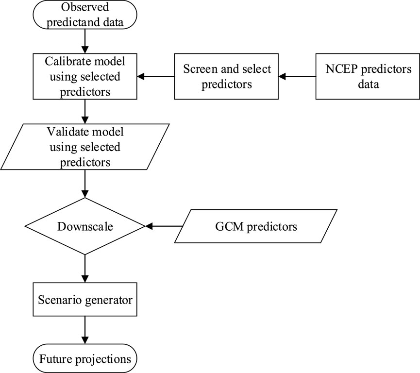
FIGURE 2. Methodology adopted by SDSM for downscaling and scenario generation.

The pivotal step in statistical downscaling is identifying the effective predictors, which is known as ‘screening of predictors’. In this study, the correlation coefficient, R, between predictors and predictand, was determined outside the SDSM to bring the values to an acceptable limit (Hashmi et al., 2011). The value of R has been calculated according to Equation 8:

$\mathrm{R}=\frac{\sum \left({\mathrm{x}}_{\mathrm{i}}-\overline{\mathrm{x}}\right)\left({\mathrm{y}}_{\mathrm{i}}-\overline{\mathrm{y}}\right)}{\sqrt{\sum {\left({\mathrm{x}}_{\mathrm{i}}-\overline{\mathrm{x}}\right)}^2\sum {\left({\mathrm{y}}_{\mathrm{i}}-\overline{\mathrm{y}}\right)}^2}}(8)$

where R is the correlation coefficient, x_i is a value of the x variable in the sample, $\overline{\mathrm{x}}$ is the mean of the x values, y_i is a value of the y variable in the sample, and $\overline{y}$ is the mean of the y values.

Predictor screening for temperature was straightforward, but for precipitation, certain values of SDSM parameters such as “variance inflation” and “event threshold” were tried. Simultaneously, sets of predictors were kept changing until the maximum coefficient of determination between monthly observed and simulated data was obtained (Hashmi et al., 2011). The mathematical equation for R² is given as Equation 9:

${\mathrm{R}}^2=\frac{{\left(\sum \left[{\mathrm{X}}_{\mathrm{i}}-{\mathrm{X}}_{\mathrm{a}\mathrm{v}}\right]\left[{\mathrm{Y}}_{\mathrm{i}}-{\mathrm{Y}}_{\mathrm{a}\mathrm{v}}\right]\right)}^2}{{\sum \left({\mathrm{X}}_{\mathrm{i}}-{\mathrm{X}}_{\mathrm{a}\mathrm{v}}\right)}^2{\sum \left({\mathrm{Y}}_{\mathrm{i}}-{\mathrm{Y}}_{\mathrm{a}\mathrm{v}}\right)}^2}(9)$

where X_i is a measured value, X_av is the mean of the measured values, Y_i is a simulated value, and Y_av is the mean of the simulated values. Data were divided into two parts: 1989 to 2000 was used for calibration while 2001 to 2005 was used for model validation. The stochastic weather generator was employed to produce 20 ensembles of weather series and the mean of those ensembles was compared with time series of the confirmation period. The calibrated model was then used for projection of temperature and precipitation over the selected period (2041–2060). The variation in precipitation and temperature was acquired from the percent change/absolute difference of the projected predictand with respect to the monthly mean of the observed period.

4 Results and discussion

4.1 Observed data

Table 2 shows a mixed result of nonsignificant increasing and decreasing trends in annual maximum temperature and precipitation. Among the nonsignificant temperature trends, all the stations showed decreasing levels (with Dir being the highest and Kalam the lowest) except for Saidu Sharif. This agrees with the study of Chaudhry et al., 2009, which reported that the northwestern part of the country had negative temperature trends, similar to the conclusions of Srinivas and Kumar (2006) who observed temperatures decreasing to −26°C in the northern hilly regions of the country. This is also in agreement with Anjum et al. (2019) who found no significant decreasing or increasing temperature trends in any of the zones of Swat.

TABLE 2

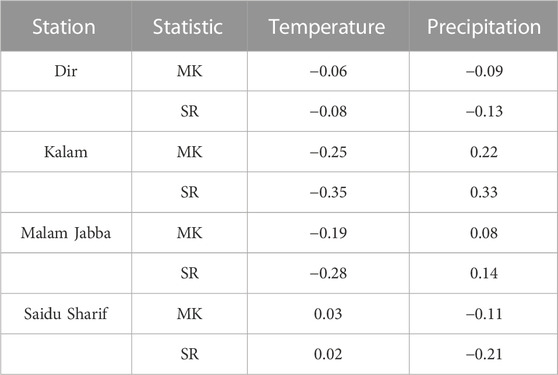
TABLE 2. Results of Man-Kendall and Spearman’s rho tests at 5% significance level.

Similar to the findings with regard to temperature, precipitation showed mixed results of nonsignificant decreasing and increasing trends. Two stations Dir and Saidu Sharif (with Dir being higher) showed a nonsignificant decreasing trend while Kalam and Malam Jabba (Kalam being higher) revealed a nonsignificant increasing trend. Similar results were revealed by the study of Ali and Iqbal (2012) that concluded there was no obvious trend in annual maximum rainfall at different stations of K.P including D.I. Khan, Peshawar, Parachinar, and Dir. This was further supported by Chaudhry et al. (2009) who stated that the precipitation trend was highly variable in spatio-temporal terms across Pakistan. Research conducted by Ahmad et al. (2014) showed that for annual precipitation, no significant trends were noted in the entire Swat River Basin which supported the findings of the current study. Similar conclusions were reached in the study of Ahmad et al. (2018) who claimed that annual precipitation exhibited an increasing trend at four stations in the northeastern region and a decreasing trend at two stations in the southeastern parts of the Upper Indus Basin. This also matched with (Khattak et al., 2011) where there were indefinite patterns of precipitation in the Upper Indus Basin. These changes in precipitation could cause Pakistan to suffer disasters like floods and droughts in the near future. Changing precipitation trends can be attributed to increasing aerosols from anthropogenic activities, deforestation, decreasing global monsoon circulation, global climate shifts, and changes in land use practices (Ahmad et al., 2014).

4.2 Projection of temperature and precipitation

4.2.1 Screening of predictors

This step is supposed to identify suitable sets of predictors from NCEP/NCAR reanalysis datasets based on maximum correlation. Selection of predictors varies depending on geography of the area and the characteristics of the predictand (Anandhi et al., 2009). Details of all NCEP predictors are given in Table 3 (Al-Mukhtar and Qasim, 2019). The ones in bold text were chosen for calibration of temperature, those in bold, erect text for calibration of precipitation, while bold, erect, and underlined text (nceps500-gl) was used in calibration of both temperature and precipitation. These sets of predictors were obtained through the use of maximum correlation coefficients and coefficients of determination between observed and simulated data. The shortlisted predictors for areal and station temperature included ncepp1-fgl, ncepp500-gl, ncepshumgl, nceps500-gl, nceps850-gl, and nceptempgl. The temperature predictors selected in this study were the same (excluding the first two) as in (Al-Mukhtar and Qasim, 2019), where the differences in two predictors could be ascribed to the difference between terrain and climate of the two areas. The relationship between these predictors is rational because they are correlated with the variation in temperature properties by thermal advection (Al-Mukhtar and Qasim, 2019).

TABLE 3

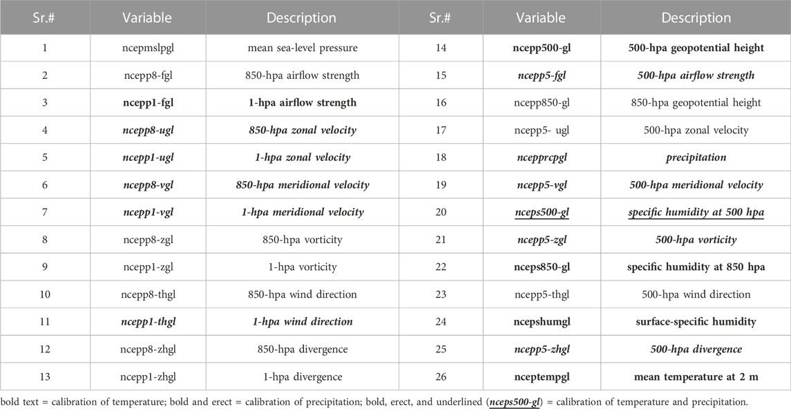
TABLE 3. Description of all NCEP variables (those in bold were chosen for model calibration).

The coefficient of determination between NCEP predictors and precipitation at individual stations was not favorable, so areal precipitation (the average of daily precipitation of all stations) was used; a similar approach was adopted by (Hashmi et al., 2011). Shortlisted predictors for areal precipitation included ncepp1-ugl, ncepp1-vgl, ncepp1-thgl, ncepp5-fgl, ncepp5-vgl, ncepp5-zgl, ncepp5-zhgl, ncepp8-ugl, ncepp8-vgl, ncepprcpgl, and nceps500-gl. Hessami et al. (2008) claimed that these parameters were linked with precipitation as their synchronous variation relied on the saturation phase of water vapor in the earth’s atmosphere.

4.2.2 Calibration and validation

The model having the maximum coefficient of determination and somewhat similar standard deviations between observed and simulated time series was considered as successfully calibrated and validated (Hashmi et al., 2011). Figure 3 shows comparisons between observed and simulated precipitation (areal) and the standard deviation. It is obvious that there is negligible variation between the observed and simulated standard deviations except in December for which the model slightly overestimated the observed precipitation. Similar results were found between observed and simulated temperatures (areal and station-wise).

FIGURE 3

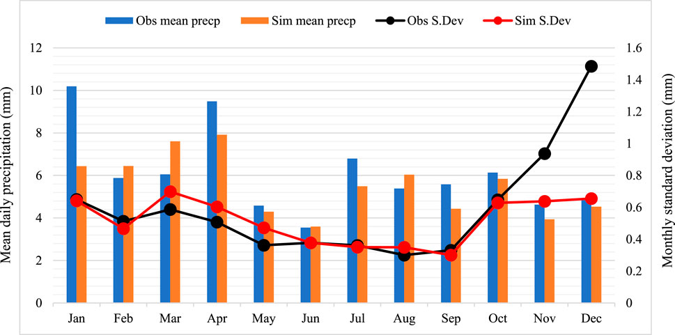
FIGURE 3. SDSM calibration of observed and simulated areal precipitation characteristics.

Figure 4 indicates that during the validation period, the SDSM overestimated the simulated precipitation for the months of February and October because of the extreme precipitation events in those months. Downscaling models are mostly assumed to be less capable of modeling the variance and standard deviation of the historical precipitation data with significant accuracy (Wilby et al., 2004; Hashmi et al., 2011). These models are often calibrated in ways not specifically intended for handling extreme events about which limited information is available (Wilby et al., 2004). Model calibration and validation of areal temperature as well as individual stations were performed in the same way and quite similar results were produced. Calibration and confirmation of the model was also verified in terms of the R² value between the monthly observed and simulated data (Table 4).

FIGURE 4

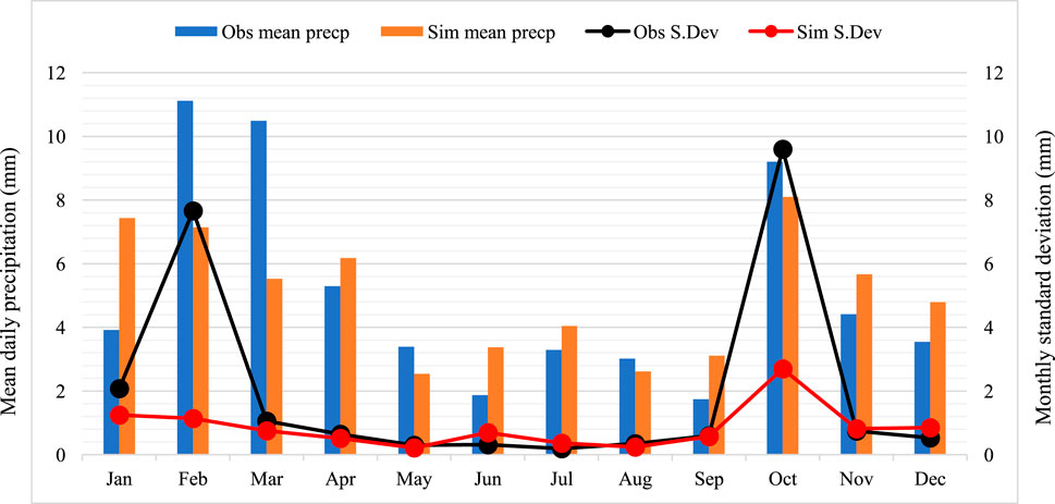
FIGURE 4. SDSM validation of observed and simulated areal precipitation characteristics.

TABLE 4

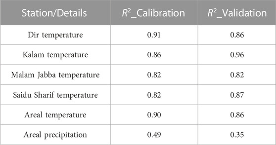
TABLE 4. Details of monthly coefficient of determination for calibration/validation periods.

4.2.3 Downscaling future climate scenarios

Based on RCP scenarios generated from CanESM2 GCM, the SDSM was run for projection of precipitation and temperature for the period 2041 to 2060. Figure 5 shows the change in projected temperature compared to the observed temperature and a significant change was noted for Dir, a 2.8°C rise under RCP 2.6, a 2.5°C increase under RCP 4.5, and a 2.98°C increase against RCP 8.5. The minimum increase in future temperatures has been observed at Saidu Sharif: 0.61°C, 0.35°C and 0.77°C under RCP 2.6, 4.5 and 8.5, respectively. The temperatures at Kalam (RCP 2.6_ 1.03°C RCP 4.5_0.69°C, RCP 8.5_1.37°C) and Malam Jabba (RCP 2.6_ 0.77°C, RCP 4.5_0.67°C, RCP 8.5_1.22°C) showed minimal differences between them. The minimum increase in temperature of all stations was noted with RCP 4.5, while the maximum increase occurred under RCP 8.5. Similar to the Dir station, the areal temperature also showed a remarkable increase in projected temperature of 2.2°C, 2.3°C, and 2.5°C under RCP 2.6, 4.5, and 8.5, respectively. Unlike station temperatures, the minimum temperature was observed by RCP 2.6, then 4.5 and finally by RCP 8.5. This is consistent with the study of Maida and Ghulam (2011) that determined the frequency of extreme precipitation and temperature in Pakistan, and found that the magnitude of the minimum and maximum temperatures was increasing, especially in Balochistan, Punjab, Azad Kashmir, and northern areas.

FIGURE 5

FIGURE 5. Changes in projected annual maximum temperatures.

The seasonal variation in temperatures was also quite alarming. Figure 6 shows that for areal temperatures in spring, summer, and autumn, there has been a rise almost exceeding 2°C under all RCPs except RCP 4.5, which experienced an increase of 1.3°C in summer. Furthermore, winter temperatures have exhibited a surge of 1.9°C, 1.8°C, and 2.7°C under RCP 2.6, 4.5, and 8.5, respectively. Dir is the only station that had an increasing trend in seasonal temperatures under all RCPs (Figure 7A). Under RCP 4.5, all seasons showed increases >2°C. RCP 2.6 revealed a rise of 2.2°C, 2.7°C, 4.1°C, and 3.2°C in winter, spring, summer and autumn, respectively. It is evident from Figure 7B that Kalam station experienced a remarkable increase in winter and autumn temperatures under all RCPs. RCP 4.5 in the summer season showed a decrease of 1.6°C, while RCP 2.6 and 8.5 of spring experienced a rise of 1.4°C and 1.2°C, respectively. Temperatures at Malam Jabba and Saidu Sharif exhibited significant increases in winter and notable declines in summer (Figure 7C, D).

FIGURE 6

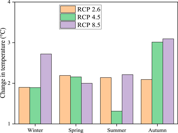
FIGURE 6. Changes in seasonal maximum areal temperatures.

FIGURE 7

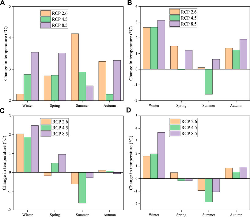
FIGURE 7. Changes in maximum seasonal temperatures of Dir (A), Kalam (B), Malam Jabba (C), and Saidu Sharif (D).

Figure 8 shows percent changes in the annual and seasonal maximum precipitation time series by the middle of this century and the variation in precipitation was 12% for RCP 2.6 and 4.5, and 11% for RCP 8.5. This is compatible with the study of Hartmann and Buchanan (2014) who found increasing trends in extreme precipitation indices in the Indus Basin. The same was acknowledged by Rahman et al. (2018) who studied the spatio-temporal changes in rainfall and drought in Khyber Pakhtunkhwa, and all stations revealed positive skewness excluding Balakot while the major change was found at the Parachinar and Balakot stations. On a seasonal scale, the greatest increase in maximum precipitation was observed in summer (RCP 2.6_11%, RCP 4.5_20%, RCP 8.5_12%) and autumn (RCP 2.6_11%, RCP 4.5_32%, RCP 8.5_14%), while the rise in maximum precipitation in winter (RCP 2.6_11%, RCP 4.5_6%, RCP 8.5_6%), and spring (RCP 2.6_15%, RCP 4.5_1%, RCP 8.5_9%), was minor compared to autumn and summer. This agrees with the results of Archer and Fowler (2004) who investigated the spatio-temporal changes in precipitation in the Upper Indus Basin, and a remarkable increase in summer, winter and annual precipitation at certain stations was observed. This is also supported by the study of Hussain and Lee (2013) who analyzed the regional/seasonal changes in precipitation extremes in Pakistan and found that in all seasons, a rising trend in extreme precipitation occurred in the northeastern part, while a decreased tendency prevailed in the southwestern portion of the country.

FIGURE 8

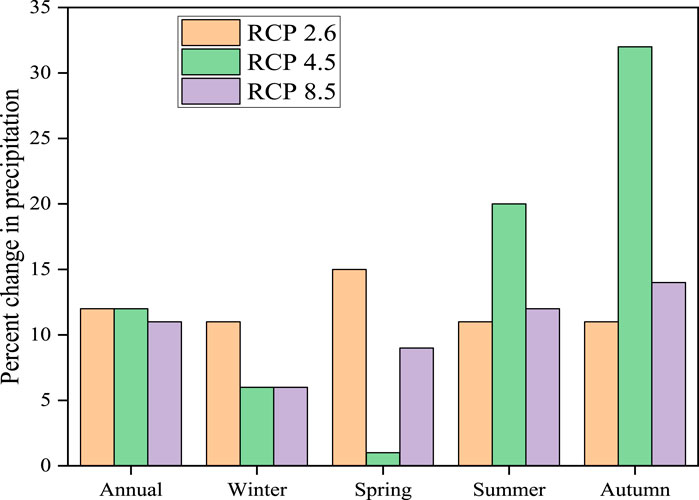
FIGURE 8. Changes in projected annual and seasonal maximum precipitation.

Figure 9 shows that the maximum wet spell length has increased annually by12%, 11%, and 34% under RCP 2.6, 4.5, and 8.5, respectively, and on a seasonal scale except for winter, where a decrease of 3%, 8%, and 1% occurred for RCP 2.6, 4.5, and 8.5, respectively. A greater than 12% increase in the maximum wet spell in spring was seen for all RCPs, while the summer season had an increase of 15%, 7%, and 20% under RCP 2.6, 4.5, and 8.5, respectively. Because winter had a downward trend in maximum wet spell, an upward trend in the dry spell occurred in the same season (Figure 10). Similarly, the spring and autumn seasons revealed a decreasing trend in the length of the dry spell and an upward trend in the wet spell in the same seasons. Similar results were presented by Salma et al. (2012) who studied rainfall variation in different climate zones of the country, and their results showed a declining trend of −1.18 mm/decade around the country.

FIGURE 9

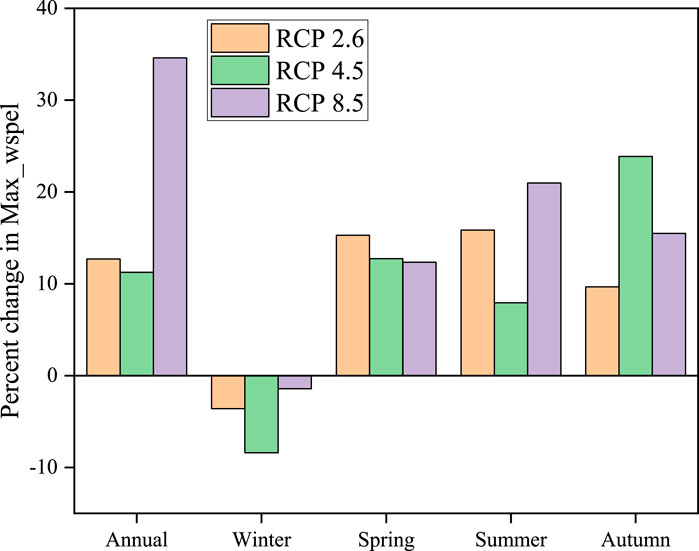
FIGURE 9. Percent change in maximum wet spell length.

FIGURE 10

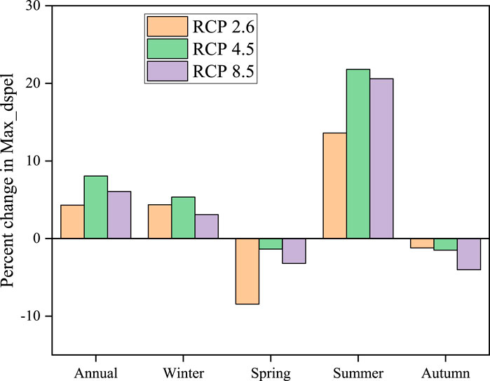
FIGURE 10. Percent change in maximum dry spell length.

Prolonged periods with high or low temperature, extensive or no rainfall may cause stress on flora, fauna and humans. These periods have other hydrological and ecological consequences. They can influence growth and yield of plants and crops, production of milk in animals, conception in cows, reproduction of dairy bulls, and modifications in the growing seasons of crops, with serious effects on the water cycle and damage to the economy of a region (Anandhi et al., 2016).

5 Conclusion

This study aimed to investigate the variations in maxima of temperature and precipitation in the Swat River Basin using observed data from four weather stations to evaluate the vulnerability of the watershed to climate change. The SDSM, which is a popular statistical downscaling tool, was used to generate local scale future climate data of four selected stations in the study watershed based on the outputs of selected GCM (CanESM2) under three representative concentration pathways: RCP 2.6, 4.5, and 8.5. Screening for the most suitable predictors for SDSM calibration in precipitation simulation was the major challenge of this study due to the complex topography of the basin and the stochastic nature of precipitation.

Data from four available climate observation stations in the basin were analyzed in terms of seasonal and annual maxima to determine current and future trends of climate extremes. A mixed result of nonsignificant increasing and decreasing trends in annual maximum temperatures and precipitation was found in the observed data (all stations showed decreasing temperature trends except Saidu Sharif). For precipitation, the northwestern areas showed nonsignificant decreasing trends while the northeastern regions revealed increasing trends. The projected maximum temperature (annual and seasonal) showed a rising trend while the maximum precipitation revealed increasing trends on an annual and seasonal time series, particularly in summer and autumn. On the whole, the results revealed that increases in maximum temperature lead to increased numbers of dry days and extreme precipitation events.

Data were scarce in the study area because of the few and unevenly distributed meteorological stations; still, the results are important for current as well as future economic development of the country in terms of agriculture, tourism and hydropower. The outcomes of our study will help researchers to appreciate the sensitivity of the Swat River Basin to extreme climatic events and will serve as a source for evaluating the impact of climate change on environment, agriculture, human health, tourism, and water resources in the area, and for strengthening local decision-making, adaptive capacity, and strategic planning.

Data availability statement

The original contributions presented in the study are included in the article/Supplementary Material. Further inquiries can be directed to the corresponding authors.

Author contributions

MH conceptualized and supervised the research, AJ contributed in data collection and designing methodology, and HI helped in model calibration and validation. The formal analysis and write up of the original draft was done by WA, data curation by SA, and SR reviewed and edited the manuscript.

Conflict of interest

HI was employed by the Rawalpindi Waste Management Company.

The remaining authors declare that the research was conducted in the absence of any commercial or financial relationships that could be construed as a potential conflict of interest.

Publisher’s note

All claims expressed in this article are solely those of the authors and do not necessarily represent those of their affiliated organizations, or those of the publisher, the editors and the reviewers. Any product that may be evaluated in this article, or claim that may be made by its manufacturer, is not guaranteed or endorsed by the publisher.

References

Ahmad, I., Tang, D., Wang, T., Wang, M., and Wagan, B. (2014). Precipitation trends over time using mann-kendall and spearman’s rho tests in Swat River Basin, Pakistan. Adv. Meteorology 2015, 1–15. Article ID 431860. doi:10.1155/2015/431860

CrossRef Full Text | Google Scholar

Ahmad, I., Zhang, F., Tayyab, M., Anjum, M. N., Zaman, M., Liug, J., et al. (2018). Spatiotemporal analysis of precipitation variability in annual, seasonal and extreme values over upper Indus River basin. Atmos. Res. 213, 346–360. doi:10.1016/j.atmosres.2018.06.019

CrossRef Full Text | Google Scholar

Al-Mukhtar, M., and Qasim, M. (2019). Future predictions of precipitation and temperature in Iraq using the statistical downscaling model. Arab. J. Geosci. 12 (2), 25. doi:10.1007/s12517-018-4187-x

CrossRef Full Text | Google Scholar

Alexander, M. A., Scott, J. D., Mahoney, K., and Barsugli, J. (2013). Greenhouse gas induced changes in summer precipitation over Colorado in NARCCAP regional climate models. J. Clim. 26, 8690–8697. doi:10.1175/jcli-d-13-00088.1

CrossRef Full Text | Google Scholar

Ali, M., and Iqbal, M. (2012). A probabilistic approach for estimating return periods of extreme annual rainfall in different cities of Khyber Pakhtunkhwa (KPK), Pakistan. Nucl. 49 (2), 107–114.

Google Scholar

Amell, N. W. (2003). Relative effects of multi-decadal climatic variability and changes in the mean and variability of climate due to global warming: Future streamflows in britain. J. Hydrol. X. 270, 195–213. doi:10.1016/s0022-1694(02)00288-3

CrossRef Full Text | Google Scholar

Anandhi, A., Hutchinson, S., Harrington, J., Rahmani, V., Kirkham, M. B., and Rice, C. W. (2016). Changes in spatial and temporal trends in wet, dry, warm and cold spell length or duration indices in Kansas, USA. Int. J. Climatol. 36 (12), 4085–4101. doi:10.1002/joc.4619

CrossRef Full Text | Google Scholar

Anandhi, A., Shrinivas, V. V., Nanjundiah, R. S., and Kumar, D. N. (2009). Role of predictors in downscaling surface temperature to river basin in India for IPCC SRES scenarios using support vector machine. Int. J. Climatol. 29 (4), 583–603. doi:10.1002/joc.1719

CrossRef Full Text | Google Scholar

Anderegg, W. R. L., Prall, J. W., Harold, J., and Schneider, S. H. (2010). Expert credibility in climate change. Proc. Natl. Acad. Sci. U. S. A. 107, 12107–12109. doi:10.1073/pnas.1003187107

PubMed Abstract | CrossRef Full Text | Google Scholar

Anjum, M. N., Ding, Y., Shangguan, D., Ijaz, M. W., and Zhang, S. (2016). Evaluation of high resolution satellite-based real-time and post-real-time precipitation estimates during 2010 extreme flood event in Swat River Basin, Hindukush Region. Adv. Meteorology 2016, 1–8. doi:10.1155/2016/2604980

CrossRef Full Text | Google Scholar

Anjum, M. N., Ding, Y., Shangguan, D., Liu, J., Ahmad, I., Ijaz, M. W., et al. (2019). Quantification of spatial temporal variability of snow cover and hydro-climatic variables based on multi-source remote sensing data in the Swat watershed, Hindukush Mountains, Pakistan. Meteorol. Atmos. Phys. 131 (3), 467–486. doi:10.1007/s00703-018-0584-7

CrossRef Full Text | Google Scholar

Archer, D. R., and Fowler, H. J. (2004). Spatial and temporal variations in precipitation in the Upper Indus Basin, global teleconnections and hydrological implications. Hydrol. Earth Syst. Sci. 8, 47–61. doi:10.5194/hess-8-47-2004

CrossRef Full Text | Google Scholar

Bahadar, I., Shafique, M., Khan, T., Tabassum, I., and Ali, M. Z. (2015). Flood hazard assessment using hydro dynamic model and GIS/RS tools: A case study of babuzai kabal tehsil swat basin. J. Himal. Earth Sci. 48 (2), 29–138.

Google Scholar

Chaudhry, Q. U. Z., Mahmood, A., Rasul, G., and Afzaal, M. (2009). Climate change indicators of Pakistan. Technical Report No. PMD 22/2009. Islamabad: Pakistan Meteorological Department, 1–43.

Google Scholar

Chu, J. T., Xia, J., Xu, C. Y., and Singh, V. P. (2010). Statistical downscaling of daily mean temperature, pan evaporation and precipitation for climate change scenarios in Haihe River, China. Theor. Appl. Climatol. 99, 149–161. doi:10.1007/s00704-009-0129-6

CrossRef Full Text | Google Scholar

Dong, Z., Liu, H., Baiyinbaoligao, H., Hu, H., Khan, M. Y. A., Wen, J., et al. (2022). Future projection of seasonal drought characteristics using CMIP6 in the Lancang-Mekong River Basin. J. Hydrology 610, 127815. doi:10.1016/j.jhydrol.2022.127815

CrossRef Full Text | Google Scholar

Fang, J., Kong, F., Fang, J., and Zhao, L. (2018). Observed changes in hydrological extremes and flood disaster in yangtze River Basin: Spatial–temporal variability and climate change impacts. Nat. Hazards (Dordr). 93, 89–107. doi:10.1007/s11069-018-3290-3

CrossRef Full Text | Google Scholar

Gajbhiye, S., Meshram, C., Singh, S. K., Srivastava, P. K., and Islam, T. (2016). Precipitation trend analysis of Sindh River basin, India, from 102-year record (1901-2002). Atmos. Sci. Lett. 17, 71–77. doi:10.1002/asl.602

CrossRef Full Text | Google Scholar

Hartmann, H., and Buchanan, H. (2014). Trends in extreme precipitation events in the Indus River Basin and flooding in Pakistan. Atmosphere-Ocean 52 (1), 77–91. doi:10.1080/07055900.2013.859124

CrossRef Full Text | Google Scholar

Hashmi, M. Z., Shamseldin, A. Y., and Melville, B. W. (2011). Comparison of SDSM and LARS- WG for simulation and downscaling of extreme precipitation events in a watershed. Stoch. Environ. Res. Risk Assess. 25, 475–484. doi:10.1007/s00477-010-0416-x

CrossRef Full Text | Google Scholar

Hessami, M., Gachon, P., Ouarda, T. B. M. J., and St-Hilaire, A. (2008). Automated regression based statistical downscaling tool. Environ. Model. Softw. 23 (6), 813–834. doi:10.1016/j.envsoft.2007.10.004

CrossRef Full Text | Google Scholar

Huang, J., Zhang, J., Zhang, Z., Xu, C., Wang, B., and Yao, J. (2011). Estimation of future precipitation change in the Yangtze River basin by using statistical downscaling method. Stoch. Environ. Res. Risk Assess. 25 (6), 781–792. doi:10.1007/s00477-010-0441-9

CrossRef Full Text | Google Scholar

Hussain, M. S., and Lee, S. (2013). The regional and the seasonal variability of extreme precipitation trends in Pakistan. Asia. Pac. J. Atmos. Sci. 49 (4), 421–441. doi:10.1007/s13143-013-0039-5

CrossRef Full Text | Google Scholar

Ikram, F., Afzaal, M., Bukhari, S. A. A., and Ahmed, B. (2016). Past and future trends in frequency of heavy rainfall events over Pakistan. Pak J. Met. 12, 57–78.

Google Scholar

IPCC (2013). Contribution of working group i to the fifth assessment report of the intergovernmental panel on climate change. Cambridge, United Kingdom and New York, USA: Cambridge University Press, 1535.

Google Scholar

IPCC First assessment report (1990). Climate change: The IPCC scientific assessment. Cambridge: Cambridge University Press.

Google Scholar

IPCC (2007). Summary for policymakers. Contribution of working group I to the fourth assessment report of the intergovernmental panel on climate change. Cambridge, United Kingdom: Cambridge University Press.

Google Scholar

Khadka, D., and Pathak, D. (2016). Climate change projection for the marsyangdi river basin, Nepal using statistical downscaling of GCM and its implications in geodisasters. Geoenvironmental Disasters 3 (1), 15. doi:10.1186/s40677-016-0050-0

CrossRef Full Text | Google Scholar

Khan, S., and Hasan, M. (2016). Climate change impacts and adaptation to flow of Swat River and glaciers in hindu kush ranges, swat district, Pakistan (2003-2013). Int. J. Econ. Environ. Geol. 7 (1), 24–35.

Google Scholar

Khattak, M. S., Babel, M. S., and Sharif, M. (2011). Hydro-meteorological trends in the upper Indus River basin in Pakistan. Clim. Res. 46, 103–119. doi:10.3354/cr00957

CrossRef Full Text | Google Scholar

Lehmann, E. L. (1975). Nonparametrics, statistical methods based on ranks. San Francisco, Calif, USA: Holden Day.

Google Scholar

Li, K., Tian, F., Khan, M. Y. A., Xu, R., He, Z., Yang, L., et al. (2021). A high-accuracy rainfall dataset by merging multiple satellites and dense gauges over the southern Tibetan Plateau for 2014–2019 warm seasons. Earth Syst. Sci. Data 13, 5455–5467. doi:10.5194/essd-13-5455-2021

CrossRef Full Text | Google Scholar

Maida, Z., and Ghulam, R. (2011). Frequency of extreme temperature and precipitation events in Pakistan 1965-2009. Sci. Int. (Lahore) 23 (4), 313–319.

Google Scholar

Malik, M. I., and Ahmad, F. (2014). Flood inundation mapping and risk zoning of the Swat River Pakistan using HEC-RAS model. J. Sci. Technol. l3, 45–52.

Google Scholar

Owolabi, S. T., Madi, K., and Kalumba, A. M. (2020). Comparative evaluation of spatio-temporal attributes of precipitation and streamflow in buffalo and tyume catchments, eastern cape, south Africa. Environ. Dev. Sustain. 23, 4236–4251. doi:10.1007/s10668-020-00769-z

CrossRef Full Text | Google Scholar

Pal, I., and Al-Tabbaa, A. (2011). Assessing seasonal precipitation trends in India using parametric and non-parametric statistical techniques. Theor. Appl. Climatol. 103, 1–11. doi:10.1007/s00704-010-0277-8

CrossRef Full Text | Google Scholar

Rahman, A. U., and Khan, A. N. (2011). Analysis of flood causes and associated socio economic damages in the Hindukush region. Nat. Hazards (Dordr). 59 (3), 1239–1260. doi:10.1007/s11069-011-9830-8

CrossRef Full Text | Google Scholar

Rahman, G., Rahman, A., Samiullah, , and Dawood, M. (2018). Spatial and temporal variation of rainfall and drought in Khyber Pakhtunkhwa Province of Pakistan during 1971-2015. Arab. J. Geosci. 11, 46. doi:10.1007/s12517-018-3396-7

CrossRef Full Text | Google Scholar

Reiter, A., Weidinger, R., and Mauser, W. (2012). Recent Climate Change at the Upper Danube A temporal and spatial analysis of temperature and precipitation time series. Clim. Change 111, 665–696. doi:10.1007/s10584-011-0173-y

CrossRef Full Text | Google Scholar

Sabir, M. A., Rehman, S. S., Umar, M., Waseem, A., Farooq, M., Fariduulah, , et al. (2014). Assessment of hydro power potential of swat, kohistan himalayas: A solution for energy shortfall in region. Water Resour. 41 (5), 612–618. doi:10.1134/s0097807814050091

CrossRef Full Text | Google Scholar

Saddique, N., Khaliq, A., and Bernhofer, C. (2020). Trends in temperature and precipitation extremes in historical (1961–1990) and projected (2061–2090) periods in a data scarce mountain basin, northern Pakistan. Stoch. Environ. Res. Risk Assess. 34, 1441–1455. doi:10.1007/s00477-020-01829-6

CrossRef Full Text | Google Scholar

Salma, S., Rehman, S., and Shah, M. (2012). Rainfall trends in different climate zones of Pakistan. Pak J. Met. 9 (17).

Google Scholar

Scanlon, B. R., Jolly, I., Sophocleous, M., and Zhang, L. (2007). Global impacts of conversions from natural to agricultural ecosystems on water resources: Quantity versus quality. Water Resour. Res. 43, W03437. doi:10.1029/2006WR005486

CrossRef Full Text | Google Scholar

Sen, P. K. (1968). Estimates of the regression coefficient based on Kendall’s tau. J. Am. Stat. Assoc. 63 (324), 1379–1389. doi:10.1080/01621459.1968.10480934

CrossRef Full Text | Google Scholar

Sneyers, R. (1990). On the statistical analysis of series of observations. Technical Note 143, WMO no. 415. Geneva, Switzerland: World Meteorological Organization.

Google Scholar

Srinivas, K., and Kumar, P. K. D. (2006). Atmospheric forcing on the seasonal variability of sea level at Cochin, southwest coast of India. Cont. Shelf Res. 26, 1113–1133. doi:10.1016/j.csr.2006.03.010

CrossRef Full Text | Google Scholar

Sultan-i-Rome (2005). Forestry in the princely state of swat and Kalam (north-west Pakistan): A historical perspective on norms and practices. IP6 Working Paper No. 6. North-south Dialogue: Swiss National Centre of Competence in Research, 126.

Google Scholar

Trenberth, K. E. (2011). Changes in precipitation with climate change. Clim. Res. 47, 123–138. doi:10.3354/cr00953

CrossRef Full Text | Google Scholar

Wilby, R. L., Dawson, C. W., and Barrow, E. M. (2002). SDSM-a decision support tool for the assessment of regional climate change impacts. Environ. Model. Softw. 17, 145–157. doi:10.1016/s1364-8152(01)00060-3

CrossRef Full Text | Google Scholar

Wilby, R. L., Charles, S. P., Zorita, E., Timbal, B., Whetton, P., and Mearns, L. O. (2004). Guidelines for use of climate scenarios developed from statistical downscaling methods. Supporting material of the Intergovernmental Panel on Climate Change, 27. Available from the DDC of IPCC TGCIA.

Google Scholar

Wilby, R. L., Hay, L. E., and Leavesley, G. H. (1999). A comparison of downscaled and raw GCM output: Implications for climate change scenarios in the san juan River basin, Colorado. J. Hydrol. X. 225, 67–91. doi:10.1016/s0022-1694(99)00136-5

CrossRef Full Text | Google Scholar

Wu, P., Christidis, N., and Stott, P. (2013). Anthropogenic impact on Earth's hydrological cycle. Nat. Clim. Chang. 3, 807–810. doi:10.1038/nclimate1932

CrossRef Full Text | Google Scholar

Xu, C. Y., Gong, L., Jiang, T., Chen, D., and Singh, V. P. (2006). Analysis of spatial distribution and temporal trend of reference evapotranspiration and pan evaporation in Changjiang (Yangtze River) catchment. J. Hydrol. X. 327, 81–93. doi:10.1016/j.jhydrol.2005.11.029

CrossRef Full Text | Google Scholar

Xu, R., Hu, H., Tian, F., Li, C., and Khan, M. Y. A. (2019). Projected climate change impacts on future streamflow of the Yarlung Tsangpo Brahmaputra River. Glob. Planet. Change 175, 144–159. doi:10.1016/j.gloplacha.2019.01.012

CrossRef Full Text | Google Scholar

Yue, S., Pilon, P., Phinney, B., and Cavadias, G. (2002). The influence of autocorrelation on the ability to detect trend in hydrological series. Hydrol. Process. 16, 1807–1829. doi:10.1002/hyp.1095

CrossRef Full Text | Google Scholar

Zhang, Q., Xu, C.-Y., Tao, H., Jiang, T., and Chen, Y. D. (2010). Climate changes and their impacts on water resources in the arid regions: A case study of the tarim River basin, China. Stoch. Environ. Res. Risk Assess. 24, 349–358. doi:10.1007/s00477-009-0324-0

CrossRef Full Text | Google Scholar