Airborne small-footprint full-waveform LiDAR data for urban land cover classification

Airborne small-footprint full-waveform LiDAR data have a unique ability to characterize the landscape because it contains rich horizontal and vertical information. However, a few studies have fully explored its role in distinguishing different objects in the urban area. In this study, we examined the efficacy of small-footprint full-waveform LiDAR data on urban land cover classification. The study area is located in a suburban area in Beijing, China. Eight land cover classes were included: impervious ground, bare soil, grass, crop, tree, low building, high building, and water. We first decomposed waveform LiDAR data, from which a set of features were extracted. These features were related to amplitude, echo width, mixed ratio, height, symmetry, and vertical distribution. Then, we used a random forest classifier to evaluate the importance of these features and conduct the urban land cover classification. Finally, we assessed the classification accuracy based on a confusion matrix. Results showed that A_first was the most important feature for urban land cover classification, and the other seven features, namely, ω_first, H_Eavg, nH_Eavg, R_Aω, SYM_S, S_rise, and ωR_{f_fl}, also played important roles in classification. The random forest classifier yielded an overall classification accuracy of 94.7%, which was higher than those from previous LiDAR-derived classifications. The results indicated that full-waveform LiDAR data could be used for high-precision urban land cover classification, and the proposed features could help improve the classification accuracy.

1 Introduction

Urban areas are usually made up of many types of natural and artificial surfaces (Myint et al., 2011; Chen et al., 2018). Urban land cover products play an important role in urban planning, monitoring, and managing (Zhou, 2013; Man et al., 2015). However, the urban landscape is complex and rapidly changing, which makes urban mapping challenging (Chen et al., 2018). Remote sensing can acquire land cover information over large areas rapidly, and it has been widely used for land cover classification (Man et al., 2015; Gómez et al., 2016). High-resolution passive remote sensing data have rich spectral and textural information, which have been used to extract various object features to generate land cover maps (Dash et al., 2007; Zhou et al., 2009; Hansen et al., 2010; Jia et al., 2014; Wu et al., 2016). However, the problem of between-class spectral confusion, within-class spectral variation, the shadows in passive remote sensing imagery, and the lack of vertical information always limit the accuracy of urban mapping.

LiDAR is an active remote sensing technique, which can acquire both the horizontal and vertical information of objects, and has been used in many applications, such as digital terrain model generation, building modeling, and forest monitoring (Webster, 2006; Lee et al., 2009; Chen and Gao, 2014; Dong et al., 2017). In addition, LiDAR data have no shadow and can eliminate the displacement of the object, so it has a unique advantage in distinguishing different land cover types. In recent years, airborne LiDAR data have been utilized increasingly for land cover classification (Antonarakis et al., 2008; Sherba et al., 2014; Qin et al., 2015). However, discrete-return LiDAR data only contains three-dimensional point clouds with echo number and intensity information, which are insufficient for complex urban land cover classification (Mallet et al., 2011; Hellesen and Matikainen, 2013).

As the technology advance, full-waveform LiDAR with the ability to describe the complete reflected signal of each transmitted pulse has been introduced. Besides the distance measurement, more physical surface characteristics can be derived from the analysis of the reflection waveforms, thus providing great potential for complex urban land cover classification. Previous studies have studied urban land cover classification based on full-waveform LiDAR data (Guo et al., 2011; Chang et al., 2015). Mallet et al. (2011) extracted 19 geometrical features and 8 waveform features from full-waveform LiDAR data to classify urban region into building, ground, and vegetation, and their results showed that waveform features contributed most to the high classification accuracy (95.3%). Neuenschwander et al. (2009) extracted nine full-waveform features for land cover classification, and they found Gaussian amplitude was the most important feature, resulting in a classification accuracy of 85.8%. Zhou et al. (2015) extracted four waveform features to classify the targets as road, trees, buildings, and farmland, achieving a classification accuracy of 79.57%. Tseng et al. (2015) extracted waveform LiDAR features to classify five urban land cover types and obtained a classification accuracy of 86.01% (Tseng et al., 2015). However, these studies simply extracted waveform amplitude, echo width, and height features from full-waveform LiDAR data for urban land cover classification. They did not standardize the above features, nor did they consider the symmetry, vertical distribution, and shape of waveforms, resulting in insufficient classification types or low classification accuracy.

The main purpose of this research is to explore more possibilities of small-footprint full-waveform LiDAR data for urban land cover classification. For fulfilling this goal, this study identified four specific objectives:1) to preprocess the waveform LiDAR data and conduct a Gaussian decomposition; 2) to propose a series of new waveform features and extract them from the LiDAR data; 3) to evaluate the importance of variables and use a random forest classifier to classify urban land cover types; and 4) to evaluate the accuracy of urban land cover classification.

2 Study area and data

2.1 Study area

This study was carried out in a suburban area in Yanqing District, Beijing, China (115°57′13″E-115°58′40″E, 40°26′53″-40°28′37″), and the location of the study region is shown in Figure 1. The size of this study area is about 5.8 km². The land use of this area was dominated by residential land, mixed with a small amount of agricultural and commercial land. The land cover types in this study region are typical of urban and suburban environments, including high building (>3 layers), low building (1–3 layers), tree, grass, crop, impervious ground, bare soil, and water, in which the variety of the land cover makes it well suited for the goal of this study.

FIGURE 1

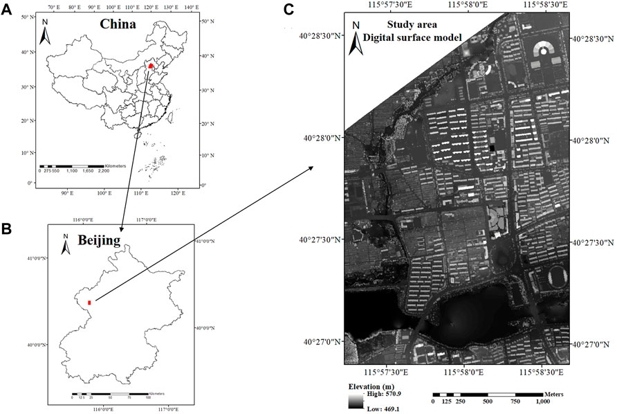
FIGURE 1. Location of the study region in Yanqing District, Beijing, China. (A) location of Beijing in China, (B) location of the study region in Beijing, (C) the study region.

2.2 LiDAR data

Airborne small-footprint full-waveform LiDAR data were obtained in July 2014 using a Leica ALS70-HA system. The wavelength of the laser pulse emitted by this system is 1,064 nm, and the pulse frequency is 50 kHz. In this survey, the system was operated with a beam divergence of 0.22 mrad at an average flying height of 1,600 m, so the footprint diameter was approximately 0.35 m. The flight lines were flown with a 50% side overlap, and the scanning angle was ±12°. The pulse density was about 8 echoes/m². The system was equipped with a high-precision global positioning system (GPS) and an inertial measurement unit (IMU), which could obtain the position and attitude information of the sensor. The horizontal accuracy of the LiDAR data was less than 10 cm, and the vertical accuracy was less than 15 cm.

2.3 Reference data

The reference samples of eight land cover types were randomly selected based on the LiDAR-derived digital surface model (DSM) and referring to the high-resolution Google Earth images. The geometric and orthophoto corrections have been carried out on the Google Earth images using LiDAR-derived DSM and digital terrain model (DTM). A total of 10,000 sampling points were selected for training the land cover classification model and assessing the classification accuracy. The rule for selecting a sampling point is to obtain the same object within a radius of 3 m around the sampling point (Luo et al., 2015). The number of the training and validation sampling points per class is shown in Table 1.

TABLE 1

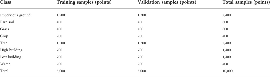
TABLE 1. The number of training and validation sampling points per class.

3 Methodology

The flowchart of the urban land cover classification procedure in this research is shown in Figure 2, which contains data preprocessing, waveform feature extraction, and land cover classification. We first preprocessed the full-waveform LiDAR data, including waveform denoising and smoothing. Then, we used a Gaussian decomposition algorithm to decompose the smoothed waveform LiDAR data into points and extracted a set of new waveform features. Finally, we classified these points into different land cover types using a random forest classifier.

FIGURE 2

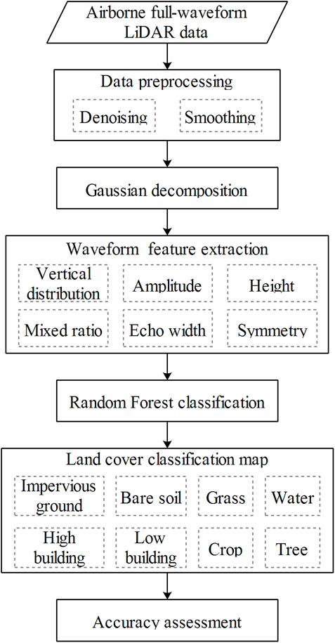
FIGURE 2. Flowchart of the land cover classification procedure in this study.

3.1 Waveform processing

3.1.1 Waveform preprocessing

Airborne small-footprint full-waveform LiDAR data should be preprocessed at first to make certain of the reliability of the extracted waveform features. Due to the system error, the limitations of sensor capacity, and the interactions between the emitted pulse and the ground object, there are some background noises in the original waveform LiDAR data. We should remove the background noises to obtain effective waveform signals. We used a frequency histogram method to calculate the average value of background noises from the original waveform data (Sun et al., 2008). Then, we subtracted them from the original waveform data to remove the background noises (Duong et al., 2008). After that, we used a Gaussian filter to smooth the waveform and thus obtained the smoothed waveform data (Mallet and Bretar, 2009).

3.1.2 Waveform decomposition

We performed the Gaussian decomposition on the preprocessed waveform data to obtain the point cloud data with waveform features. We first estimated the initial parameters of each Gaussian component of the waveform, including peak amplitude, peak position, and the standard deviation. Then, we used the Levenberg–Marquardt (LM) algorithm to optimize these Gaussian parameters. After waveform decomposition, each waveform was converted into several 3D points with a set of waveform features, including echo height, echo amplitude, echo width, and return number. The detailed process of the Gaussian decomposition of waveform data is shown in Wagner et al. (2006), and Figure 3 shows an example of the results of Gaussian decomposition.

FIGURE 3

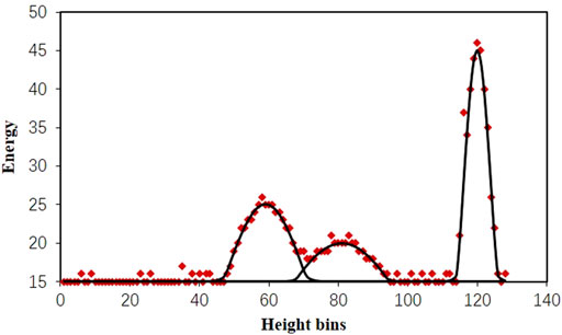
FIGURE 3. Representation of Gaussian decomposition: raw waveform (red points) and decomposed Gaussian components (black lines).

3.2 Feature extraction

Based on the decomposed waveform LiDAR data, we proposed and extracted 22 waveform features to represent the waveform data, which were related to amplitude, echo width, mixed ratio, height, symmetry, and vertical distribution.

Amplitude-related metrics:

• A_first: peak amplitude of the first echo of the waveform, which is derived from the Gaussian decomposition of the waveform.

• nA_first: normalized peak amplitude of the first echo, which is calculated as $n{A}_{first}=\frac{A_{first}}{A_{all}}$, where A_all is the sum of all echo amplitudes of the waveform.

• AR_{f_fl}: ratio of the first echo amplitude and the sum of the first and last echo amplitudes of the waveform. It can be calculated as $A{R}_{f\_fl}=\frac{A_{first}}{A_{first}+A_{last}}$, where A_last is the peak amplitude of the last echo of the waveform.

Echo-width-related metrics:

• ω_first: width of the first echo of the waveform, which is the standard deviation of the first Gaussian component, and it is derived from the Gaussian decomposition of the waveform.

• nω_first: normalized echo width of the first echo, which is calculated as $n{\omega }_{first}=\frac{{\omega }_{first}}{{\omega }_{all}}$, where ω_all is the sum of all echo widths of the waveform.

• ωR_{f_fl}: ratio of the first echo width and the sum of the first and last echo widths of the waveform. It can be calculated as $\omega R_{f\_fl}=\frac{{\omega }_{first}}{{\omega }_{first}+{\omega }_{last}}$, where ω_last is the echo width of the last echo of the waveform.

Mixed-ratio-related metrics:

• R_Aω: ratio of amplitude and width of the first echo of the waveform, and it is calculated as $R_{A\omega }=\frac{A_{first}}{{\omega }_{first}}$.

Height-related metrics:

• H_Eavg: energy weighted average height of the waveform. It is calculated as $H_{Eavg}={\displaystyle \sum }_{i=1}^N\frac{E_i}{E_{all}}\times H_i$, where E_i is the energy of bin i, E_all is the energy of all bins, H_i is the height of bin i, and N is the total number of bins of the waveform.

• nH_Eavg: ratio of the energy weighted average height and the height of the waveform. It is calculated as $n{H}_{Eavg}=\frac{H_{Eavg}}{H_w}$, where H_w is the height of the waveform.

• H_avg: average height of all bins of the waveform. It is calculated as $H_{avg}=\frac{{\displaystyle \sum }_{i=1}^N{H}_i}{N}$.

• nH_avg: ratio of the average height of all bins and the height of the waveform. It is calculated as $n{H}_{avg}=\frac{H_{avg}}{H_w}$.

Symmetry-related metrics:

• T_rise: the rise time of the first peak of the waveform, which is defined as the duration between the leading edge of the first echo and the first peak.

• T_fall: the fall time of the first peak, defined as the duration between the first peak and the trailing edge of the first echo.

• S_rise: the sum of the amplitudes during the rise time of the first peak.

• S_fall: the sum of the amplitudes during the fall time of the first peak.

• SYM_T: ratio of the rise time and the fall time of the first peak of the waveform. It is calculated as $SY{M}_T=\frac{T_{rise}}{T_{fall}}$.

• SYM_S: ratio of S_rise and S_fall. It is calculated as $SY{M}_S=\frac{S_{rise}}{S_{fall}}$.

Vertical-distribution-related metrics:

• N: the total number of echoes within a waveform.

• nT_first: ratio of the first echo time and all echo times of a waveform. It is calculated as $n{T}_{first}=\frac{T_{first}}{T_{all}}$, where $T_{first}$ is the first echo time of the waveform, $T_{all}$ is the sum of all echo times of the waveform.

• TR_{f_fl}: ratio of the first echo time and sum of the first and last echo times of a waveform. It is calculated as $T{R}_{f\_fl}=\frac{T_{\text{first}}}{T_{first}+T_{last}}$, where $T_{last}$ is the last echo time of the waveform.

• nS_first: ratio of the first echo area and all echo areas of a waveform. It is calculated as $n{S}_{first}=\frac{S_{first}}{S_{all}}$, where $S_{first}$ is the first echo area of the waveform and $S_{all}$ is the sum of all echo areas of the waveform.

• SR_{f_fl}: ratio of the first echo area and the sum of the first and last echo areas of a waveform. It is calculated as $S{R}_{f\_fl}=\frac{S_{\text{first}}}{S_{first}+S_{last}}$, where $S_{last}$ is the last echo area of the waveform.

3.3 Land cover classification

The study area comprises eight main land cover types: high building (>3 layers), low building (1–3 layers), tree, grass, crop, impervious ground, bare soil, and water. In this study, we used a random forest classifier to conduct urban land cover classification, which had been widely used for classification (Guo et al., 2011; Immitzer et al., 2012; Rodriguez-Galiano et al., 2012; Raczko and Zagajewski, 2017; Wu et al., 2018). The random forest classifier was proposed by Breiman and implemented in the R package (Breiman, 2001). It is a decision-tree-based ensemble classifier, which operates by constructing a number of decision trees during the training process and obtaining the prediction class. It can solve the overfitting problem of decision trees to their training set. Aside from classification, the importance of each metric can be estimated and ranked from the training process. In this study, all the 22 LiDAR waveform metrics shown in Section 3.2 were imported into the random forest classification model to identify important metrics and classify the urban landscapes.

3.4 Accuracy assessment

After the urban land cover types were classified, we carried out an accuracy assessment using the validation sampling points. Table 1 shows the number of evaluation sampling points per class. A total of 5,000 sampling points were used to evaluate the accuracy of urban land cover classification. Classification accuracy was evaluated based on a confusion matrix (Paneque-Gálvez et al., 2013), as shown in Table 2. Accuracy metrics include the producer’s accuracy, the user’s accuracy, the overall accuracy (OA), and the kappa coefficient (k), which have been widely used for the accuracy evaluation of classification (Puertas et al., 2013; Chiang and Valdez, 2019; Jiang et al., 2021). The overall accuracy is the ratio of correctly classified samples to the total number of samples, calculated according to Eqs 1, 2. The Kappa coefficient is a conformance metric based on actual protocols, represented by main diagonals and occasional protocols represented by a row and column totals (Alexander et al., 2010), and the calculation method is shown in Eqs 1, 3–5.

$sum=a+b+c+d+e+f+g+h+i(1)$

$OA=\frac{a+e+i}{sum}(2)$

$p_0=\frac{a+e+i}{sum}(3)$

$p_e=\frac{\left(a+d+g\right)\times \left(a+b+c\right)+\left(b+e+h\right)\times \left(d+e+f\right)+\left(c+f+i\right)\times \left(g+h+i\right)}{sum\times sum}(4)$

$k=\frac{p_0-p_e}{1-p_e}(5)$

TABLE 2

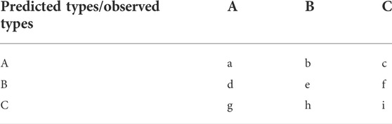
TABLE 2. An example of the error matrix of land cover classification.

4 Results

The random forest analysis provides the importance of waveform features for the urban land cover classification model and each land cover type. The variable importance of the random forest classification model can be expressed by the mean decrease in accuracy and mean decrease in Gini. We ranked the 22 waveform features according to their importance, as shown in Figure 4. Figure 4A shows that A_first has the largest mean decrease in accuracy, followed by ω_first, H_Eavg, nH_Eavg, R_Aω, SYM_S, S_rise, and ωR_{f_fl}. The other 14 features have an obviously smaller mean decrease in accuracy than these features. Figure 4B shows that A_first has the largest mean decrease in Gini, followed by ω_first, ωR_{f_fl}, SYM_S, R_Aω, H_Eavg, S_rise, and nH_Eavg. The remaining 14 features have an obviously smaller mean decrease in Gini than the above features. Therefore, A_first is the most important feature in urban land cover classification using waveform LiDAR features. Seven other features, namely, ω_first, H_Eavg, nH_Eavg, R_Aω, SYM_S, S_rise, and ωR_{f_fl}, also make important contributions to the classification results.

FIGURE 4

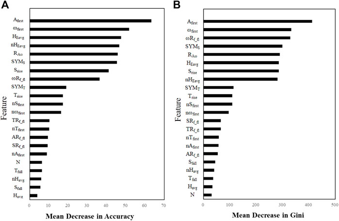
FIGURE 4. Variable importance of the urban land cover classification model in terms of mean decrease in accuracy (A) and mean decrease in Gini (B).

Table 3 shows the first six variables that are most important for each land cover type, in which the importance of variables decreases gradually from top to bottom. Table 3 shows that the peak amplitude of the first echo and its ratio to the echo width (i.e., A_first and R_Aω) effectively distinguish all types of land cover. Echo-width-related features (e.g., ω_first and ωR_{f_fl}) can be used to distinguish rough objects (e.g., tree and crop) from flat objects (e.g., buildings and impervious ground). Height-related features (e.g., nH_Eavg and H_Eavg) are important features in the classification of high objects (e.g., tree and high building), medium objects (e.g., low building), and low objects (e.g., bare soil and grass). Symmetry-related features (S_rise and SYM_S) can be used to distinguish objects with different vertical distribution characteristics (e.g., tree, crop, grass, high building, low building, and water).

TABLE 3

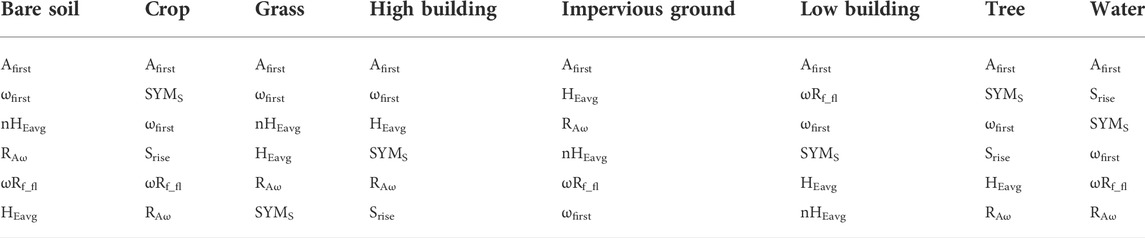
TABLE 3. The first six variables that are most important for each land cover type (ranking of importance from top to bottom).

We used the testing dataset to validate the accuracy of urban land cover classification. The confusion matrix is shown in Table 4. Table 4 shows that all land cover types have a producer’s accuracy of larger than 90% and a user’s accuracy of larger than 80%. Therefore, all land cover types are well classified. Among all land cover types, high building and water have the highest producer’s accuracy (97%), followed by tree (96.9%) and low building (94.6%). The impervious ground has the highest user accuracy (97.6%), followed by high building (97.3%), water (97.0%), and tree (96.7%). The overall accuracy of the urban land cover classification in this study region is 94.7%, and the kappa coefficient is 0.94.

TABLE 4

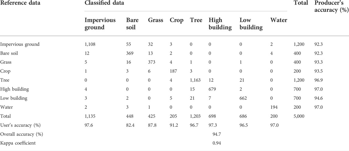
TABLE 4. Confusion matrix of the urban land cover classification results using a random forests classifier with waveform LiDAR features.

The land cover classification map of the study area using waveform features based on the random forest classification model is shown in Figure 5. Overall, the seven main land cover types (i.e., tree, high building, low building, impervious ground, grass, crop, and bare soil) were well depicted, and small water pools were also identified by the classification model. In addition, a comparison of Google Earth image and LiDAR-derived land cover classification results is shown in Figure 6, providing zoomed-in pictures of the detected trees and building borders. This comparison shows that full-waveform LiDAR data get good results for urban land cover classification in this study.

FIGURE 5

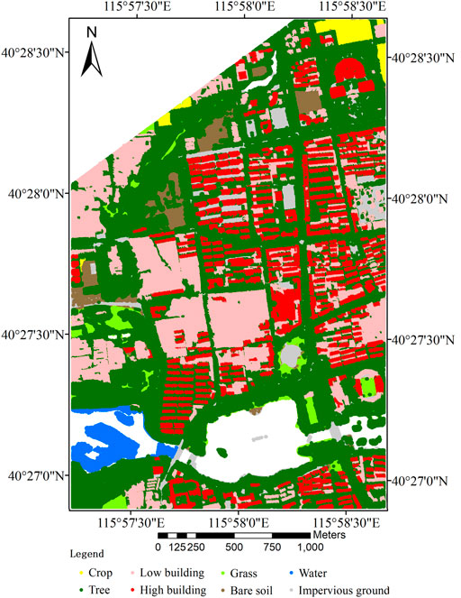
FIGURE 5. The urban land cover classification map of the study region.

FIGURE 6

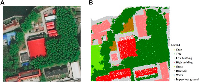
FIGURE 6. A comparison of Google Earth image (A) and LiDAR-derived land cover classification results (B).

5 Discussion

This study explored the ability of small-footprint full-waveform LiDAR data for urban land cover classification. Our results showed that the overall classification accuracy was 94.7%, and the kappa coefficient was 0.94. Therefore, the waveform LiDAR features proposed in this study provide an effective means for urban land cover classification using a random forest classifier. Among all waveform LiDAR features, the amplitude of the first echo plays the most important role in distinguishing all urban land cover types, which is consistent with a previous study (Mallet et al., 2011). Different land cover types have different reflection characteristics, so they have different amplitudes. The two new proposed amplitude-related variables, nA_first and A_{Rf_fl}, slightly influence urban land cover classification. Therefore, nA_first and A_{Rf_fl} cannot reflect the difference between the reflection characteristics of objects.

Echo width indicates surface roughness, object distribution, and surface slope due to the pulse broadening that occurs under these conditions. Large echo width corresponds to vegetation or other rough objects since they spread the LiDAR pulse. Small echo width is likely to correspond to flat ground and building. Among the three echo-width-related metrics, ω_first has the highest explanatory in classifying the eight urban land cover types, ωR_{f_fl} also plays an important role in classifying bare soil, crop, grass, impervious ground, low building, and water. The ratio of the amplitude and width of the first echo (R_Aω) is first proposed in this study. It can describe the waveform shape, representing the geometric and scattering characteristics of different land cover types. For example, vegetation often has smaller R_Aω than building and impervious ground. Therefore, R_Aω is an effective feature in classifying different urban land cover types.

Symmetry-related features can describe the symmetric of echoes, which are closely related to the spatial distribution and scattering characteristics of objects. These metrics were all first proposed in this study, and results showed that they have significant influences on identifying all urban land cover types. Vegetation and rough ground always have obvious asymmetries, whereas flat building, water, and impervious ground often have apparent symmetry. Height-related metrics can describe the height of an object, which can be used to distinguish objects with different heights effectively. H_Eavg and nH_Eavg are the two most important height features. Vertical-distribution-related variables can identify different land cover types to some degree, but they do not play an important role in urban land cover classification.

Previous studies have classified urban land cover types using airborne LiDAR data (Antonarakis et al., 2008; Yan et al., 2015). Zhou et al. (2013) classified four urban land cover types using height and intensity features derived from discrete-return LiDAR data and yielded an overall accuracy of 90.7%. Zhou et al. (2015) extracted distance, amplitude, waveform width, and backscattering cross-section from airborne full-waveform LiDAR data and used them to classify four land cover types, obtaining an overall accuracy of 79.57%. Tseng et al. (2015) extracted a series of individual echo and multi-echo features from full-waveform LiDAR data to classify five land cover types and achieved an overall accuracy of 86.01%. Compared with these studies, our study distinguished more urban land cover types and obtained higher classification accuracy. This may be because our study proposes many new features related to amplitude, echo width, mixed ratio, height, symmetry, and vertical distribution, which can provide more abundant object information.

Several studies have achieved higher classification accuracy than this study (Mallet et al., 2011; Azadbakht et al., 2018). For example, Mallet et al. (2011) extracted a series of features from waveform LiDAR data to classify building, ground, and vegetation and obtained an overall accuracy of 95.3%. The classification accuracy of this study is higher than that of our study because they only distinguished three land cover types, which was significantly less than that of our study. In addition, Azadbakht et al. (2018) combined sampling techniques and ensemble classifiers to classify 11 land cover types using full-waveform LiDAR data and obtained an overall accuracy of 97.4%. The higher classification accuracy obtained by this study is due to the higher density of LiDAR data they used, and the extracted features can be more refined in terms of object features.

Multi-return LiDAR can only record several echoes and obtain the three-dimensional coordinates and amplitude of each point. These features contain limited information, leading to insufficient classification types and low classification accuracy. In contrast, full-waveform LiDAR can record the entire waveform of the targets and obtain more features that can reflect the inherent characteristics of the target, such as the echo width, waveform shape, symmetry, and vertical distribution characteristics, which is helpful in improving its ability to classify urban land cover. These explanations have been well verified in this study. Therefore, it is necessary to continue to develop full-waveform LiDAR data acquisition and processing technology in the future to improve its ability in urban land cover classification and other applications.

6 Conclusion

In this study, we explored the ability of airborne small-footprint full-waveform LiDAR data for urban land cover classification. Eight land cover types were considered in this research: high building, low building, tree, grass, crop, impervious ground, bare soil, and water. We first proposed and extracted 22 waveform features from waveform LiDAR data, which are related to amplitude, echo width, mixed ratio, height, symmetry, and vertical distribution. Then, we assessed the feature importance and performed the urban land cover classification using a random forests classifier. In general, the urban land covers were well classified by these waveform features, resulting in an overall accuracy of 94.7% and a kappa coefficient of 0.94. We also found that A_first was the most important feature, and seven other features, namely, ω_first, H_Eavg, nH_Eavg, R_Aω, SYM_S, S_rise, and ωR_{f_fl}, also played important roles in urban land cover classification. Overall, airborne full-waveform LiDAR can accurately classify urban land cover types, and our proposed waveform features can improve the classification accuracy. Whether fusing full-waveform LiDAR and hyperspectral remote sensing imagery can improve the accuracy of urban land cover classification should be explored in the future.

Data availability statement

The raw data supporting the conclusion of this article will be made available by the authors without undue reservation.

Author contributions

HQ processed the data and wrote the draft. WZho proposed the concept and revised the manuscript. WZha revised the manuscript

Funding

This research was funded by the National Natural Science Foundation of China (Grant no. 32101292), the Research Center for Eco-Environmental Sciences, Chinese Academy of Sciences (Grant no. RCEES-TDZ-2021-9), and the Beijing Municipal Ecological and Environmental Monitoring Center (Grant no. 2241STC61348/01).

Conflict of interest

The authors declare that the research was conducted in the absence of any commercial or financial relationships that could be construed as a potential conflict of interest.

Publisher’s note

All claims expressed in this article are solely those of the authors and do not necessarily represent those of their affiliated organizations or those of the publisher, the editors, and the reviewers. Any product that may be evaluated in this article, or claim that may be made by its manufacturer, is not guaranteed or endorsed by the publisher.

References

Alexander, C., Tansey, K., Kaduk, J., Holland, D., and Tate, N. J. (2010). Backscatter coefficient as an attribute for the classification of full-waveform airborne laser scanning data in urban areas. ISPRS J. Photogrammetry Remote Sens. 65 (5), 423–432. doi:10.1016/j.isprsjprs.2010.05.002

CrossRef Full Text | Google Scholar

Antonarakis, A. S., Richards, K. S., and Brasington, J. (2008). Object-based land cover classification using airborne LiDAR. Remote Sens. Environ. 112 (6), 2988–2998. doi:10.1016/j.rse.2008.02.004

CrossRef Full Text | Google Scholar

Azadbakht, M., Fraser, C. S., and Khoshelham, K. (2018). Synergy of sampling techniques and ensemble classifiers for classification of urban environments using full-waveform LiDAR data. Int. J. Appl. Earth Observation Geoinformation 73, 277–291. doi:10.1016/j.jag.2018.06.009

CrossRef Full Text | Google Scholar

Breiman, L. (2001). Random forests. Mach. Learn. 45 (1), 5–32. doi:10.1023/a:1010933404324

CrossRef Full Text | Google Scholar

Chang, K-T., Yu, F-C., Chang, Y., Hwang, J-T., Liu, J-K., Hsu, W-C., et al. (2015). Land cover classification accuracy assessment using full-waveform LiDAR data. Terr. Atmos. Ocean. Sci. 26 (2-2), 169. doi:10.3319/tao.2014.12.02.02(eosi)

CrossRef Full Text | Google Scholar

Chen, F., Jiang, H., Van de Voorde, T., Lu, S., Xu, W., and Zhou, Y. (2018). Land cover mapping in urban environments using hyperspectral apex data: A study case in baden, Switzerland. Int. J. Appl. Earth Observation Geoinformation 71, 70–82. doi:10.1016/j.jag.2018.04.011

CrossRef Full Text | Google Scholar

Chen, Z., and Gao, B. (2014). An object-based method for urban land cover classification using airborne lidar data. IEEE J. Sel. Top. Appl. Earth Obs. Remote Sens. 7 (10), 4243–4254. doi:10.1109/jstars.2014.2332337

CrossRef Full Text | Google Scholar

Chiang, S-H., and Valdez, M. (2019). Tree species classification by integrating satellite imagery and topographic variables using maximum entropy method in a Mongolian forest. Forests 10 (11), 961. doi:10.3390/f10110961

CrossRef Full Text | Google Scholar

Dash, J., Mathur, A., Foody, G. M., Curran, P. J., Chipman, J. W., and Lillesand, T. M. (2007). Land cover classification using multi‐temporal MERIS vegetation indices. Int. J. Remote Sens. 28 (6), 1137–1159. doi:10.1080/01431160600784259

CrossRef Full Text | Google Scholar

Dong, W., Lan, J., Liang, S., Yao, W., and Zhan, Z. (2017). Selection of LiDAR geometric features with adaptive neighborhood size for urban land cover classification. Int. J. Appl. Earth Observation Geoinformation 60, 99–110. doi:10.1016/j.jag.2017.04.003

CrossRef Full Text | Google Scholar

Duong, V. H., Lindenbergh, R., Pfeifer, N., and Vosselman, G. (2008). Single and two epoch analysis of ICESat full waveform data over forested areas. Int. J. Remote Sens. 29 (5), 1453–1473. doi:10.1080/01431160701736372

CrossRef Full Text | Google Scholar

Gómez, C., White, J. C., and Wulder, M. A. (2016). Optical remotely sensed time series data for land cover classification: A review. ISPRS J. Photogrammetry Remote Sens. 116, 55–72. doi:10.1016/j.isprsjprs.2016.03.008

CrossRef Full Text | Google Scholar

Guo, L., Chehata, N., Mallet, C., and Boukir, S. (2011). Relevance of airborne lidar and multispectral image data for urban scene classification using Random Forests. ISPRS J. Photogrammetry Remote Sens. 66 (1), 56–66. doi:10.1016/j.isprsjprs.2010.08.007

CrossRef Full Text | Google Scholar

Hansen, M. C., Defries, R. S., Townshend, J. R. G., and Sohlberg, R. (2010). Global land cover classification at 1 km spatial resolution using a classification tree approach. Int. J. Remote Sens. 21 (6-7), 1331–1364. doi:10.1080/014311600210209

CrossRef Full Text | Google Scholar

Hellesen, T., and Matikainen, L. (2013). An object-based approach for mapping shrub and tree cover on grassland habitats by use of LiDAR and CIR orthoimages. Remote Sens. 5 (2), 558–583. doi:10.3390/rs5020558

CrossRef Full Text | Google Scholar

Immitzer, M., Atzberger, C., and Koukal, T. (2012). Tree species classification with random forest using very high spatial resolution 8-band WorldView-2 satellite data. Remote Sens. 4 (9), 2661–2693. doi:10.3390/rs4092661

CrossRef Full Text | Google Scholar

Jia, K., Liang, S., Zhang, N., Wei, X., Gu, X., Zhao, X., et al. (2014). Land cover classification of finer resolution remote sensing data integrating temporal features from time series coarser resolution data. ISPRS J. Photogrammetry Remote Sens. 93, 49–55. doi:10.1016/j.isprsjprs.2014.04.004

CrossRef Full Text | Google Scholar

Jiang, Y., Zhang, L., Yan, M., Qi, J., Fu, T., Fan, S., et al. (2021). High-resolution mangrove forests classification with machine learning using worldview and UAV hyperspectral data. Remote Sens. 13 (8), 1529. doi:10.3390/rs13081529

CrossRef Full Text | Google Scholar

Lee, H., Slatton, K. C., Roth, B. E., and Cropper, W. P. (2009). Prediction of forest canopy light interception using three‐dimensional airborne LiDAR data. Int. J. Remote Sens. 30 (1), 189–207. doi:10.1080/01431160802261171

CrossRef Full Text | Google Scholar

Luo, S., Wang, C., Xi, X., Zeng, H., Li, D., Xia, S., et al. (2015). Fusion of airborne discrete-return LiDAR and hyperspectral data for land cover classification. Remote Sens. 8 (1), 3. doi:10.3390/rs8010003

CrossRef Full Text | Google Scholar

Mallet, C., and Bretar, F. (2009). Full-waveform topographic lidar: State-of-the-art. ISPRS J. Photogrammetry Remote Sens. 64 (1), 1–16. doi:10.1016/j.isprsjprs.2008.09.007

CrossRef Full Text | Google Scholar

Mallet, C., Bretar, F., Roux, M., Soergel, U., and Heipke, C. (2011). Relevance assessment of full-waveform lidar data for urban area classification. Isprs J. Photogrammetry Remote Sens. 66 (6), S71–S84. doi:10.1016/j.isprsjprs.2011.09.008

CrossRef Full Text | Google Scholar

Man, Q., Dong, P., and Guo, H. (2015). Pixel- and feature-level fusion of hyperspectral and lidar data for urban land-use classification. Int. J. Remote Sens. 36 (6), 1618–1644. doi:10.1080/01431161.2015.1015657

CrossRef Full Text | Google Scholar

Myint, S. W., Gober, P., Brazel, A., Grossman-Clarke, S., and Weng, Q. (2011). Per-pixel vs. object-based classification of urban land cover extraction using high spatial resolution imagery. Remote Sens. Environ. 115 (5), 1145–1161. doi:10.1016/j.rse.2010.12.017

CrossRef Full Text | Google Scholar

Neuenschwander, A. L. (2009). Landcover classification of small-footprint, full-waveform lidar data. J. Appl. Remote Sens. 3 (1), 033544. doi:10.1117/1.3229944

CrossRef Full Text | Google Scholar

Paneque-Gálvez, J., Mas, J-F., Moré, G., Cristóbal, J., Orta-Martínez, M., Luz, A. C., et al. (2013). Enhanced land use/cover classification of heterogeneous tropical landscapes using support vector machines and textural homogeneity. Int. J. Appl. Earth Observation Geoinformation 23, 372–383. doi:10.1016/j.jag.2012.10.007

CrossRef Full Text | Google Scholar

Puertas, O. L., Brenning, A., and Meza, F. J. (2013). Balancing misclassification errors of land cover classification maps using support vector machines and Landsat imagery in the Maipo river basin (Central Chile, 1975-2010). Remote Sens. Environ. 137, 112–123. doi:10.1016/j.rse.2013.06.003

CrossRef Full Text | Google Scholar

Qin, Y., Li, S., Vu, T. T., Niu, Z., and Ban, Y. (2015). Synergistic application of geometric and radiometric features of LiDAR data for urban land cover mapping. Opt. Express 23 (11), 13761–13775. doi:10.1364/oe.23.013761

PubMed Abstract | CrossRef Full Text | Google Scholar

Raczko, E., and Zagajewski, B. (2017). Comparison of support vector machine, random forest and neural network classifiers for tree species classification on airborne hyperspectral APEX images. Eur. J. Remote Sens. 50 (1), 144–154. doi:10.1080/22797254.2017.1299557

CrossRef Full Text | Google Scholar

Rodriguez-Galiano, V. F., Ghimire, B., Rogan, J., Chica-Olmo, M., and Rigol-Sanchez, J. P. (2012). An assessment of the effectiveness of a random forest classifier for land-cover classification. ISPRS J. Photogrammetry Remote Sens. 67, 93–104. doi:10.1016/j.isprsjprs.2011.11.002

CrossRef Full Text | Google Scholar

Sherba, J., Blesius, L., and Davis, J. (2014). Object-based classification of abandoned logging roads under heavy canopy using LiDAR. Remote Sens. 6 (5), 4043–4060. doi:10.3390/rs6054043

CrossRef Full Text | Google Scholar

Sun, G., Ranson, K., Kimes, D., Blair, J., and Kovacs, K. (2008). Forest vertical structure from GLAS: An evaluation using LVIS and SRTM data. Remote Sens. Environ. 112 (1), 107–117. doi:10.1016/j.rse.2006.09.036

CrossRef Full Text | Google Scholar

Tseng, Y-H., Wang, C-K., Chu, H-J., and Hung, Y-C. (2015). Waveform-based point cloud classification in land-cover identification. Int. J. Appl. Earth Observation Geoinformation 34, 78–88. doi:10.1016/j.jag.2014.07.004

CrossRef Full Text | Google Scholar

Wagner, W., Ullrich, A., Ducic, V., Melzer, T., and Studnicka, N. (2006). Gaussian decomposition and calibration of a novel small-footprint full-waveform digitising airborne laser scanner. ISPRS J. Photogrammetry Remote Sens. 60 (2), 100–112. doi:10.1016/j.isprsjprs.2005.12.001

CrossRef Full Text | Google Scholar

Webster, R. BaT. L. (2006). Object oriented land cover classification of lidar derived surfaces. Can. J. Remote Sens. 32 (2), 162–172. doi:10.5589/m06-015

CrossRef Full Text | Google Scholar

Wu, M. F., Sun, Z. C., Yang, B., and Yu, S. S. (2016). A hierarchical object-oriented urban land cover classification using WorldView-2 imagery and airborne LiDAR data. IOP Conf. Ser. Earth Environ. Sci. 46, 012016. doi:10.1088/1755-1315/46/1/012016

CrossRef Full Text | Google Scholar

Wu, Q., Zhong, R., Zhao, W., Song, K., and Du, L. (2018). Land-cover classification using GF-2 images and airborne lidar data based on Random Forest. Int. J. Remote Sens. 40 (5-6), 2410–2426. doi:10.1080/01431161.2018.1483090

CrossRef Full Text | Google Scholar

Yan, W. Y., Shaker, A., and El-Ashmawy, N. (2015). Urban land cover classification using airborne LiDAR data: A review. Remote Sens. Environ. 158, 295–310. doi:10.1016/j.rse.2014.11.001

CrossRef Full Text | Google Scholar

Zhou, W., Huang, G., Troy, A., and Cadenasso, M. L. (2009). Object-based land cover classification of shaded areas in high spatial resolution imagery of urban areas: A comparison study. Remote Sens. Environ. 113 (8), 1769–1777. doi:10.1016/j.rse.2009.04.007

CrossRef Full Text | Google Scholar

Zhou, W. (2013). An object-based approach for urban land cover classification: Integrating LiDAR height and intensity data. IEEE Geosci. Remote Sens. Lett. 10 (4), 928–931. doi:10.1109/lgrs.2013.2251453

CrossRef Full Text | Google Scholar

Zhou, M., Liu, M., Zhang, Z., Ma, L., and Zhang, H. (2015). The research of land covers classification based on waveform features correction of full-waveform LiDAR. in SPIE Remote Sensing 9643, 96431. doi:10.1117/12.2193867

CrossRef Full Text | Google Scholar