 Steven F. Wilson
 Cliff Nietvelt2
 Shawn Taylor
95% of researchers rate our articles as excellent or good
Learn more about the work of our research integrity team to safeguard the quality of each article we publish.
Find out more
ORIGINAL RESEARCH article
Front. Environ. Sci. , 03 October 2022
Sec. Environmental Informatics and Remote Sensing
Volume 10 - 2022 | https://doi.org/10.3389/fenvs.2022.958596
This article is part of the Research Topic Application of Bayesian Modeling in Environmental Management View all 6 articles
The mountain goat (Oreamnos americanus) is an iconic wildlife species of western North America that inhabits steep and largely inaccessible terrain in remote areas. They are at risk from human disturbance, genetic isolation, climate change, and a variety of other stressors. Managing populations is challenging and mountain goats are particularly difficult and expensive to inventory. As a result, biologists often rely on models to estimate the species’ abundance and distribution in remote areas. We used landscape characteristics evident at point locations of mountain goat visual observations, tracks, and telemetry locations, along with random locations, to learn the structure and parameters of a Bayesian network that predicted the suitability of habitats for mountain goats. We then used the model to map habitat suitability across 285,000 km2 of potential habitat in mountain ranges of the south and central Canadian Pacific coast. Steep slopes, forest cover characteristics, and snow depth were the important drivers. Modeling the system as a Bayesian network provided several advantages over more common regression methods because input variables were heterogenous (i.e., a mix of discrete and continuous), autocorrelated, and animals exhibited non-linear responses to landscape conditions. These common characteristics of ecological data routinely violate the assumptions of parametric linear models, which are commonly used to map habitat suitability from animal observations.
Mountain goats (Oreamnos americanus) occur in mountainous terrain from southeast Alaska and southern Yukon and Northwest Territories in the north to Oregon, Idaho and Montana in the south, and have been introduced into sites in several US states (Myatt and Larkins, 2010). It is a species of particular interest in British Columbia (BC), where more than half of the global population resides and occupies most of the Province’s major mountain ranges (Shackleton, 2013).
Mountain goats are prominent in the cultures of First Nations peoples of BC, where the species’ wool was woven into blankets and clothing horns were fashioned into powder containers and utensils, while hides, skulls, and hooves were used in ceremonial regalia (Shackleton, 2013).
While globally secure, mountain goats in BC are ranked Special Concern, reflecting evidence of declining populations in some regions (BC Conservation Data Centre, 2022). While reasons for these declines are unclear, there are several factors that may be contributing, including loss of habitat and connectivity (Fox et al., 1989; Parks et al., 2015; Wolf et al., 2020), displacement from preferred habitat due to human-related disturbance (Côté, 1996; Cadsand, 2012), and climate-induced changes in mountain goat habitat (White et al., 2018). A key objective for the BC government is to maintain suitable, connected mountain goat habitat throughout the species’ range in the Province (BC Ministry of Environment, 2010).
Winter is a critical season for mountain goats because of the limited availability of food resources, higher vulnerability to predators, and increased energetic costs of moving through deep snow (Festa-Bianchet and Côté, 2008). The winter habitat use of mountain goats occupying ranges along the Pacific coast is unique because very deep, unconsolidated snowpacks force most goats to use low-elevation winter ranges, where old forest plays an important role in providing snow interception cover (Fox et al., 1989; Taylor et al., 2006; Taylor and Brunt, 2007). Moving inland from the coast, the snow packs become shallower and mountain goats transition from wintering primarily at low elevations to escape deep snow to wintering at higher elevations in areas that readily shed snow (Schoen and Kirchhoff, 1982).
Managing mountain goats in the Pacific ranges of BC is challenging because they occur at relatively low densities over large areas of largely remote and inaccessible terrain. As a result, biologists must rely on limited data to estimate the species’ abundance and to predict the distribution of important habitats to support conservation and management decisions.
Researchers have relied primarily on resource selection functions (RSFs; Manly, 2010) to model mountain goat habitat use and suitability (Lele and Keim, 2006; Taylor et al., 2006; White and Gregovich, 2017). This approach is common in studies of wildlife habitat selection (Boyce and McDonald, 1999; Burnham and Anderson, 2011; Fieberg et al., 2021). “Selection” is defined as use of a habitat unit disproportionately greater than its availability (Manly, 2010) and, typically, multiple logistic regression models are fit using a set of explanatory factors to a binary dependent variable of point observations of animals and random locations. Usually, “biologically plausible” candidate models, using different combinations of factors, are evaluated (Boyce et al., 2002) and then the most parsimonious model or set of models is selected, using an information-theoretic measure such as Akaike Information Criterion (AIC; Burnham and Anderson, 2011). RSF analyses need to meet the standard assumptions of parametric tests, which can be challenging with ecological data, where explanatory factors are often correlated and responses non-linear. Explanatory factors may also interact, although interaction terms are rarely included in candidate models.
RSFs have advanced in several respects over the years, most notably with the development of step-selection functions, which refines the habitat units considered “available” to wildlife as they move throughout their habitats (Thurfjell et al., 2014). While important, these advances have not addressed the underlying constraints that parametric, regression-based models impose on the evaluation and interpretation of habitat selection by wildlife.
In addition to RSFs, other analytical approaches are increasingly being employed in ecology and are particularly well-suited for characterizing complex non-linear relationships among covariates. Such models can generate high predictive accuracy, although often at the expense of transparency or the ability to interrogate the effects of individual factors (Ramazi et al., 2021).
Here, we applied a Bayesian network approach to model mountain goat winter habitat suitability in coastal BC to inform conservation and management strategies for the species, and to highlight potential benefits of the technique compared to RSFs. Bayesian networks are probabilistic graphical models that encode conditional dependencies among factors (Pearl, 2009). Conceptually straightforward and graphically presented, Bayesian networks are interpretable by a variety of audiences and, as a non-parametric approach, are not constrained by the same assumptions of regression-based models.
The study was conducted along the mainland coast of BC from the US border in the south to Tweedsmuir Provincial Park in the north, and inland to the eastern slopes of the Coast Mountains (Figure 1). The area covers approximately 285,000 km2 and is stratified into 130 mountain goat population units for management purposes. Terrain is generally rugged, except for some low-lying islands along the outer coast. Peaks of 2,000–3,000 m are common, rising steeply from numerous fjords that extend inland. Lower elevations are dominated by temperate rainforests with mixed stands of western hemlock (Tsuga heterophylla), western redcedar (Thuja plicata), and Sitka spruce (Picea sitchensis). Higher-elevation forests are dominated by mountain hemlock (Tsuga mertensiana), Pacific silver fir (Abies amabilis), and Alaska yellow-cedar (Callitropsis nootkatensis) stands, transitioning to Englemann spruce (Picea engelmannii) and subalpine fir (Abies lasiocarpa) forests in drier areas on the eastern slopes. Alpine is extensive, with low-lying ericaceous shrubs and expansive un-vegetated rock and glaciers. Rainfall varies between 1,000–5,000 mm annually, with 0–80% falling as snow in any given year, depending on elevation and latitude (Meidinger and Pojar, 1991).
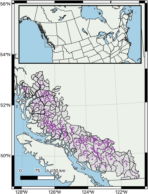
FIGURE 1. Study area in the Pacific coastal region of British Columbia, Canada. Population unit boundaries are illustrated, which served as the area over which the habitat suitability model was projected. Purple points illustrate the distribution of observations.
Data used in this study were retrieved from BC government databases and were collected via surveys and telemetry studies conducted between March 1990 and January 2022 (Figure 1). Mountain goats were surveyed by provincial government biologists during most years from helicopters in different parts of the region using various flightpaths and observers. At a minimum, the number of goats observed, or the presence of tracks were recorded, as well as the estimated geographic coordinates of the observations. Precision of observations was generally ±100 m.
Data also included telemetry locations from four research studies, including VHF-collared goats (n = 15) from the Kingcome drainage (51.2° E, -126.0° W) collected during 1994–1996 (Taylor and Brunt, 2007), GPS-collared goats (n = 24) from the Bute-Toba area (50.6° E, -124.4° W) studied from 2001–2003 (Taylor et al., 2006), GPS-collared goats (n = 2) on Mount Pauline (50.7° E, -123.0° W) from 2015–2017 (BC government, unpublished data), and GPS-collared goats (n = 31) from the vicinity of Meager Mountain (50.6° E, -123.6° W), 2018—January 2022 (Nietvelt, 2020; BC government unpublished data). There were 29,978 winter observations of mountain goats available for the analysis. Of these, 85% were GPS telemetry locations, 8% track observations, 6% visual observations, and the remainder VHF locations (<1%).
We included observation type in an initial model to check for bias in visual and track observations compared to telemetry points and found only that GPS telemetry locations occurred on average at higher elevations (expected value 1,270 ± 580 m) than tracks or visual observations (expected value 988 ± 560 m), based on the conditional probability distribution in the model. This was attributed primarily to bias in the distribution of GPS collared goats; only visual and track observations were available for some portions of the study area with the deepest snow and, consequently where goats wintered at the lowest elevations. In addition, fix rates of GPS collars are variable and accurate locations more difficult to acquire without a clear view of the sky, which is less likely to occur in low-elevation, forested valleys (Taylor et al., 2006). The network structure included no edges with other habitat factors and we elected to pool observation type in the final model by removing this node.
Location data from all sources were pooled from all studies; however, we ignored redundant locations in raster cells to avoid overfitting the model to high frequency GPS fixes. This resulted in evidence of use by goats in 13,295 raster locations. These observations were still spatially autocorrelated within our study area because of the distribution of sampling; however, subsampling to eliminate this autocorrelation and re-running our model did not substantially change our results and we therefore concluded that this spatial autocorrelation did not introduce significant bias.
Factors included in the model were selected to capture characteristics of habitat that are either known or suspected to be important to wintering coastal mountain goats, based on past research (Lele and Keim, 2006; Taylor et al., 2006; White and Gregovich, 2017) and in consultation with biologists who had experience with surveying or studying the species in the region. All factors were represented as 25 by 25-m raster cells and projected in NAD83/BC Albers (EPSG:3005) for model processing. The following were the factors included in the model:
Distance to escape terrain: non-vegetated areas from the BC Vegetation Resources Inventory data (https://www2.gov.bc.ca/gov/content/industry/forestry/managing-our-forest-resources/forest-inventory) and slopes 30–60° were used to characterize potential escape terrain. The variable was discretized into four classes for model building: 0 m (i.e., the point location was within escape terrain), ≤150 m, 151–300 m, and >300 m (Hamel and Côté, 2008).
Elevation: Elevation was derived from a 25-m resolution Digital Elevation Model (DEM) and discretized into the following classes: ≤500 m, 501–900 m, 901–1,300 m, 1,301–1700 m and >1700 m.
Forest age class: Forest cover was derived from Vegetation Resources Inventory data (https://www2.gov.bc.ca/gov/content/industry/forestry/managing-our-forest-resources/forest-inventory) and discretized into the following classes: Early (0–40 years), Mid (41–80 years), Mature (81–140 years), Old (>141 years), and Non-forested. These data are derived from photo interpretation and are subject to unknown classification error, particularly at higher elevations and in remote areas. Current habitat conditions might not match those that existed at the time of some older observations, due to forest harvesting or aging of the forest. Older forests intercept more snow and are correlated with lower snow depths under canopy (Kirchhoff and Schoen, 1987). Data on canopy closure were not available for all areas and therefore could not be used in the model.
Snow zone: Broad snow zones were interpreted from the characteristics of different ecosystem zones. Snow zones were assigned to unique biogeoclimatic subzone variants, which is a level of the Biogeoclimatic Ecosystem Classification system developed by the Government of BC (https://www.for.gov.bc.ca/hre/becweb/). Documentation for each subzone variant in the study area was reviewed and assigned a snow zone based on the description of the local climate and precipitation characteristics (see Supplemental Material).
We used the following snow zone definitions:
1. Shallow: snow usually <30 cm and ephemeral;
2. Moderate: persistent winter snow, usually shallow (30–100 cm) with occasional periods of deep snow (>1 m);
3. Deep: persistent, deep (>1 m) snow for the entire winter, with periods of very deep snow (>3 m)
4. Very deep: very deep (>3 m) snow for the entire winter, with snow cover in most years in early fall through late spring, with common, permanent snowfields and glaciers in some areas.
Other model inputs were assumed to modify these broad snow zones to reflect local snow conditions (i.e., elevation, slope, and solar insolation).
Slope: Slope was derived from the DEM and was discretized into the following classes: ≤35%, 36–100%, and >100%.
Solar insolation: Solar insolation was calculated from the DEM as well as from latitude using the ArcGIS Area Solar Radiation script (https://pro.arcgis.com/en/pro-app/latest/tool-reference/spatial-analyst/area-solar-radiation.htm). Units are kW hours per square meter (kWh/m2).
Bayesian networks are directed acyclic graphs (DAGs) composed of nodes connected by directed edges. Each node encodes a random variable as a series of discrete states and the edges represent the conditional dependencies amongst variables (Marcot et al., 2006). The probability distribution of states within a node is determined by the probability distributions of the node’s “parents” upstream in the network. The joint probability distributions are derived fundamentally from Bayes Rule:
That is, the joint probability of both a and b occurring is the conditional probability of a occurring given that b occurred, multiplied by the probability of b occurring. This specific case of two variables is extended to n variables via the chain rule (Heckerman, 2022):
That is, the joint probability distribution for a node x is equal to the product of the probability of each state xi of the node, given all the parents of xi.
When “evidence” is entered for any node in the network (i.e., the probability distribution for a node is revised in some way), the chain rule propagates the evidence throughout the network and updates the probability distributions for all the connected nodes in a manner consistent with Bayes Rule. In our application, the “target“ node for updating is the one that predicts the habitat suitability of a map raster based on various predicting factors represented as other nodes in the network.
Structural learning is the process of determining the configuration of edges based on learning data associated with each node. There are many different structural learning algorithms that all attempt to represent the joint probability distribution of the network through a parsimonious configuration of edges (Friedman et al., 1997). Following structural learning, the data set is again used to learn the distributions for all of the states within all of the nodes of the network. This is accomplished by finding the maximum likelihood network, which is the set of parameters that is the most likely, given the data. Expectation maximization (EM) is the algorithm most often employed (Do and Batzoglou, 2008). Finally, a set of evidence data, in our case representing the value of each habitat variable at each pixel in our study area, is run through the model to infer the habitat suitability.
For our application, we used a binary target variable, with a class representing locations with evidence of goat use and a class representing random locations within the study area. We used the same number of random locations as observations to prevent overfitting to one class or the other. The random locations were drawn from the distributions of all the predictor variables to ensure that they reflected the composition of the study area.
The network structure was fit using the Sons and Spouses classifier (Madden, 2009). This classifier is similar to the tree-augmented Naïve Bayes classifier (Friedman et al., 1997) but allows for relationships not directly linked to the response node (Costello et al., 2020). The joint probability distribution (i.e., the frequencies associated with the marginal or conditional probability tables of each node) was then fit using expectation maximization (Bilmes, 1998). Probabilities of >50% of being classified as an observation (as opposed to a random location) were interpreted as evidence of habitat selection (Wilson and DeMars, 2015).
Model fit was assessed using k-fold (k = 10) cross-validation (Fielding and Bell, 1997), the Receiver Operating Characteristic (ROC) index (Nakas et al., 2003), and by examining the ratio of correct predictions to the total number of observations in resulting confusion matrices.
Input data were run through the model, with each mapped 25-m pixel corresponding to a case of the six inputs, and the output probability of selection was then mapped across the study area. The predicted habitat suitability of each observation was ordered and then binned based on proportion, such that, for example, locations within the study area with a predicted suitability equal to or greater than the 25% of observations with the highest suitability were considered to be the most suitable habitat (“best 25%“). This was repeated for the best 50, 75, and 95%.
Spatial processing employed QGIS 3.26 (QGIS Association) and modeling was conducted in BayesiaLab 10.2 (Bayesia S.A.S., Laval, France). Landscape metrics were calculated using R version 4.0.5 and library landscapemetrics 1.5.4 (Hesselbarth et al., 2019).
Sites used by goats occurred overwhelmingly in old forest or non-forested areas and on moderate-steep slopes (Figure 2). More than 87% were located at elevations between 900 and 1,700 m, and approximately 75% were in moderate and deep snow zones. About 65% of sites were located <300 m from escape terrain and in areas of high solar insolation. Most of the study area (but proportionally smaller than used sites) is also composed of either old forest or non-forested areas, farther from escape terrain, on shallower slopes, and in areas of less solar insolation (Figure 3). Elevational bands and snow zones were distributed relatively equally throughout the study area.
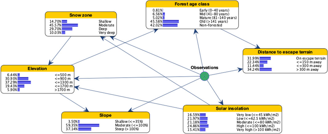
FIGURE 2. Bayesian network model of mountain goat winter range for coastal British Columbia, Canada, illustrating the distribution of states for input variables when setting evidence on observations.
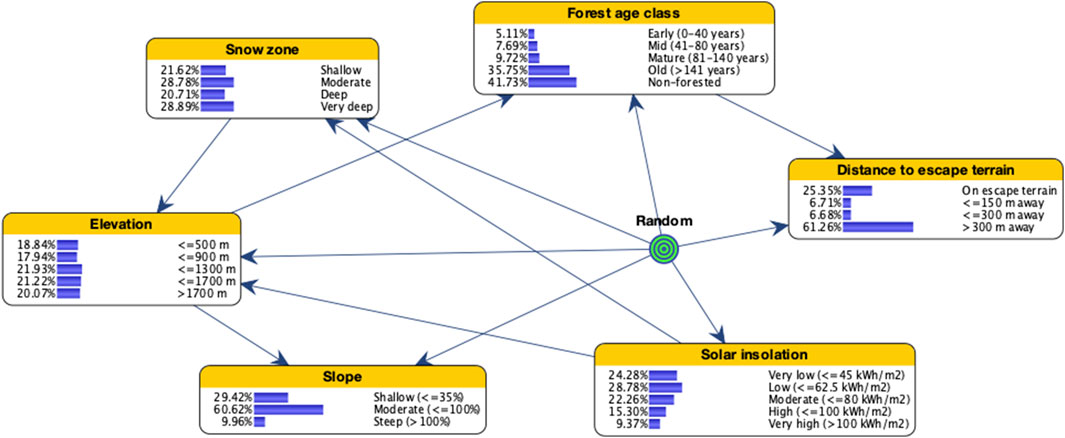
FIGURE 3. Bayesian network model of mountain goat winter range for coastal British Columbia, Canada, illustrating the distribution of states for input variables when setting evidence on random points.
K-folds cross-validation indicated a good fit of the final model with an ROC index of 95.0% (Figure 4) and a mean precision (percentage of points correctly classified by the model) of 90.8% for observations and 85.5% for random locations. The mean reliability (percentage of modelled locations correctly classified) was 86.3% for observations and 90.3% for random locations.
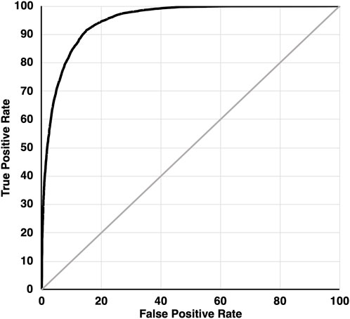
FIGURE 4. Receiver Operator Characteristic (ROC) curve illustrating the goodness-of-fit of the mountain goat winter habitat suitability model, plotting the rate of true positives against false positives for the target variable classifying observations versus random points under different discrimination thresholds.
In addition to the relationships between the target node and the explanatory factors, there were also significant relationships among some of the explanatory factors (Table 1). For example, elevation was correlated with snow zone (r = 0.27) and solar insolation (r = 0.20), while forest age class was correlated with distance to escape terrain (r = -0.16) because of the coincidence of non-forested and non-vegetated areas.
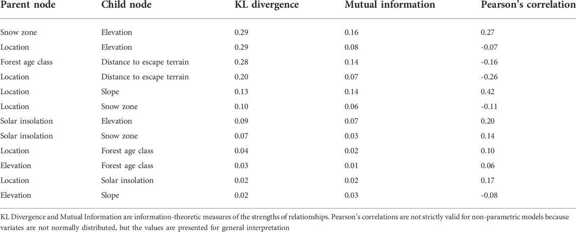
TABLE 1. Relationships among nodes in the mountain goat winter habitat suitability model.
The model was most sensitive to changes in slope, forest age class, and snow zone, followed by solar insolation, distance to escape terrain, and elevation (Figure 5). The final model identified 69,675 km2 of potential mountain goat habitat broadly distributed throughout the study area, but more concentrated in the mid-coast region, with only 0.7% corresponding to the highest 25% habitat suitability (Figure 6). High suitability patches were generally small with a patch cohesion index of 87.6% (Schumaker, 1996). The habitat capturing the best 50% estimated suitability covered 6.8% of the potential habitat with a patch cohesion index of 96.9%.
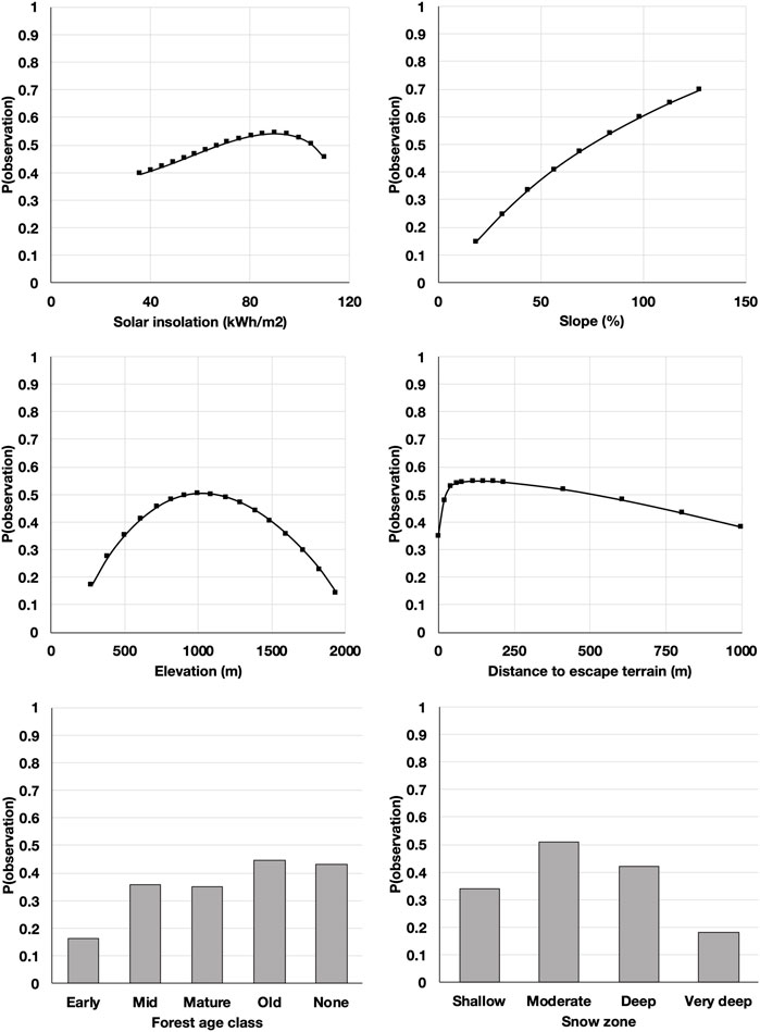
FIGURE 5. Independent (direct) effects of model input variables on the probability of a point being classified as an observation or a random location, based on soft evidence (Peng et al., 2010). Probabilities above 0.5 indicate habitat selection. Steeper slopes indicate a stronger effect size.
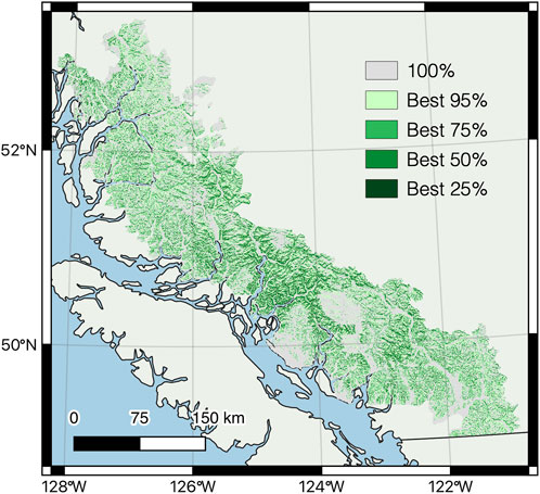
FIGURE 6. Mountain goat winter habitat suitability in coastal British Columbia, Canada, based on the probability of selection estimated by the Bayesian network analysis of observations versus random locations. Modelled habitat suitability for each observation was ranked from highest to lowest and classes reflect the suitability of habitat in which different proportions of observations were located (e.g., the 25% of telemetry locations with the highest habitat suitability we’re located in areas modelled in the darkest green).
This project extends the application of Bayesian networks to a common application in wildlife conservation and management; namely, modeling habitat selection and mapping habitat suitability. RSFs are commonly used for generating such models for mountain goats (e.g., Taylor et al., 2006; White and Gregovich, 2017).
Despite its widespread use, multiple logistic regression is not an ideal statistical model for estimating habitat selection. First, the dependent variable in a logistic regression is assumed to be binary; however, data used for analyses are usually not stratified into “used” and “unused” units, but rather into “used” and “available” units. As a result, some subset of the “available” units are likely to have been “used.” This is referred to as “zero contamination” and generates bias in estimates (Johnson et al., 2006). Care must be exercised in analyses to accommodate these “pseudoabsences” (Avgar et al., 2017). Our Bayesian approach makes no explicit claim about “unused” units and instead models the contrast between “used” and “available” units directly.
The definition of habitat “available” to animals has itself been a focus of research, because analyses of habitat selection are influenced as much by the characterization of what is considered “available” as by what animals use (Northrup et al., 2013). We used a simple characterization that considered the entire study area as “available.” We based this decision on the intended broad-scale interpretation and application of the resulting model for regional planning purposes. That is, the model is intended to be used to stratify the land base into areas of different habitat suitability for mountain goats, rather than to understand habitat selection decisions of individuals at a home range scale. This latter approach would have demanded a different strategy for defining “available” habitat (e.g., step-selection functions; Thurfjell et al., 2014).
Second, Bayesian networks can accommodate mixes of continuous (if discretized), ordinal, and categorical variables in the same network. Accommodating different data types in regression can be awkward and complicates interpretation. For example, categorical variables must be coded as a series of dummy variables and interpreted in relation to a reference category that is excluded from the function.
Third, multiple logistic regression is supposed to meet the standard assumptions of parametric analyses, including no multicollinearity among explanatory variables, and a linear relationship between the explanatory variables and the logit of the response variable. These assumptions are rarely met in ecological systems and are usually addressed by omitting highly correlated explanatory variables and applying transformations to linearize relationships. These adjustments are unnecessary when fitting non-parametric Bayesian networks because they can represent any arbitrary relationship among variables as conditional dependencies. As a result, the effect of any subset of explanatory variables on the response variable can be computed in such a structure (Ramazi et al., 2021). Non-linearities were observed in the response of mountain goats to several explanatory variables in this study and modeling these variables directly rather than applying transformations simplified interpretation.
Fourth, the output of a Bayesian network is relatively simple to interpret for a variety of audiences. Network diagrams, illustrating connections among key variables are more accessible than equations (Ramazi et al., 2021), and the probabilistic relationships are easier to interpret than the tables of raw or standardized regression coefficients that are usually presented.
Finally, there is little guidance on how “biologically plausible” candidate models should be structured in such an analysis. Specifically, which highly correlated factors should be omitted? Which interactions should be included? How many competing models should be evaluated and what constitutes sufficient evidence of support and what if several models meet that threshold? These decisions, along with the issues listed above, can lead to analysis results that can be more obfuscating than illuminating. The issues increase as more explanatory variables are added. The Bayesian network approach can accommodate more complex model structures than can be accommodated in regression equations and requires fewer a priori decisions regarding alternative model structures to be tested.
Of course, generating a Bayesian network still requires decisions regarding which explanatory variables to include initially, learning algorithms to apply (Acid et al., 2004), and decisions regarding discretization of continuous variables (Bertens et al., 2012; Nojavan et al., 2017). Learning Bayesian networks also tends to require large sample sizes to minimize the risk of bias generated by sparse joint probability distributions (Wocjan et al., 2002). However, on balance the Bayesian approach requires fewer adjustments and decisions and generates more interpretable results than using a regression-based approach.
The output of our mountain goat winter habitat suitability model generally aligned with the results of other studies of winter habitat selection. Steep slopes, escape terrain, and solar insolation are key characteristics of suitable mountain goat habitat in this critical season (e.g., Taylor et al., 2006; Festa-Bianchet and Côté, 2008; Wolf et al., 2022). In addition, old forest with relatively dense canopies is important for coastal populations where deep, unconsolidated snow drives mountain goats to lower elevations in seek of lower snow loads and accessible forage (Shackleton, 2013; White and Gregovich, 2017). Our study area also included areas consistent with more interior climatic conditions where mountain goats typically winter at high elevations (e.g., Wolf et al., 2022). The model identified suitable habitat associated with both strategies, as well as transitional areas.
Because Bayesian networks formulate the joint probability structure, they are well-suited for interrogating models about the effects of individual factors or subsets of factors on the response variable, even where factors are correlated (Ramazi et al., 2021). For example, setting evidence on the Bayesian model suggested that old forest on moderate slopes in the low snow zone is generally avoided by mountain goats (probability of selection 40%); however, in the deep snow zone, such areas are selected (probability of selection 68%). So, while our model identified a set of important predictor variables that was similar to other studies, it presents an opportunity to better discriminate the contributions of those predictors to the observed patterns of habitat use.
Although most often used to model species’ distributions rather than habitat suitability, MaxEnt is a “presence-only” approach to mapping probability of occupancy and defines available habitat similarly to our model and shares some similar advantages, such as the ability to model non-linear responses (Merow et al., 2013); however, MaxEnt models require that the model structure be fully described a priori and the response of the target variable to changes in individual factors or subsets of factors cannot be estimated (Ramazi et al., 2021).
Our model was likely affected by limitations in our source data, which included repeated sampling on GPS-collared goats in spatially limited portions of the study area during relatively short time frames, as well as more spatially widespread visual observations and tracks on unknown individuals over decades. We mitigated the effect of frequent GPS samples by removing redundant observations in each cell, and our results were robust to the spatial autocorrelation exhibited by our observations. Still, sampling bias remains a risk because there were portions of the study area that were under-sampled (e.g., no telemetry studies conducted and few or no aerial surveys).
The model has subsequently been used to assess the effectiveness of current protected areas established for wintering mountain goats, to identify additional areas of suitable habitat that might be occupied, and to generate preliminary habitat-based population estimates and objectives. Other potential uses could involve analyzing habitat connectivity and forecasting future changes in habitat suitability under different management regimes and expected shifts in snow zones with climate change. Future survey data will be used to validate and further refine the model, and a similar approach is planned for the development of a summer habitat model.
Because our Bayesian network approach generated results similar to previous studies based on RSFs, our support for this method is driven primarily by its apparent theoretical advantages and its interpretability, rather than by a conclusion that RSFs are inappropriate for modeling our system. We suggest that these advantages become more important as the number and interrelationships among explanatory variables grows, and with an increasing diversity of data types. This makes Bayesian networks an attractive alternative for researchers and may offer advantages over RSFs, depending on the specifics of the systems studied.
The data analyzed in this study is subject to the following licenses/restrictions: Data analyzed were from a variety of sources and funders, and limited use was granted for this study. Some data are publicly available from the Government of British Columbia. Requests to access these datasets should be directed to daniel.guertin@gov.bc.ca.
SW and DG contributed to conception and design of the study. SW conducted the modeling and drafted the manuscript. CN and ST developed, directed, and conducted field data collection. All authors contributed to manuscript revision, read, and approved the submitted version.
This work was provided by the British Columbia Conservation Foundation Project #8102062 and by the Government of British Columbia.
Model development and revision benefitted from discussions with, and feedback from: Nicola Bickerton, Steve Gordon, Bill Jex, John Kelly, Josh Malt, Darryn McConkey, Carl Morrison, Kyle Rezansoff, Tania Tripp, and Steve Rochetta. Ada Li managed data compilation.
The authors declare that the research was conducted in the absence of any commercial or financial relationships that could be construed as a potential conflict of interest.
All claims expressed in this article are solely those of the authors and do not necessarily represent those of their affiliated organizations, or those of the publisher, the editors and the reviewers. Any product that may be evaluated in this article, or claim that may be made by its manufacturer, is not guaranteed or endorsed by the publisher.
The Supplementary Material for this article can be found online at: https://www.frontiersin.org/articles/10.3389/fenvs.2022.958596/full#supplementary-material
Acid, S., de Campos, L. M., Fernández-Luna, J. M., Rodrı́guez, S., Marı́a Rodrı́guez, J., and Luis Salcedo, J. (2004). A comparison of learning algorithms for bayesian networks: A case study based on data from an emergency medical service. Artif. Intell. Med. (2017). 30, 215–232. doi:10.1016/j.artmed.2003.11.002
Avgar, T., Lele, S. R., Keim, J. L., and Boyce, M. S. (2017). Relative Selection Strength: Quantifying effect size in habitat‐ and step‐selection inference. Ecol. Evol. 7, 5322–5330. doi:10.1002/ece3.3122
BC Ministry of Environment (2010). Management plan for the mountain goat (Oreamnos americanus) in British Columbia. Victoria, BC: BC Ministry of Environment.
Bertens, R., van der Gaag, L. C., and Renooij, S. (2012). “Discretisation effects in naive bayesian networks,” in Advances in computational intelligence communications in computer and information science. Editors S. Greco, B. Bouchon-Meunier, G. Coletti, M. Fedrizzi, B. Matarazzo, and R. R. Yager (Berlin, Heidelberg: Springer Berlin Heidelberg), 161–170. doi:10.1007/978-3-642-31718-7_17
Bilmes, J. A. (1998). A gentle tutorial of the EM algorithm and its application to parameter estimation for Gaussian mixture and hidden Markov models. Int. Comput. Sci. Inst. 4, 126.
Boyce, M. S., and McDonald, L. L. (1999). Relating populations to habitats using resource selection functions. Trends Ecol. Evol. 14, 268–272. doi:10.1016/S0169-5347(99)01593-1
Boyce, M. S., Vernier, P. R., Nielsen, S. E., and Schmiegelow, F. K. A. (2002). Evaluating resource selection functions. Ecol. Modell. 157, 281–300. doi:10.1016/S0304-3800(02)00200-4
Burnham, K. P., and Anderson, D. R. (2011). Model selection and multi-model inference: A practical information-theoretic approach. New ed. New York London: Springer.
Cadsand, B. A. (2012). Response of mountain goats to heliskiing activity: Movements and resource selection.
Costello, F. J., Kim, C., Kang, C. M., and Lee, K. C. (2020). Identifying high-risk factors of depression in middle-aged persons with a novel sons and spouses Bayesian network model. Healthcare 8, 562. doi:10.3390/healthcare8040562
Côté, S. D. (1996). Mountain goat responses to helicopter disturbance. Wildl. Soc. Bull. 24, 681–685.
Do, C. B., and Batzoglou, S. (2008). What is the expectation maximization algorithm? Nat. Biotechnol. 26, 897–899. doi:10.1038/nbt1406
Festa-Bianchet, M., and Côté, S. D. (2008). Mountain goats: Ecology, behavior, and conservation of an alpine ungulate. Washington, DC: Island Press.
Fieberg, J., Signer, J., Smith, B., and Avgar, T. (2021). A ‘How to’ guide for interpreting parameters in habitat‐selection analyses. J. Anim. Ecol. 90, 1027–1043. doi:10.1111/1365-2656.13441
Fielding, A. H., and Bell, J. F. (1997). A review of methods for the assessment of prediction errors in conservation presence/absence models. Environ. Conserv. 24, 38–49. doi:10.1017/S0376892997000088
Fox, J. L., Smith, C. A., and Schoen, J. W. (1989). Relation between mountain goats and their habitat in southeastern Alaska. Portland, OR: US Department of Agriculture Forest Service. Pacific Northwest Research Station.
Friedman, N., Geiger, D., and Goldszmidt, M. (1997). Bayesian network classifiers. Mach. Learn. 29, 131–163. doi:10.1023/a:1007465528199
Hamel, S., and Côté, S. D. (2008). Trade-offs in activity budget in an alpine ungulate: Contrasting lactating and nonlactating females. Anim. Behav. 75, 217–227. doi:10.1016/j.anbehav.2007.04.028
Heckerman, D. (2022). A tutorial on learning with bayesian networks. Available at: http://arxiv.org/abs/2002.00269 (Accessed August 26, 2022).
Hesselbarth, M. H. K., Sciaini, M., With, K. A., Wiegand, K., and Nowosad, J. (2019). Landscapemetrics : an open‐source R tool to calculate landscape metrics. Ecography 42, 1648–1657. doi:10.1111/ecog.04617
Johnson, C. J., Nielsen, S. E., Merrill, E. H., Mcdonald, T. L., and Boyce, M. S. (2006). Resource selection functions based on use–availability data: Theoretical motivation and evaluation methods. J. Wildl. Manag. 70, 347–357. doi:10.2193/0022-541X(2006)70[347:RSFBOU]2.0.CO;2
Kirchhoff, M. D., and Schoen, J. W. (1987). Forest cover and snow: Implications for deer habitat in southeast Alaska. J. Wildl. Manage. 51, 28–33. doi:10.2307/3801623
Lele, S. R., and Keim, J. L. (2006). Weighted distributions and estimation of resource selection probability functions. Ecology 87, 3021–3028. doi:10.1890/0012-9658(2006)87[3021:wdaeor]2.0.co;2
Madden, M. G. (2009). On the classification performance of TAN and general Bayesian networks. Knowl. Based. Syst. 22, 489–495. doi:10.1016/j.knosys.2008.10.006
Manly, B. F. J. (2010). Resource selection by animals: Statistical design and analysis for field studies, 2. Dordrecht: Kluwer. reprint.
Marcot, B. G., Steventon, J. D., Sutherland, G. D., and McCann, R. K. (2006). Guidelines for developing and updating Bayesian belief networks applied to ecological modeling and conservation. Can. J. For. Res. 36, 3063–3074. doi:10.1139/x06-135
Meidinger, D., and Pojar, J. (1991). . “Ecosystems of British Columbia,” in . Spec. Rep. Ser. Victoria, BC: Minist. For..
Merow, C., Smith, M. J., and Silander, J. A. (2013). A practical guide to MaxEnt for modeling species’ distributions: What it does, and why inputs and settings matter. Ecography 36, 1058–1069. doi:10.1111/j.1600-0587.2013.07872.x
Myatt, N., and Larkins, A. N. (2010). Mountain goats in north America: A survey of population status and management. Bienn. Symp. North. Wild Sheep Goat Counc. 17, 1–7.
Nakas, C., Yiannoutsos, C. T., Bosch, R. J., and Moyssiadis, C. (2003). Assessment of diagnostic markers by goodness-of-fit tests. Stat. Med. 22, 2503–2513. doi:10.1002/sim.1464
Nietvelt, C. (2020). Mountain goat seasonal movements and habitat use in the Mount Meager complex, South Coast: Year 2 update. Victoria, BC: Habitat Conservation Trust Foundation.
Nojavan, A., F., Qian, S. S., and Stow, C. A. (2017). Comparative analysis of discretization methods in Bayesian networks. Environ. Model. Softw. 87, 64–71. doi:10.1016/j.envsoft.2016.10.007
Northrup, J. M., Hooten, M. B., Anderson, C. R., and Wittemyer, G. (2013). Practical guidance on characterizing availability in resource selection functions under a use–availability design. Ecology 94, 1456–1463. doi:10.1890/12-1688.1
Parks, L. C., Wallin, D. O., Cushman, S. A., and McRae, B. H. (2015). Landscape-level analysis of mountain goat population connectivity in Washington and southern British Columbia. Conserv. Genet. 16, 1195–1207. doi:10.1007/s10592-015-0732-2
Pearl, J. (2009). “Probabilistic reasoning in intelligent systems: Networks of plausible inference. Rev. 2,” in Transferred to digital printing (San Francisco, Calif: Morgan Kaufmann).
Peng, Y., Zhang, S., and Pan, R. (2010). Bayesian network reasoning with uncertain evidences. Int. J. Unc. Fuzz. Knowl. Based. Syst. 18, 539–564. doi:10.1142/S0218488510006696
Ramazi, P., Kunegel‐Lion, M., Greiner, R., and Lewis, M. A. (2021). Exploiting the full potential of Bayesian networks in predictive ecology. Methods Ecol. Evol. 12, 135–149. doi:10.1111/2041-210X.13509
Schoen, J. W., and Kirchhoff, M. D. (1982). Habitat use by mountain goats in southeast Alaska. Juneau, AK: Alaska Department of Fish and Game.
Schumaker, N. H. (1996). Using landscape indices to predict habitat connectivity. Ecology 77, 1210–1225. doi:10.2307/2265590
Taylor, S., and Brunt, K. (2007). Winter habitat use by mountain goats in the Kingcome River drainage of coastal British Columbia. J. Ecosyst. Manag. 8.
Taylor, S., Wall, W., and Kulis, Y. (2006). Habitat selection by mountain goats in south coastal British Columbia. Bienn. Symp. North. Wild Sheep Goat Counc. 25, 141–157.
Thurfjell, H., Ciuti, S., and Boyce, M. S. (2014). Applications of step-selection functions in ecology and conservation. Mov. Ecol. 2, 4. doi:10.1186/2051-3933-2-4
White, K. S., Gregovich, D. P., and Levi, T. (2018). Projecting the future of an alpine ungulate under climate change scenarios. Glob. Change Biol. 24, 1136–1149. doi:10.1111/gcb.13919
White, K. S., and Gregovich, D. P. (2017). Mountain goat resource selection in relation to mining-related disturbance. Wildl. Biol. 2017, 1–12. doi:10.2981/wlb.00277
Wilson, S. F., and Demars, C. A. (2015). A Bayesian approach to characterizing habitat use by, and impacts of anthropogenic features on, woodland caribou (Rangifer tarandus caribou) in northeast British Columbia. Can. Wildl. Biol. Manag. 4, 107–118.
Wocjan, P., Janzing, D., and Beth, T. (2002). Required sample size for learning sparse Bayesian networks with many variables. Available at: http://arxiv.org/abs/cs/0204052 (Accessed May 24, 2022).
Wolf, J. F., Kriss, K. D., MacAulay, K. M., and Shafer, A. B. A. (2020). Panmictic population genetic structure of northern British Columbia mountain goats (Oreamnos americanus) has implications for harvest management. Conserv. Genet. 21, 613–623. doi:10.1007/s10592-020-01274-6
Keywords: Bayesian networks, habitat suitability, mountain goats (Oreamnos americanus), British Columbia (BC), wildlife management
Citation: Wilson SF, Nietvelt C, Taylor S and Guertin DA (2022) Using Bayesian networks to map winter habitat for mountain goats in coastal British Columbia, Canada. Front. Environ. Sci. 10:958596. doi: 10.3389/fenvs.2022.958596
Received: 31 May 2022; Accepted: 15 September 2022;
Published: 03 October 2022.
Edited by:
Elena Moltchanova, University of Canterbury, New ZealandReviewed by:
Kevin White, Div of Wildlife Conservation (retired), Haines, AK, United StatesCopyright © 2022 Wilson, Nietvelt, Taylor and Guertin. This is an open-access article distributed under the terms of the Creative Commons Attribution License (CC BY). The use, distribution or reproduction in other forums is permitted, provided the original author(s) and the copyright owner(s) are credited and that the original publication in this journal is cited, in accordance with accepted academic practice. No use, distribution or reproduction is permitted which does not comply with these terms.
*Correspondence: Steven F. Wilson, c3RldmVuLndpbHNvbkBlY29sb2dpY3Jlc2VhcmNoLmNh
Disclaimer: All claims expressed in this article are solely those of the authors and do not necessarily represent those of their affiliated organizations, or those of the publisher, the editors and the reviewers. Any product that may be evaluated in this article or claim that may be made by its manufacturer is not guaranteed or endorsed by the publisher.
Research integrity at Frontiers
Learn more about the work of our research integrity team to safeguard the quality of each article we publish.