For the aged: A novel PM2.5 concentration forecasting method based on spatial-temporal graph ordinary differential equation networks in home-based care parks

The immune ability of the elderly is not strong, and the functions of the body are in a stage of degeneration, the ability to clear PM2.5 is reduced, and the cardiopulmonary system is easily affected. Accurate prediction of PM2.5 can provide guidance for the travel of the elderly, thereby reducing the harm of PM2.5 to the elderly. In PM2.5 prediction, existing works usually used shallow graph neural network (GNN) and temporal extraction module to model spatial and temporal dependencies, respectively, and do not uniformly model temporal and spatial dependencies. In addition, shallow GNN cannot capture long-range spatial correlations. External characteristics such as air humidity are also not considered. We propose a spatial-temporal graph ordinary differential equation network (STGODE-M) to tackle these problems. We capture spatial-temporal dynamics through tensor-based ordinary differential equation, so we can build deeper networks and exploit spatial-temporal features simultaneously. In addition, in the construction of the adjacency matrix, we not only used the Euclidean distance between the stations, but also used the wind direction data. Besides, we propose an external feature fusion strategy that uses air humidity as an auxiliary feature for feature fusion, since air humidity is also an important factor affecting PM2.5 concentration. Finally, our model is evaluated on the home-based care parks atmospheric dataset, and the experimental results show that our STGODE-M can more fully capture the spatial-temporal characteristics of PM2.5, achieving superior performance compared to the baseline. Therefore, it can provide better guarantee for the healthy travel of the elderly.

1 Introduction

The immune ability of the elderly is not strong, and the functions of the body are in a stage of degeneration, the ability to clear PM2.5 is reduced, and the cardiopulmonary system is easily affected. When PM2.5 enters the body of the elderly through the respiratory system, it will cause acute respiratory infections and corresponding inflammations in the elderly, such as colds and pharyngitis. If the elderly have some primary diseases, it is likely to cause the disease to worsen. When the elderly are exposed to high concentrations of PM2.5 for a long time, they are prone to chest tightness, shortness of breath and shortness of breath, and severe cases can induce asthma. Other studies have shown that PM2.5 will not only cause cognitive impairment in the elderly over 65 years old, but also accelerate the cognitive aging of the elderly’s brain, thereby increasing the risk of Alzheimer’s disease. Therefore, accurate prediction of PM2.5 can provide effective guidance for the travel of the elderly, which is of great significance in reducing the risk of disease occurrence.

PM2.5 refers to particulate matter with a diameter of less than or equal to 2.5 microns in the atmosphere, also known as fine particulate matter or particulate matter that can enter the lungs (Yue et al., 2020). Scientists use PM2.5 concentration to represent the content of this particle per cubic meter of air. The higher the value, the more serious the air pollution is. Its main sources are industrial fuel, dust, motor vehicle exhaust, photochemical smog and other pollutants (Tian et al., 2021). Although fine particulate matter is only a very small component of the Earth’s atmosphere, it has an important impact on air quality and visibility. Compared with coarser atmospheric particulate matter, fine particulate matter has a small particle size and is rich in a large amount of toxic and harmful substances, and it has a long residence time in the atmosphere, so it has a greater impact on human health and atmospheric environmental quality. Researches have shown that the increase in PM2.5 concentration is closely related to the increase in the risk of leukemia in the elderly (Puett et al., 2020).

According to the “2020 China Ecological Environment Bulletin” released in 2021, among the 337 cities at the prefecture level and above, 135 have ambient air quality exceeding the standard value, accounting for 40.1% of the total number of cities in China. The days exceeding the standard with PM2.5, O3, PM10, NO2 and SO2 as the main pollutants accounted for 51.0%, 37.1%, 11.7%, 0.5% and less than 0.1% of the total exceeding days, respectively. Among these 337 cities, there were 345 days of severe pollution and 1,152 days of severe pollution in 2020, the days with PM2.5, PM10 and O3 as the primary pollutants accounted for 77.7%, 22.0% and 1.5% of the days with severe and above pollution, respectively. It can be seen that PM2.5 has become the first pollutant affecting air quality.

Since the 1960s, research on air quality prediction has gradually emerged, and it has become an urgent need to explore the changing laws and trends of air pollution. Among them, multi-site air quality prediction belongs to the category of spatial-temporal sequence prediction. Spatial-temporal sequence prediction has large-scale applications in our daily life, such as air quality prediction (Xu et al., 2018; Amato et al., 2020; Wang et al., 2020a; Pak et al., 2020; Zeng et al., 2021; Zhou et al., 2021), cellular flow prediction (Chen et al., 2018a; Feng et al., 2018; Zhang et al., 2018; Zhang et al., 2019; Zeng et al., 2020), traffic flow Predict (Yu et al., 2018; Cui et al., 2019; Guo et al., 2019; Zhao et al., 2019; Xiao et al., 2020a) etc. With the further development of deep learning, spatial-temporal sequence prediction has been extensively studied. In this paper, we study the prediction of PM2.5 concentration in home-based care parks. A variety of algorithm models proposed by domestic and foreign scholars have achieved some staged results, which can be roughly divided into statistical prediction methods based on statistical law models, prediction methods based on traditional machine learning, and prediction methods based on deep learning.

Statistical prediction methods mainly include SVM (Li et al., 2020a), ARMA (Wang et al., 2020b), random forest model (Zhao et al., 2020), etc. These methods require time series data to be stable sequences and have poor ability to capture nonlinear relationships. Prediction methods based on traditional machine learning mainly include BP neural network and its variants (Huang et al., 2015). Compared with statistical prediction models, these methods have stronger ability of learning and fitting nonlinear relationships. However, with the exponential increase in the amount and complexity of time series data, these traditional forecasting methods cannot meet the practical requirements due to the difficulty in effectively extracting more complex nonlinear features, long training time and limited forecasting accuracy. With the further development of deep learning, many excellent algorithms have been developed. The prediction methods based on deep learning mainly include LSTM (Tong et al., 2019), XGBoost-LSTM (Dai et al., 2021), CNN-LSTM (Li et al., 2020b), RNN (Chang-Hoi et al., 2021), WLSTME (Xiao et al., 2020b), CTM (Xiao et al., 2021), RBF-LSTM (Chen and Li, 2021) based on grid data, STGCN (Zhou et al., 2021), PM2.5-GNN (Wang et al., 2020c), GLSTM (Gao and Li, 2021), GC-LSTM (Qi et al., 2019) based on graph data et al. Since the distribution of monitoring stations is irregular in the home-based care parks scenario, it is difficult to construct grid data, so our research will start from the graph neural network based on graph data.

In recent years, the graph neural network (GNN) has been widely used in spatial-temporal sequence prediction due to its excellent performance in processing graph data (Wu et al., 2020). For example (Li et al., 2018a; Yu et al., 2018; Zeng et al., 2021; Zhou et al., 2021), exploited GNN to extract spatial features in spatial-temporal sequences (Li et al., 2018a), combined GNN with RNN to capture spatial and temporal dependencies, respectively (Yu et al., 2018; Zeng et al., 2021; Zhou et al., 2021), improved the recurrent structure by convolutional structure, and obtained better stability and results. (Zhu and Lu, 2016) proposed a new prediction technique based on ARMA and improved BP neural network to forecast the PM2.5 concentrations. The study showed that compared with the ARMA + BP neural network combined model, ARMA + improved BP neural network combined model can better predict the value of PM2.5.

(Wang et al., 2017) proposed a new hybrid-Garch (Generalized Autoregressive Conditional Heteroskedasticity) methodology, the experimental results demonstrate the effectiveness of the method. (Wang et al., 2020c) identified a set of critical domain knowledge for PM2.5 forecasting and developed a novel graph based model, PM2.5-GNN, being capable of capturing long-term dependencies. Finally, the effectiveness of the model is verified on a real dataset and examined its abilities of capturing both fine-grained and long-term influences in PM2.5 process. (Chang-Hoi et al., 2021) improved CMAQ by incorporating a recurrent neural network (RNN) algorithm for the Seoul Metropolitan Area, and experimental results show that the RNN model yields higher performance than current prediction methods. (Qi et al., 2019; Gao and Li, 2021) used graph convolutional neural networks to extract the spatial correlation of PM2.5, and used LSTM to capture the temporal correlation of PM2.5, both achieved good results compared with the baseline models. (Xiao et al., 2020b) proposed a weighted long short-term memory neural network extended model (WLSTME), which addressed the issue that how to consider the effect of the density of sites and wind conditions on the spatiotemporal correlation of air pollution concentration in PM2.5 concentration prediction, the experimental results show that the method is effective. (Xiao et al., 2021) reviewed and summarized four types of gap-filling strategies, and applied them to a random forest PM2.5 prediction model that incorporated ground observations, chemical transport model (CTM) simulations, and satellite AOD for predicting daily PM2.5 concentrations. (Chen and Li, 2021) proposed two concepts to solve the feature selection problem of PM2.5, this approach is faster and simpler than other methods using deep learning models to extract key features of PM2.5. Finally, the effectiveness of the proposed method is demonstrated on 3 years of historical meteorological data from central Taiwan.

However, they model spatial and temporal correlations separately and do not consider their interactions. In addition, graph convolutional neural networks have also been shown to suffer from over-smooth (Li et al., 2018b), over-smoothing is that in the training process of the graph neural network, with the increase of the number of network layers and the number of iterations, the hidden layer representation of each node will tend to converge to the same value, that is, the same location in space, which greatly limit the representational capabilities of the models (Fang et al., 2021). Air humidity is an important factor affecting PM2.5 (Wang et al., 2019; Jeong et al., 2021; Chen et al., 2022), when the air humidity is high, the PM2.5 value is relatively small, and when the air humidity is relatively low, the PM2.5 value is relatively large. This is because when the air humidity is too high, the water vapor content in the air increases, and the PM2.5 solid particles are surrounded by moisture. Due to the increase in moisture, the density of PM2.5 particles decreases and the concentration decreases, resulting in a decrease in the PM2.5 value. However, most of the existing works do not consider the effect of air humidity on PM2.5.

In view of the shortcomings of the above methods, we focus on solving these problems in the STGODE-M model. First, to describe the spatial correlation in the home-based care parks, we jointly construct an adjacency matrix using the Euclidean distance between monitoring stations in the home-based care parks and dynamic wind field information (Zeng et al., 2021). Second, in order to avoid the problem of over-smoothing, we introduce a continuous GNN with residual connections, which can model long-range spatial-temporal dependence. At the same time, we construct a spatial-temporal tensor to consider spatial-temporal interactions (Fang et al., 2021). In addition, the neural ordinary differential equation network has fewer parameters and thus has higher model training efficiency. Finally, we propose an external feature fusion strategy to extract features from air humidity data through an auxiliary feature extraction module to further improve the prediction accuracy of PM2.5. The main contributions of this paper are summarized as follows:

(1) The Euclidean distance between monitoring stations in the home-based care parks and dynamic wind field information are used to construct an adjacency matrix to define the spatial correlation between stations, which can better describe the spatial relationship.

(2) We use a new continuous representation of GNNs in the form of a tensor to improve the ability to extract spatial-temporal correlations over longer distances.

(3) An external feature fusion strategy is proposed to perform feature fusion on air humidity features.

This paper is divided into five subsections, and the rest of the structure is as follows. In Section 2, we introduce the source of the dataset, complete data preprocessing and data analysis. Our model is described in detail in Section 3. In Section 4, the experimental results are presented and analyzed. Finally, we conclude this paper in Section 5.

2 Dataset

2.1 Data sources

The dataset used in this paper comes from the real atmospheric data of home-based care parks. The distribution of monitoring stations in home-based care parks is shown in Figure 1. The devices that collect these data are mainly IoT sensing devices that monitor the flue gas and toxic and harmful gases emitted by the home-based care parks.

FIGURE 1

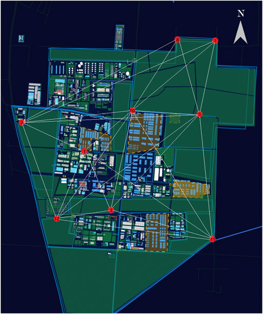
FIGURE 1. Monitoring station distribution in home-based care parks.

2.2 Data preprocessing

In the home-based care parks, each sensing device uploads the collected data to the database through the atmospheric monitoring gateway device using 4G or wired network, the process is shown in Figure 2, and the data upload frequency is 30 s.

FIGURE 2

FIGURE 2. Dataset construction process.

The data preprocessing in Figure 2 mainly has the following three steps, as shown in Figure 3.

(1) For missing values in the data, we fill in the values of the monitoring stations with the largest correlation coefficients.

(2) Due to network delay and other reasons, the time stamps of each atmospheric monitoring gateway device uploading data to the database are inconsistent. In order to keep the time stamps of the data of each monitoring station consistent, the data is resampled and the time interval is uniformly adjusted to 10 min, so as to ensure the regularity of the dataset. If the resampling time interval is too long, the inherent characteristics of the data will be lost, and if the resampling time interval is too short, there will be data redundancy, because the change trend of pollutant concentrations in a short period of time is not obvious.

(3) The data is normalized by the z-score method to speed up the training process. Its calculation formula is as follows:

$x^{\ast }=\frac{x-\overline{x}}{\sigma }(1)$

where $\overline{x}$ is the mean of the original data, $\sigma$ is the standard deviation of the original data, z-score is one of the most commonly used data normalization methods.

FIGURE 3

FIGURE 3. Data preprocessing.

The basic content of the preprocessed dataset is shown in Table 1.

TABLE 1

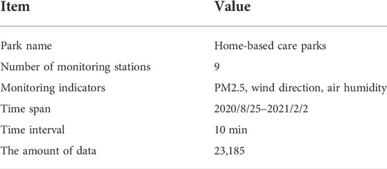
TABLE 1. Dataset.

2.3 Data analysis

In order to analyze the change rule of PM2.5 concentration, we visualized some PM2.5 concentration data, as shown in Figure 4. It can be seen from the figure that the highest concentration of PM2.5 occurs in the morning, and the concentration value gradually drops to the bottom in the afternoon, and gradually rises at night until the next morning, showing a periodic change. There is a strong correlation between different monitoring stations, and there are differences in the value.

FIGURE 4

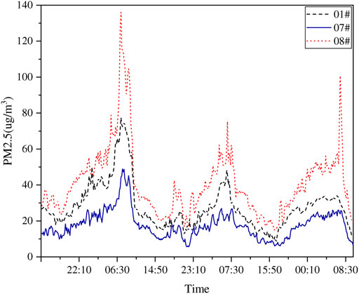
FIGURE 4. PM2.5 concentration change curve.

At a certain time, a certain pollution source produces PM2.5, which makes the indicators of surrounding monitoring stations larger. Under the influence of the wind field, the pollutants will spread along the wind direction, causing the indicators of downstream monitoring stations to increase, which leads to Spatial correlation of PM2.5. The temporal correlation can be explained in the time dimension, the PM2.5 concentration is high in the morning and the PM2.5 concentration is low in the afternoon, reflecting the periodicity of PM2.5. Therefore, PM2.5 is correlated in both time and space, and we need to capture this spatiotemporal correlation if we want to predict PM2.5.

Visualize the air humidity data, as shown in Figure 5. It can be seen from the figure that the change trend of air humidity is basically the same as that of PM2.5, both of which are cyclical, but the change trend of air humidity is ahead of PM2.5. When the air humidity reached the maximum value, PM2.5 did not reach the maximum value, but when the air humidity gradually decreased, PM2.5 showed an upward trend until the maximum value. This is because when the air humidity is too high, the water vapor content in the air increases, and the PM2.5 solid particles are surrounded by moisture. Due to the increase in moisture, the density of PM2.5 particles decreases and the concentration decreases, resulting in a decrease in the PM2.5 value. It can be seen from the above analysis that air humidity is indeed an important factor affecting PM2.5.

FIGURE 5

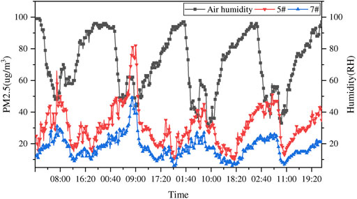
FIGURE 5. Air humidity and PM2.5 concentration change curve.

3 Model

In this subsection, according to the characteristics of home-based care parks, we first introduce the construction method of adjacency matrix, and then introduce our deep learning prediction model.

3.1 Adjacency matrix construction

In the home-based care park, we abstract the spatial distribution of N monitoring stations at a certain moment into a graph G = (V, E, A). Where V is a finite set of monitoring station sites; E is the edge set; A is the adjacency matrix of graph G.

Graphs can represent spatial associations between geospatial data, and when we predict PM2.5 concentrations, we need to consider the spatial associations between monitoring stations. In general, we use the straight-line distance between stations to represent the spatial association between stations. This value can be understood as the difficulty of interaction between stations. However, PM2.5 can diffuse completely freely and will be affected by wind. Therefore, in the home-based care parks scenario, we need to consider the effect of wind.

As we all know, the Gaussian diffusion model is the standard model to solve the problem of wind field diffusion. In order to obtain the influence of wind on the monitoring station, we introduce the Gaussian diffusion model. The basic formula of the model is as follows:

$C_0\left(x,y,z,u\right)=\frac{Q}{\pi u{\sigma }_{\text{y}}{\sigma }_{\text{z}}}\exp \left(-\frac{y^2}{2{\sigma }_{\text{y}}^2}-\frac{z^2}{2{\sigma }_{\text{z}}^2}\right)(2)$

where C₀ is the air pollutant concentration. x and y represent the downwind distance and the horizontal distance from the centerline of the wind direction, respectively. z represents the height of the pollution source. u is the horizontal wind speed. ${\sigma }_y$ and ${\sigma }_z$ represent the diffusion standard deviation in the horizontal and vertical directions, respectively. When only horizontal diffusion is considered, the formula can be simplified to Eq. 3 (Li et al., 2014), and the detailed calculation process is shown in Figure 6.

$cost\left(E_{ij}\right)=\left[F\left(D_i,D_M\right)+F\left(D_j,D_M\right)\right]\times L_{ij}(3)$

where i and j are the start and end points; $\mathit{cost}\left(E_{ij}\right)$ is used to describe the difficulty of diffusion of air pollutants from point i to point j; $E_{ij}$ is the edge between two points; $D_i$ and $D_j$ represent the wind direction azimuth of these two points; $D_M$ represents the azimuth of $E_{ij}$; $L_{ij}$ represents the length of $E_{ij}$, that is the distance between point i and point j; F represents a function that calculates the absolute value of the azimuth difference.

FIGURE 6

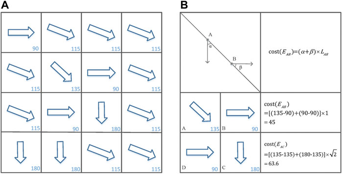
FIGURE 6. (A) Grid-based representation of a wind-field. (B) Computing the cost between adjacent cells.

Since the geographical space of the home-based care parks is not very large, the wind direction of each monitoring station at the same time can be regarded as the same, so the Eq. 3 can be simplified to Eq. 4, and the constant term can be omitted.

$cost\left(E_{ij}\right)=\left[2\times F\left(D_i,D_M\right)\right]\times L_{ij}(4)$

Based on the above analysis, we denote the elements $a_{ij}$ of the adjacency matrix as Eq. 5:

$a_{ij}=\{\begin{array}{l}\frac{1}{cost\left(E_{ij}\right)},i\ne j\\ 0,i=j\end{array}(5)$

where $\mathit{co}st\left(E_{ij}\right)$ represents the difficulty of diffusion of air pollutants from monitoring station i to j.

3.2 Proposed prediction model

We use $x_t^i$ to denote the PM2.5 concentration of node $i$ at time t, $X_t={\left(x_t^1,x_t^2,\dots ,x_t^N\right)}^{{\rm T}}\in {ℝ}^{N\times 1}$ represents the PM2.5 concentration of all nodes at time t, $\chi ={\left(X_1,X_2,\dots ,X_m\right)}^{{\rm T}}\in {ℝ}^{N\times 1\times m}$ represents the PM2.5 concentration value of all nodes in m time slices, ${\widehat{y}}^i=\left({\widehat{y}}_{m+1}^i,{\widehat{y}}_{m+2}^i,\dots ,{\widehat{y}}_{m+n}^i\right)$ represents the predicted value of node $i$ at n times in the future, $\widehat{Y}={\left({\widehat{y}}^1,{\widehat{y}}^2,\dots ,{\widehat{y}}^N\right)}^{{\rm T}}\in {ℝ}^{N\times n}$ represents the predicted value of all nodes at n times in the future, $Y={\left(y^1,y^2,\dots ,y^N\right)}^{{\rm T}}\in {ℝ}^{N\times n}$ represents the true value of all nodes n times in the future.

Figure 7 shows the overall framework of the STGODE-M model proposed in this paper. It consists of spatial-temporal graph ordinary differential equation networks module, external feature extraction module and output layer. The details of each part are as follows.

(1) Spatial-temporal graph ordinary differential equation networks module

FIGURE 7

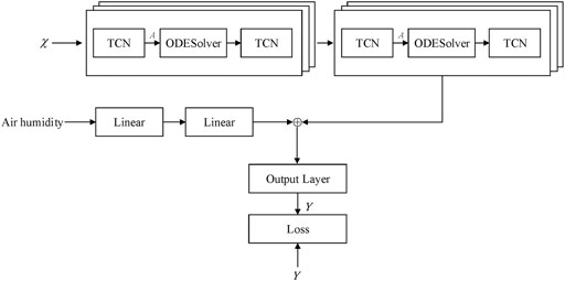
FIGURE 7. The framework of STGODE-M.

This module adopts the method of Fang et al. (2021) and their wording is reproduced in the method description section. GNNs update embeddings of nodes through aggregating features of their own and neighbors with a graph convolution operation. The classic form of convolution operation can be formulated as Eq. 6 and a discrete version is first shown as Eq. 7.

$H_{k+1}=GCN\left(H_k\right)=\sigma \left(\widehat{A}{H}_{k}W\right)(6)$

$H_{k+1}=H_k\times \widehat{A}\times U\times W+H_0(7)$

where $H_k$ denotes the input of the k-th graph convolutional layer, $\widehat{A}$ is the normalized adjacency matrix, and W is a learnable parameter matrix, which models the interaction among different features,$U$ is the temporal transform matrix, and $H_0$ denotes the initial input of GNN, which can be acquired through another neural network. However, such GNNs have been proved to suffer from over-smoothing problem when networks go deeper (Li et al., 2018b), which largely limits the capacity of modeling long-range dependencies. For this reason, we used STGODE block. The STGODE block adopts a three-layer structure, consisting of two temporal convolutional networks and one ODESolver. This structure can more fully capture the spatial-temporal information flow, and the stacked three-layer structure further enhances the ability of the model to mine the complex spatial-temporal correlations of PM2.5.

The STGODE network is an improvement of the ordinary graph convolutional network through the neural ordinary differential equation, so it can build a deeper network, and the model training has fewer parameters, so it has higher training efficiency. The formulas of the STGODE network are expressed as Eqs 8, 9:

$H\left(t\right)=ODESolve\left(\frac{dH\left(t\right)}{dt},H_0,t\right)(8)$

$\frac{dH\left(t\right)}{dt}=H\left(t\right)\times \left(\widehat{A}-I\right)+H\left(t\right)\times \left(U-I\right)+H\left(t\right)\times \left(W-I\right)+H_0(9)$

where U is the time transformation matrix, I is the identity matrix, H₀ represents the initial input, ODESolve is used as the Euler solver.

It is extremely important to find the approximate solution of the differential equation in the neural network, because in most cases it is difficult to find the function expression of the differential equation, or the expression is too complicated, in this case, the numerical calculation method can be used to find the approximate solutions to differential equations. Euler’s method is one of the simplest methods for finding approximate solutions of ordinary differential equations, and it is of great significance both for its numerical calculation ideas and for the solution of practical problems.

PM2.5 concentration is time-dependent, and how to fully capture this correlation is also very important. Most existing works use recurrent neural networks to capture temporal correlations, but these networks suffer from issues such as time-consuming iterations.

Temporal Convolutional Network (TCN) is a time-series convolutional neural network model proposed in 2018. It can be processed in parallel on a large scale, so the speed of the network will be faster during training and verification, and it can change the receptive field by increasing the number of layers, changing the expansion coefficient and the size of the filter, making the length of historical information more flexible, avoiding the problems of gradient dispersion and gradient explosion in RNN, and it takes less memory when training, especially for long sequences. To improve the model’s ability to model long-term temporal dependencies, we will use TCN. Its calculation process can be expressed as:

$H_{tcn}^l=\{\begin{array}{l}X,l=0\\ \sigma \left(W^l{\ast }_{d^l}{H}_{tcn}^{l-1}\right),l=\mathrm{1,2},\cdots ,L\end{array}(10)$

Where $\text{X}\in {\mathrm{ℝ}}^{N\times T\times F}$ is the input of the TCN, $H_{tcn}^l\in {\mathrm{ℝ}}^{N\times T\times F}$ is the output of the l-th layer TCN, W^l represents the l-th convolution kernel, $\text{σ}$ is the activation function. To expand the receptive field, we set the exponential dilation rate of temporal convolution as $d^l=2^{l-1}$. In the process, zero-padding strategy is utilized to keep time sequence length unchanged.

We represent this module abstractly as:

$O_h=f_1\left(\chi ;A\right)(11)$

where f₁ represents the STGODE module function, $\text{χ}$ represents the PM2.5 concentration data, A represents the adjacency matrix, and O_h represents the PM2.5 preliminary features extracted by the module.

(2) External feature extraction module

Fully connected neural network is one of the most common neural network models, which can map the data dimension to any dimension, and is often used as a simple feature extraction model. At the same time, the humidity of each monitoring station is the same, so the humidity data is one-dimensional data, and the feature extraction of one-dimensional data is more suitable for using a fully connected neural network. Fully connected neural networks are also used as feature extraction models in many deep learning papers. In this module, we introduce a fully connected neural network for embedding learning on air humidity data. The preliminary features of air humidity are expressed as O_other, and the processing is as follows:

$O_{other}=\sigma \left(w_{other}^2\sigma \left(w_{other}^1{m}_t+b_{other}^1\right)+b_{other}^2\right)(12)$

where w represents the weight matrix of the fully connected neural network, b represents the bias matrix of the fully connected neural network, $\text{σ}$ is the activation function, and m_t represents the air humidity at time t.

(3) Output layer

The above two preliminary features outputs are spliced according to the specified dimensions to perform feature fusion. The fusion of features here selects the splicing operation instead of simply adding different features, because the addition operation will mix different expressions into one variable, which is not conducive to the learning of feature differences. In this module, a max-pooling operation is first performed to selectively aggregate information from different blocks, and then a two-layer MLP is designed for feature mapping. We denote this module function as f₂, the above two preliminary feature outputs are spliced according to the specified dimensions, and the spliced feature vector O is obtained as shown in Eq. 13.

$O=O_h\oplus O_{other}(13)$

The final predicted value can be expressed as Eq. 14.

$\widehat{Y}=f_2\left(O\right)(14)$

4 Experiments

4.1 Experimental settings

We split the data set into training set, validation set and test set according to the ratio of 8:1:1, and use the historical data of the past day to predict the PM2.5 concentration in the next 10 min. The hidden dimensions of TCN blocks are set to 64, 32, 64, and 3 STGODE blocks are contained in each module, we set up two STGODE modules in total (Fang et al., 2021). We train our model using Adam optimizer with a learning rate of 0.001, the batch size is 128 and the training epoch is 100. We implemented the STGODE-M in the PyTorch framework (Paszke et al., 2019). Parameters of training model are also shown in Table 2.

TABLE 2

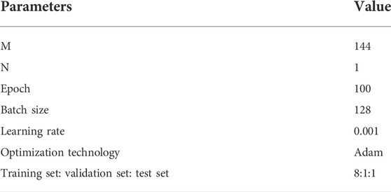
TABLE 2. Parameters of training model.

In order to measure the effectiveness of our proposed method, we use mean absolute errors (MAE), root mean squared errors (RMSE), mean absolute percentage errors (MAPE) and coefficient of determination (R2) as evaluation metrics. Their calculation process is explained by Eqs 15–18.

$\text{MAE}=\frac{1}{n}{\displaystyle \sum _{i=0}^n\left|{\widehat{y}}_i-y_i\right|}(15)$

$\text{RMSE}=\sqrt{\frac{1}{n}{\displaystyle \sum _{i=0}^n{\left({\widehat{y}}_i-y_i\right)}^2}}(16)$

$\text{MAPE}=\frac{100\%}{n}{\displaystyle \sum _{i=0}^n\left|\frac{\left({\widehat{y}}_i-y_i\right)}{y_i}\right|}(17)$

$R2=1-\frac{{\displaystyle \sum _{i=0}^n{\left({\widehat{y}}_i-y_i\right)}^2}}{{\displaystyle \sum _{i=0}^n{\left(\overline{y}-y_i\right)}^2}}(18)$

where $y_i$ represents the true value, ${\widehat{y}}_i$ represents the predicted value, $\overline{y}$ represents the variance, and n represents the number of samples.

RMSE is used to measure the deviation between the predicted value of the model and the true value, it is one of the most common evaluation indicators, the smaller the value, the better the model effect. MAE can better reflect the actual situation of the predicted value error, the smaller the MAE, the better the model effect. MAPE is 0 for a perfect model, greater than 100 for an inferior model. The range of R2 is [0, 1], and the larger the value, the stronger the fitting ability of the model.

4.2 Baselines

We selected 4 models from current work as our baseline models, the introduction of these models is as follows.

(1) LSTM (Krishan et al., 2019; Seng et al., 2021): LSTM model is a type of RNN designed to capture long term dependencies in sequential data. It is widely used in many time series forecasting problems and has achieved good results, but it cannot model spatial relationships.

(2) GRU (Becerra-Rico et al., 2020): GRU is a kind of recurrent neural network, and it is also proposed to solve the problems of long-term memory and gradient in backpropagation. However, GRU has fewer parameters, so training is faster or requires less data to generalize, but still cannot model spatial relationships.

(3) STGCN (Yu et al., 2018): The spatial-temporal graph convolutional network, which utilizes graph convolution and 1D convolution to capture spatial and temporal dependencies, respectively. It has achieved good results on traffic flow prediction, but it cannot simultaneously model spatial-temporal correlations and does not take into account the complex interactions between spatial and temporal dependencies. It has also been shown to have the problem of over-smoothing, unable to expand the spatial receptive field by increasing the depth, and the representations of all nodes will tend to be similar when the GCN stacks multiple layers.

(4) STAM-STGCN (Zeng et al., 2021): STAM-STGCN is a variant of STGCN. It can dynamically obtain the spatial-temporal correlation of data, but it has the same disadvantages as STGCN.

4.3 Results and analysis

In order to verify the effectiveness of the proposed adjacency matrix construction method, we compare the STGODE-M model using the proposed adjacency matrix construction method with the STGODE-M-OUT model using only distance-based adjacency matrix construction. The experimental results are shown in Table 3. It can be seen from the experimental results that the adjacency matrix construction method proposed in this paper is effective.

TABLE 3

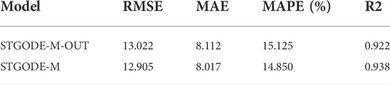
TABLE 3. Comparison of different adjacency matrices.

To verify the advantages of the proposed model, we choose four models in PM2.5 prediction as baselines, namely LSTM model, GRU model, STGCN model, and STAM-STGCN model. At the same time, in order to prove the auxiliary role of external features, we conducted ablation experiments to compare STGODE-M with external feature extraction module and STGODE model without external feature extraction module. Each model uses the same data set as the proposed method, and the experimental results are shown in Table 4. In order to more intuitively show the advantages of the proposed model, the results of each model evaluation index are displayed in the form of a bar chart, as shown in Figure 8.

TABLE 4

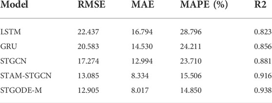
TABLE 4. Performance comparison of each model.

FIGURE 8

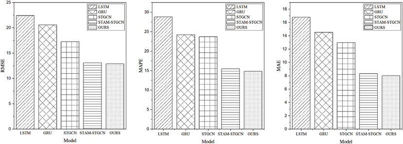
FIGURE 8. Performance metrics of each model.

As can be seen from the experimental data in Table 4, our model outperforms all baselines. Specifically, the PM2.5 concentration prediction effect of GRU is better than LSTM. Although both are variants of RNN, GRU has fewer parameters and is easier to converge. Further analysis, both GRU and LSTM are inferior to STGCN since they do not consider the spatial dependencies between monitoring stations. It can be seen that the STGCN model that can model the spatial-temporal dependence is better than the model that can only model the time dependence. STAM-STGCN is a variant of STGCN, which dynamically obtains the spatial-temporal correlation of data through the spatial-temporal attention mechanism, and has stronger predictive ability, but neither can model the spatial-temporal correlation at the same time, they do not take into account the complex interactions between spatial-temporal dependencies, and they all suffer from over-smoothing problems, which cannot expand the spatial receptive field by increasing depth. In addition, although STAM-STGCN has better prediction performance than STGCN, it has longer training time.

The number of monitoring stations in our experiment is limited, and thus the collected dataset is relatively small. During our experiments for the relatively small collected dataset, the performance tends to be stable when the number of STGODE block is set larger, resulting in a ‘basin effect’ of performance, which is that the performance can’t further improve with the increasing the number of STGODE block, but the complexity of the model will become much higher. We have tradeoff the performance and complexity simultaneously, and finally have choosen the number of STGODE block is 3, which is the most appropriate.

We compare the proposed model with existing deep learning methods for PM2.5 prediction, and the experimental results are shown in Table 5. It can be seen from the experimental results that our proposed model still has advantages.

TABLE 5

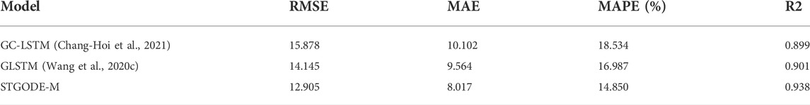
TABLE 5. Comparisons with the existing works about PM2.5 prediction with deep learning methods.

In addition, we compare STGODE-M with external feature extraction module and STGODE model without external feature extraction module. From the experimental results in Table 6, it can be seen that the STGODE model without external feature extraction module is slightly different. It is better than the baseline model, but inferior to the STGODE-M model with the addition of an external feature extraction module. Although the overall performance is not much different, it can also fully demonstrate that the external feature of air humidity does have an impact on PM2.5 concentration.

TABLE 6

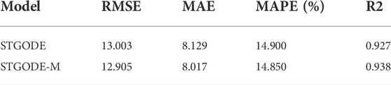
TABLE 6. Ablation experiment.

STGODE-M solves the problems of over-smoothing in STGCN model, and can expand the spatial receptive field by increasing the depth. However, our dataset has only 9 monitoring stations and the spatial relationship is relatively simple, so the effect of performance improvement is not very significant. In scenarios with more monitoring stations, the performance improvement effect will be more obvious. In future work, we will also collect relevant datasets for verification.

To compare the complexity of the models, we plot the training time comparison between the proposed model and the model with the best predictive ability among the baseline models, as shown in Figure 9. As can be seen from the figure, the proposed model has a faster training time, with an average training time of 63 s, while the average training time of the comparison model is 76 s, and the proposed model shortens the training time by 17.1%. NODE does not need to store all parameters while backpropagating, so it is more memory efficient and trains the model faster. NODE balances speed and accuracy through a discretization scheme, and makes it different during training and inference, so it has the advantage of adaptive computing. The training efficiency of the STGODE-M model has obvious advantages, which are attributed to the characteristics of low memory consumption, high adaptive computing power and short training time of neural ordinary differential equation (Chen et al., 2018b; Poli et al., 2019).

FIGURE 9

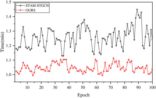
FIGURE 9. Model training time comparison.

To further compare the predictive power of each model, we plotted each model’s predicted versus true value on the test set, as shown in Figure 10. As can be seen from the figure, our model exhibits the best fit between the predicted and true values, followed by STAM-STGCN, while the STGCN model has the worst fit.

FIGURE 10

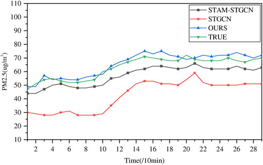
FIGURE 10. The comparison of prediction results between our model and other models.

5 Conclusion

PM2.5 has a serious impact on people’s brain and respiratory system. However, because of high blood pressure, poor resistance, and weak awareness of prevention, the elderly have become the primary danger targets. Therefore, accurate prediction of PM2.5 is of great significance to the health of the elderly.

At this stage, there has been a lot of work to solve complex spatial-temporal prediction problems, but few people have uniformly modeled spatial-temporal dependencies, and little attention has been paid to how to extract long-term dependencies without being affected by over-smoothing problems, the factor of air humidity is also easily overlooked. Based on this, this paper uses a new tensor-based spatial-temporal prediction model STGODE-M, and uses air humidity as an auxiliary feature to fuse air humidity features through an external feature fusion strategy to further improve PM2.5 prediction precision. Experiments are conducted on a real home-based care parks atmospheric dataset, and the experimental results show that STGODE-M improves the RMSE performance by about 1.3%, the MAE performance by 3.8%, the MAPE performance by 4.2%, and the model training efficiency by 17.1% compared with the optimal baseline. Therefore, the proposed model can provide better guarantee for the healthy travel of the elderly.

Data availability statement

The raw data supporting the conclusion of this article will be made available by the authors, without undue reservation.

Author contributions

QZ performed conceptualization, methodology, design, formal analysis, reviewing, and editing. CW carried out conceptualization, methodology, design, investigation, data collection, data analysis, and writing original draft preparation. GC done conceptualization, methodology, formal analysis, reviewing, and editing. HD involved in data curation, critical analysis, writing, reviewing, and editing. SW contributed in formal analysis, reviewing, and editing. All authors contributed to the article and approved the submitted version.

Funding

This work was supported by the National Natural Science Foundation of China under Grant No. 61701284, the Innovative Research Foundation of Qingdao under Grant No. 19-6-2-1-cg, the Elite Plan Project of Shandong University of Science and Technology under Grant Nos. skr21-3-B-048, the Sci. & Tech. Development Fund of Shandong Province of China under Grant Nos. ZR202102230289, ZR202102250695 and ZR2019LZH001, the Humanities and Social Science Research Project of the Ministry of Education under Grant No. 18YJAZH017, the Taishan Scholar Program of Shandong Province, the Shandong Chongqing Science and Technology Cooperation Project under Grant No. cstc2020jscx-lyjsAX0008, the Sci. & Tech. Development Fund of Qingdao under Grant No. 21-1-5-zlyj-1-zc, SDUST Research Fund under Grant No. 2015TDJH102, and the Science and Technology Support Plan of Youth Innovation Team of Shandong higher School under Grant No. 2019KJN024.

Acknowledgments

The authors would like to extend their gratitude to the reviewers and the editors for their valuable and constructive comments, which have greatly improved the quality of this paper.

Conflict of interest

The authors declare that the research was conducted in the absence of any commercial or financial relationships that could be construed as a potential conflict of interest.

Publisher’s note

All claims expressed in this article are solely those of the authors and do not necessarily represent those of their affiliated organizations, or those of the publisher, the editors and the reviewers. Any product that may be evaluated in this article, or claim that may be made by its manufacturer, is not guaranteed or endorsed by the publisher.

References

Amato, F., Guignard, F., Robert, S., and Kanevski, M. (2020). A novel framework for spatio-temporal prediction of environmental data using deep learning. Sci. Rep. 10 (1), 1–11. doi:10.1038/s41598-020-79148-7

PubMed Abstract | CrossRef Full Text | Google Scholar

Becerra-Rico, J., Aceves-Fern´andez, M. A., Esquivel-Escalante, K., and Pedraza-Ortega, J. C. (2020). Airborne particle pollution predictive model using gated recurrent unit (gru) deep neural networks. Earth Sci. Inf. 13, 821–834. doi:10.1007/s12145-020-00462-9

CrossRef Full Text | Google Scholar

Chang-Hoi, H., Park, I., Oh, H. R., Gim, H. J., Hur, S. K., Kim, J., et al. (2021). Development of a PM2.5 prediction model using a recurrent neural network algorithm for the Seoul metropolitan area, Republic of Korea. Atmos. Environ. 245, 118021. doi:10.1016/j.atmosenv.2020.118021

CrossRef Full Text | Google Scholar

Chen, L., Yang, D., Zhang, D., Wang, C., Li, J., and Nguyen, T. M. T. (2018). Deep mobile traffic forecast and complementary base station clustering for c-ran optimization. J. Netw. Comput. Appl. 121, 59–69. doi:10.1016/j.jnca.2018.07.015

CrossRef Full Text | Google Scholar

Chen, R. T. Q., Rubanova, Y., Bettencourt, J., and Duvenaud, D. (2018). “Neural ordinary differential equations[J] in Paper presented at 31nd Conference on Neural Information Processing Systems (NeurIPS 2018), Montréal, Canada, Decemcer, 2018, 1–13.

Google Scholar

Chen, B., Song, Z., Pan, F., and Huang, Y. (2022). Obtaining vertical distribution of pm2.5 from caliop data and machine learning algorithms. Sci. Total Environ. 805, 150338. doi:10.1016/j.scitotenv.2021.150338

PubMed Abstract | CrossRef Full Text | Google Scholar

Chen, Y. C., and Li, D. C. (2021). Selection of key features for PM2.5 prediction using a wavelet model and RBF-LSTM. Appl. Intell. (Dordr). 51 (4), 2534–2555. doi:10.1007/s10489-020-02031-5

CrossRef Full Text | Google Scholar

Cui, Z., Henrickson, K., Ke, R., and Wang, Y. (2019). Traffic graph convolutional recurrent neural network: A deep learning framework for network-scale traffic learning and forecasting. IEEE Trans. Intell. Transp. Syst. 21 (11), 4883–4894. doi:10.1109/TITS.2019.2950416

CrossRef Full Text | Google Scholar

Dai, H., Huang, G., Zeng, H., and Yang, F. (2021). PM2.5 concentration prediction based on spatiotemporal feature selection using XGBoost-MSCNN-GA-LSTM. Sustainability 13 (21), 12071. doi:10.3390/su132112071

CrossRef Full Text | Google Scholar

Fang, Z., Long, Q., Song, G., and Xie, K. (2021). “Spatial-temporal graph ode networks for traffic flow forecasting,” in Paper presented at the 27th ACM SIGKDD Conference on Knowledge Discovery and Data Mining, August 2021.

Google Scholar

Feng, J., Chen, X., Gao, R., Zeng, M., and Li, Y. (2018). Deeptp: An end-to-end neural network for mobile cellular traffic prediction. IEEE Netw. 32 (6), 108–115. doi:10.1109/MNET.2018.1800127

CrossRef Full Text | Google Scholar

Gao, X., and Li, W. (2021). A graph-based LSTM model for PM2.5 forecasting. Atmos. Pollut. Res. 12 (9), 101150. doi:10.1016/j.apr.2021.101150

CrossRef Full Text | Google Scholar

Guo, S., Lin, Y., Feng, N., Song, C., and Wan, H. (2019). Attention based spatial-temporal graph convolutional networks for traffic flow forecasting. Pap. Present. A. T. 33rd AAAI Conf. Artif. Intell. 33, 922–929. doi:10.1609/aaai.v33i01.3301922

CrossRef Full Text | Google Scholar

Huang, M., Zhang, T., Wang, J., and Zhu, L. (2015). “A new air quality forecasting model using data mining and artificial neural network,” in Proceeding of the 2015 6th IEEE International Conference on Software Engineering and Service Science (ICSESS), Beijing, China, September 2015 (IEEE), 259–262.

CrossRef Full Text | Google Scholar

Jeong, S.-G., Kim, M., Lee, T., and Lee, J. (2021). Application of pre-filter system for reducing indoor pm2.5 concentrations under different relative humidity levels. Build. Environ. 192, 107631. doi:10.1016/j.buildenv.2021.107631

CrossRef Full Text | Google Scholar

Krishan, M., Jha, S., Das, J., Singh, A., Goyal, M. K., and Sekar, C. (2019). Air quality modelling using long short-term memory (lstm) over nct-Delhi, India. Air Qual. Atmos. Health 12 (8), 899–908. doi:10.1007/s11869-019-00696-7

CrossRef Full Text | Google Scholar

Li, L., Gong, J., and Zhou, J. (2014). Spatial interpolation of fine particulate matter concentrations using the shortest wind-field path distance. PloS one 9, e96111. doi:10.1371/journal.pone.0096111

PubMed Abstract | CrossRef Full Text | Google Scholar

Li, Y., Yu, R., Shahabi, C., and Liu, Y. (2018). “Diffusion convolutional recurrent neural network: Data-driven traffic forecasting,” in Paper presented at the 6th International Conference on Learning Representations, April 2018.

Google Scholar

Li, Q., Han, Z., and Wu, X.-M. (2018). “Deeper insights into graph convolutional networks for semi-supervised learning,” in Thirty-second AAAI conference on artificial intelligence.

CrossRef Full Text | Google Scholar

Li, Y., Wang, J., Sun, X., Li, Z., Liu, M., and Gui, G. (2020). Smoothing-aided support vector machine based nonstationary video traffic prediction towards b5g networks. IEEE Trans. Veh. Technol. 69 (7), 7493–7502. doi:10.1109/TVT.2020.2993262

CrossRef Full Text | Google Scholar

Li, T., Hua, M., and Wu, X. (2020). A hybrid cnn-lstm model for forecasting particulate matter (pm2.5). Ieee Access 8, 26933–26940. doi:10.1109/ACCESS.2020.2971348

CrossRef Full Text | Google Scholar

Pak, U., Ma, J., Ryu, U., Ryom, K., Juhyok, U., Pak, K., et al. (2020). Deep learning-based PM2.5 prediction considering the spatiotemporal correlations: A case study of beijing, China. Sci. Total Environ. 699, 133561. doi:10.1016/j.scitotenv.2019.07.367

PubMed Abstract | CrossRef Full Text | Google Scholar

Paszke, A., Gross, S., Massa, F., Lerer, A., Bradbury, J., Chanan, G., et al. (2019). “Pytorch: An imperative style, high-performance deep learning library,” in Advances in neural information processing systems, 32.

Google Scholar

Poli, M., Massaroli, S., Park, J., Yamashita, A., Asama, H., and Park, J., Graph neural ordinary differential equations[J]. arXiv preprint arXiv:1911.07532, 2019.

Google Scholar

Puett, R. C., Poulsen, A. H., Taj, T., Ketzel, M., Geels, C., Brandt, J., et al. (2020). Relationship of leukaemias with long-term ambient air pollution exposures in the adult Danish population. Br. J. Cancer 123 (12), 1818–1824. doi:10.1038/s41416-020-01058-2

PubMed Abstract | CrossRef Full Text | Google Scholar

Qi, Y., Li, Q., Karimian, H., and Liu, D. (2019). A hybrid model for spatiotemporal forecasting of PM2.5 based on graph convolutional neural network and long short-term memory. Sci. Total Environ. 664, 1–10. doi:10.1016/j.scitotenv.2019.01.333

PubMed Abstract | CrossRef Full Text | Google Scholar

Seng, D., Zhang, Q., Zhang, X., Chen, G., and Chen, X. (2021). Spatiotemporal prediction of air quality based on LSTM neural network. Alexandria Eng. J. 60, 2021–2032. doi:10.1016/j.aej.2020.12.009

CrossRef Full Text | Google Scholar

Tian, Y., Liu, X., Huo, R., Shi, Z., Sun, Y., Feng, Y., et al. (2021). Organic compound source profiles of pm2.5 from traffic emissions, coal combustion, industrial processes and dust. Chemosphere 278, 130429. doi:10.1016/j.chemosphere.2021.130429

PubMed Abstract | CrossRef Full Text | Google Scholar

Tong, W., Li, L., Zhou, X., Hamilton, A., and Zhang, K. (2019). Deep learning pm2.5 concentrations with bidirectional lstm rnn. Air Qual. Atmos. Health 12 (4), 411–423. doi:10.1007/s11869-018-0647-4

CrossRef Full Text | Google Scholar

Wang, P., Zhang, H., Qin, Z., and Zhang, G. (2017). A novel hybrid-Garch model based on ARIMA and SVM for PM 2.5 concentrations forecasting. Atmos. Pollut. Res. 8 (5), 850–860. doi:10.1016/j.apr.2017.01.003

CrossRef Full Text | Google Scholar

Wang, X., Zhang, R., and Yu, W. (2019). The effects of pm2.5 concentrations and relative humidity on atmospheric visibility in beijing. J. Geophys. Res. Atmos. 124 (4), 2235–2259. doi:10.1029/2018JD029269

CrossRef Full Text | Google Scholar

Wang, Y., Wang, H., and Zhang, S. (2020). Prediction of daily pm2.5 concentration in China using data-driven ordinary differential equations. Appl. Math. Comput. 375, 125088. doi:10.1016/j.amc.2020.125088

CrossRef Full Text | Google Scholar

Wang, Y., Wang, D., and Tang, Y. (2020). Clustered hybrid wind power prediction model based on arma, pso-svm, and clustering methods. IEEE Access 8, 17071–17079. doi:10.1109/ACCESS.2020.2968390

CrossRef Full Text | Google Scholar

Wang, S., Li, Y., Zhang, J., Meng, Q., Meng, L., and Gao, F. (2020). “Pm2.5-gnn: A domain knowledge enhanced graph neural network for pm2.5 forecasting[C],” in Proceedings of the 28th International Conference on Advances in Geographic Information Systems, 163–166.

Google Scholar

Wu, Z., Pan, S., Chen, F., Long, G., Zhang, C., and Yu, P. S. (2020). A comprehensive survey on graph neural networks. IEEE Trans. Neural Netw. Learn. Syst. 32, 4–24. doi:10.1109/TNNLS.2020.2978386

CrossRef Full Text | Google Scholar

Xiao, X., Duan, H., and Wen, J. (2020). A novel car-following inertia gray model and its application in forecasting short-term traffic flow. Appl. Math. Model. 87, 546–570. doi:10.1016/j.apm.2020.06.020

CrossRef Full Text | Google Scholar

Xiao, F., Yang, M., Fan, H., Fan, G., and Al-qaness, M. A. (2020). An improved deep learning model for predicting daily PM2.5 concentration[J]. Sci. Rep. 10 (1), 1–11. doi:10.1038/s41598-020-77757-w

PubMed Abstract | CrossRef Full Text | Google Scholar

Xiao, Q., Geng, G., Cheng, J., Liang, F., Li, R., Meng, X., et al. (2021). Evaluation of gap-filling approaches in satellite-based daily PM2.5 prediction models. Atmos. Environ. 244, 117921. doi:10.1016/j.atmosenv.2020.117921

CrossRef Full Text | Google Scholar

Xu, M., Yang, Y., Han, M., Qiu, T., and Lin, H. (2018). Spatio-temporal interpolated echo state network for meteorological series prediction. IEEE Trans. Neural Netw. Learn. Syst. 30, 1621–1634. doi:10.1109/TNNLS.2018.2869131

PubMed Abstract | CrossRef Full Text | Google Scholar

Yu, B., Yin, H., and Zhu, Z. (2018). “Spatio-temporal graph convolutional networks: A deep learning framework for traffic forecasting,” in Paper presented at the 27th International Joint Conference on Artificial Intelligence, July 2018, 3634–3640.

CrossRef Full Text | Google Scholar

Yue, H., He, C., Huang, Q., Yin, D., and Bryan, B. A. (2020). Stronger policy required to substantially reduce deaths from pm2.5 pollution in China. Nat. Commun. 11, 1–10. doi:10.1038/s41467-020-15319-4

PubMed Abstract | CrossRef Full Text | Google Scholar

Zeng, Q., Sun, Q., Chen, G., Duan, H., Li, C., and Song, G. (2020). Traffic prediction of wireless cellular networks based on deep transfer learning and cross-domain data. IEEE Access 8, 172387–172397. doi:10.1109/ACCESS.2020.3025210

CrossRef Full Text | Google Scholar

Zeng, Q., Wang, C., Chen, G., and Duan, H. (2021). PM2.5 concentration forecasting in industrial parks based on attention mechanism spatiotemporal graph convolutional networks. Wirel. Commun. Mob. Comput., 1–10. doi:10.1155/2021/7000986

CrossRef Full Text | Google Scholar

Zhang, C., Zhang, H., Yuan, D., and Zhang, M. (2018). Citywide cellular traffic prediction based on densely connected convolutional neural networks. IEEE Commun. Lett. 22, 1656–1659. doi:10.1109/LCOMM.2018.2841832

CrossRef Full Text | Google Scholar

Zhang, C., Zhang, H., Qiao, J., Yuan, D., and Zhang, M. (2019). Deep transfer learning for intelligent cellular traffic prediction based on cross-domain big data. IEEE J. Sel. Areas Commun. 37, 1389–1401. doi:10.1109/JSAC.2019.2904363

CrossRef Full Text | Google Scholar

Zhao, L., Song, Y., Zhang, C., Liu, Y., Wang, P., Lin, T., et al. (2019). T-Gcn: A temporal graph convolutional network for traffic prediction. IEEE Trans. Intell. Transp. Syst. 21, 3848–3858. doi:10.1109/TITS.2019.2935152

CrossRef Full Text | Google Scholar

Zhao, C., Wang, Q., Ban, J., Liu, Z., Zhang, Y., Ma, R., et al. (2020). Estimating the daily PM2.5 concentration in the Beijing-Tianjin-Hebei region using a random forest model with a 0.01° × 0.01° spatial resolution. Environ. Int. 134, 105297. doi:10.1016/j.envint.2019.105297

PubMed Abstract | CrossRef Full Text | Google Scholar

Zhou, H., Zhang, F., Du, Z., and Liu, R. (2021). Forecasting pm2.5 using hybrid graph convolution-based model considering dynamic wind-field to offer the benefit of spatial interpretability. Environ. Pollut. 273, 116473. doi:10.1016/j.envpol.2021.116473

PubMed Abstract | CrossRef Full Text | Google Scholar

Zhu, H., and Lu, X. (2016). “The prediction of PM2.5 value based on ARMA and improved BP neural network model[C],” in Proceeding of the 2016 International Conference on Intelligent Networking and Collaborative Systems (INCoS), Ostrava, Czech Republic, September 2016 (IEEE), 515–517.

Google Scholar