 Dusan Jandacka
 Daniela Durcanska1
 Robert Cibula
- 1Department of Highway and Environmental Engineering, Faculty of Civil Engineering, University of Žilina, Žilina, Slovakia
- 2Research Centre, University of Žilina, Žilina, Slovakia
Particulate matter (PM) is present in the surrounding air. The tunnel environment is no exception, where the PM source is road traffic. In a broader sense, the tunnel can be described as a separate point source of air pollution from which PM pollutants spread to the portal parts and the external environment. PM originates from the exhaust and non-exhaust processes of road traffic (brake wear, tire wear, road surface wear, and road dust re-suspension). This study deals with the specification of non-exhaust PM emissions in a tunnel environment where the primary source is road traffic. PM measurements took place in the “Považský Chlmec” highway tunnel with a length of 2,118 m directly in the tunnel tube and near the tunnel portal. PM measurements were performed using gravimetric and optical methods. PM chemical analyses were performed using energy-dispersive X-ray fluorescence (EDXRF). The concentration of PM in the tunnel was on average: PM10 = 30.76 μg/m3 and PM2.5 = 15.66 μg/m3 and near the tunnel portal PM10 = 14.38 μg/m3 and PM2.5 = 8.74 μg/m3. The average traffic volume in the tunnel tube was 2,274 veh/24 h. Using EDXRF, the main chemical elements Al, Br, Ca, Cl, Cr, Cu, Fe, K, Mg, Mn, Na, P, Si, S, Ti, and Zn were identified in the PM. Chemical element concentrations in PM10 and PM2.5 were subjected to factor analysis (FA) and principal component analysis (PCA) to determine the origin of PM. Two sources were identified for PM10 and three for PM2.5. Absolute principal component scores (APCS) in conjunction with multiple regression analysis (MRA) were used to determine the source contribution to the production of PM10 and PM2.5.
1 Introduction
PM emissions from road traffic come from two primary sources: exhaust processes and degradation of vehicle parts and road surfaces. The latter, which includes all airborne particulate emissions generated by vehicles, road wear, and road dust re-suspension, is defined as PM emissions—non-exhaust emissions. The share of PM emissions from non-exhaust sources has increased rapidly in recent years owing to a significant reduction in combustion emissions and currently accounts for approximately 90 % of all PM emissions from road traffic (Rexeis and Hausberger, 2009; Timmers and Achten, 2016; OECD, 2020). Particles from non-exhaust processes that have settled on the road surface can also be re-suspended by road traffic turbulence (US-EPA, 2011; de la Paz et al., 2015). Non-exhaust PM emissions can be divided into direct emissions from wear (brake wear, tire wear, and road wear) and road dust re-suspension. PM from non-exhaust processes is a major component of the PM2.5-10 coarse fraction (Fenger et al., 1998; OECD, 2020; Harrison et al., 2021).
Any combustion process leads to the formation of substances that enter the ambient air but are not kept in their original state. High saturation then occurs during cooling. The homogeneous nuclear form of the particles (several nanometers) usually coagulates rapidly into larger particles, and the number of particles is reduced. Particles with sizes between 50 nm and 1 µm are emitted by transport; however, nanoparticles are also emitted in large numbers. The particles emitted from vehicle engines include organic and inorganic particles and soot. Organic particles are mainly the result of the imperfect combustion of fuel or lubricating oils. Emissions from petrol engines are mainly characterized by high concentrations of fine particles. Soot formation is associated with the operation of diesel cars, especially heavy trucks. During the combustion of fuels, SO2 and NOx gases are produced, which can transform (condense) into sulfates and nitrates and form particles in the air. PM exhaust emissions may include Al, Cd, Cu, Fe, Mg, Ni, Pb, Zn, and K (Agarwal, 2007; Liati et al., 2012; Pant and Harrison, 2013; Reşitoʇlu et al., 2015; Filonchyk et al., 2018; Chernyshev et al., 2019; Hao et al., 2019; Yang et al., 2019).
Tire wear is the largest source of PM10. However, not all tire abrasion particles enter the air but are deposited near roads. Chemical analysis showed that the tire material contains different types of rubber and a relatively large amount of Zn and other metals (such as Ca, Fe, and Pd). Primary carbon, organic carbon, polycyclic aromatic hydrocarbons, and metals (such as Zn, S, Si, Ca, and Fe) were present in the abrasion particles (Hildemann et al., 1991; Legret and Pagotto, 1999; Kennedy and Gadd, 2000; Yli-Tuomi et al., 2005; Thorpe and Harrison, 2008; Gustafsson, 2018; OECD, 2020; Harrison et al., 2021).
The PM formed during brake lining abrasion contained a larger amount of fine particles than would correspond to the formation of particles during the mechanical process. PM2.5 has the largest share in PM10, up to 70 %. The particles produced during brake lining abrasion contain many different metals (such as Fe, Cu, Ca, Zn, Pb, Mo, Mn, and Al), polyaromatic hydrocarbons, inorganic components (such as Si, Ba, Fe, Mg, P, and Cl), and elemental carbon (Hildemann et al., 1991; Legret and Pagotto, 1999; Kennedy and Gadd, 2000; Yli-Tuomi et al., 2005; Thorpe and Harrison, 2008; OECD, 2020; Harrison et al., 2021).
Road wear emissions are much more difficult to quantify on their own than tire and brake abrasion emissions. This is partly due to the complexity of the asphalt mixture composition (Leitner et al., 2019; Kováč et al., 2021; Briliak and Remišová, 2022; Briliak and Remišová, 2022) and partly because particles from the abrasion are challenging to distinguish from particles of the re-suspended material. Asphalt pavements mainly contain organic compounds. Some metals such as V, Ni, Fe, Mg, Ca, and Si are also present in asphalt pavement layer samples (Yli-Tuomi et al., 2005; Thorpe and Harrison, 2008; Gustafsson, 2018; OECD, 2020; Harrison et al., 2021; Jandacka et al., 2021).
The origin of PM from road surface abrasion was also investigated in the authors’ workplaces, along with the grinding of various asphalt mixtures under laboratory conditions. Various chemical elements have been identified in asphalt mixtures and PM. The most important ones are Ca, Si, and S. Ca and Si originate from different types of aggregates and S from the asphalt binder (Jandacka et al., 2021).
Road dust re-suspension includes all particles deposited on the road surface after their formation (from tire wear, brakes, road surfaces, and other car parts). For TSP, the share of emissions from abrasion was significantly higher than the share of exhaust emissions. As the share of PM in exhaust emissions has decreased significantly in recent years, non-exhaust PM emissions have begun to exceed those in PM (Bilos et al., 2001; Thorpe and Harrison, 2008; de la Paz et al., 2015; Fullova et al., 2016; Alves et al., 2018; OECD, 2020; Harrison et al., 2021).
Surrounding PM are chemically non-specific pollutants from various sources that appear to determine their toxicological properties in accordance with their chemical composition, size, and solubility. PM10 and PM2.5, including inhalable particles, are small enough to penetrate the thoracic region of the respiratory system. The effects of respirable PM result from short-term exposure (hours, days) and long-term exposure (months, years), including respiratory and cardiovascular morbidities, such as worsening asthma, respiratory tract, increasing hospitalizations, mortality from cardiovascular and respiratory diseases, and lung cancer (Pope, 2002; WHO, 2007; Beelen et al., 2008; Samoli et al., 2008; Health Organization, 2013; Morabito et al., 2020).
As part of our research, measurements of PM10 and PM2.5 were taken in a tunnel environment. The measurements were taken simultaneously in two places: inside the tunnel and outside near the tunnel portal. The measurements were performed under strict safety measures, as it was necessary to ensure that the measurements in the tunnel tube were during the uninterrupted operation of the tunnel. The measurements were planned such that the first measurement period was performed before the standard maintenance of the tunnel, and the second measurement period was subsequently performed. The aim of this distribution of measurements was to determine the importance of tunnel cleaning from the perspective of tunnel environment pollution by PM. Another goal was to map the PM concentration in the tunnel environment—inside the tunnel and outside near the tunnel portal. The primary source of air pollution PM is road traffic, which generates PM from the exhaust and non-exhaust processes. Subsequently, the PM concentrations measured inside the tunnel were compared with the PM concentrations outside near the tunnel portal to determine the dispersion of PM to the outside environment. The PM samples were subjected to chemical analyses to determine the inorganic composition. Knowledge about the chemical composition of PM is mainly used to identify PM sources. For these purposes, multidimensional statistical methods, including PCA and FA, have been used with great popularity and success. (Manta et al., 2002; Guo et al., 2004; Song et al., 2006; Lu et al., 2010; Yang et al., 2011; Jandacka et al., 2017; Jain et al., 2018). Our goal was to determine the internal interconnections of individually analyzed chemical elements (mutual correlations), which led to the creation of specific groups of elements interconnected by their origins, that is, potential sources. The tunnel environment is an ideal place to determine the share of individual PM sources from road traffic; that is, exhaust emissions of PM or non-exhaust emissions of PM (brake wear, tire wear, road wear, and re-suspension). To implement this plan, it is necessary to have information on the origin of the chemical elements, that is, from which road traffic parts can come. This has been addressed by several studies that have investigated the composition of PMs in simulations or by in situ measurements (Yli-Tuomi et al., 2005; Thorpe and Harrison, 2008; Reşitoʇlu et al., 2015; Filonchyk et al., 2018; Chernyshev et al., 2019; Hao et al., 2019; Yang et al., 2019; Morabito et al., 2020; OECD, 2020; Celo et al., 2021; Harrison et al., 2021; Jandacka and Durcanska, 2021). In the process of investigating the chemical composition of PM, chemical elements were discovered that correspond to the studies already carried out (Allen et al., 2001; Gillies et al., 2001; Handler et al., 2008; He et al., 2008; Chellam et al., 2011; Brito et al., 2013; Cui et al., 2016; Hao et al., 2019).
On the one hand, the introduction of electric vehicles reduces exhaust emissions, but on the other hand, with increasing vehicle weight and the number of cars, non-exhaust PM emissions increase (OECD, 2020). Therefore, monitoring the production of PM from road traffic, particularly the share of non-exhaust PM emissions, is necessary. The research presented in this article contributes to raising awareness regarding PM emissions from road traffic.
2 Materials and methods
2.1 Measurement location
PM measurements were taken in a tunnel environment, inside the tunnel, and near the tunnel portal (western portal) in the city of Žilina, Považský Chlmec Tunnel. The measurement in the tunnel tube was performed in the second parking bay in the direction of the eastern portal (Figure 1).
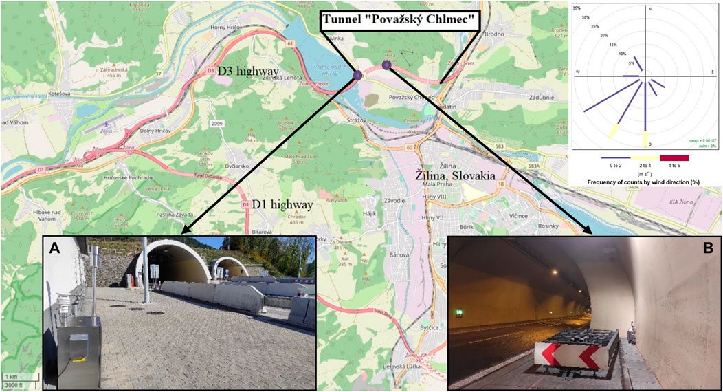
FIGURE 1. Measurement location—tunnel Považský Chlmec, Žilina, Slovakia. (A) Measuring station outside, near the tunnel portal 49°14′43.1″N, 18°42′27.2″E. (B) Measuring station inside the tunnel 49°14′51.9″N, 18°42′56.8″E) and wind rose (map source: © OpenStreetMap contributors).
The Považský Chlmec tunnel is a two-pipe highway tunnel in Slovakia that measures 2,218 m. It is located northwest of the center of Žilina and is part of the D3 highway section Žilina, Strážov—Žilina, and Brodno. The tunnel is part of the D3 highway, which belongs to multimodal corridor no. VI and the Trans-European Highway in the north–south direction, the purpose of which is to transfer transit passenger and freight traffic through Slovakia. The category 2T-8 tunnel with a road width between curbs of 8 m and a cross-sectional height of 4.8 m according to STN 737507 consists of two tunnel tubes, each of which has two lanes in one direction. In terms of safety, the tunnel has two parking bays and eight transverse connections (Širilla and Schmidt, 2017).
PM measurements were performed to determine the concentrations of PM10 and PM2.5 directly in the tunnel tube (PM2.5_IN, PM10_IN) and the portal part (PM2.5_OUT, PM10_OUT) and their elemental chemical composition (presence of chemical elements in PM). PM measurements were taken during two periods: before tunnel maintenance (1–7 October, 2020) and after tunnel maintenance (12–20 October, 2020). Measurements were taken across a total of 16 days.
2.2 Particulate matter measurement
Two methods were used to measure PM10 and PM2.5: the reference gravimetric (4x Leckel LVS3 devices) and optical methods (Fidas 200S and APM-2). 2x Leckel devices and an APM-2 device were used inside the tunnel. 2x Leckel devices and a Fidas 200S device were used near the tunnel portal.
A reference method (gravimetric method) was applied according to the STN EN 12341 standard (2016) to establish the amount of ambient PM in the air. Sampling was performed using three low-volume flow samplers (LECKEL LVS3, Sven Leckel Ingenieurbüro GmbH). Two PM fractions were monitored concurrently: PM10 and PM2.5. PM was collected on nitrocellulose filters for 24 h (12 a.m.–12 a.m. the next day). Finally, using this method, we obtained 16 samples corresponding to 24-h sampling for each PM fraction inside the tunnel and at the tunnel portal (32 filters for each PM fraction—in sum, 64 exposed filters). The nanocellulose filters had a diameter of 47 mm, and the PM was collected at a fixed air flow rate of 2.3 m3/h, after which, the mass of PM collected on the filters was determined using microbalances, calculated based on the known volume of air obtained during sampling (µg/m3). The PM2.5-10 concentration was determined as the difference between PM10 and PM2.5. All exposed filters (PM samples) were used for the elemental chemical analysis. All necessary steps, including weighing, were taken to ensure the quality of the samples and PM concentrations. We calibrated all of the measuring instruments as prescribed by the STN EN 12341 standard. We quantified the total uncertainty of the method for PM2.5, and PM10, consisting of partial uncertainties—the sampling of PM by a flow pump and weighing of clean and exposed nitrocellulose filters. This method was maintained as accredited in the workplace.
A Fidas 200S optical measurement device was also used to continuously measure PM concentrations near the tunnel portal. Fidas 200S utilizes the acknowledged principle of single-particle light-scattering size analysis and is equipped with a high-intensity LED light source (dp, min = 180 nm). The sampling system of the Fidas® 200S was operated with a volume flow of approximately 0.3 m3/h. The actual aerosol sensor is an optical aerosol spectrometer that determines the particle size using Lorenz–Mie scattered light analysis of single particles. Although the optical measurement technique determines the particle mass indirectly (equivalence method), the empirical knowledge used in processing the measured data ensures an excellent correlation with the standard reference method. We ensured the quality of the measured data using the Fidas 200S instrument by comparing the measurements with the reference gravimetric method (accredited test for measuring PM10 and PM2.5 in ambient air). The comparison measurements showed a high correlation coefficient between the measured concentrations of PM10 r = 0.93 and PM2.5 (r = 0.94).
An Air Pollution Monitor (APM-2) was used inside the tunnel to continuously monitor PM2.5 and PM10 concentrations. APM-2 used the light scattered by tiny particles (nephelometry) to directly and continuously determine the PM10 or PM2.5 concentration in the ambient air. A highly sensitive scattered light sensor was located at the heart of the applied measuring method. The photometer measures the PM10 concentration in the enrichment mode and the PM2.5 concentration in the normal mode. The photometer is periodically supplied with filtered air for zero-point adjustment purposes using the switching device. We ensured the quality of the measured data using the APM-2 instruments by comparing the measurements with the reference gravimetric method (accredited test for measuring PM10 and PM2.5 in ambient air). The comparison measurements showed a high correlation coefficient between the measured concentrations of PM10 r = 0.85 and PM2.5 (r = 0.94).
2.3 Chemical analysis by energy-dispersive X-ray fluorescence
The inorganic elements were detected using an ARL™ QUANT’X EDXRF spectrometer. The samples were analyzed using EDXRF spectrometry in a vacuum atmosphere. The measured spectra were evaluated using the standard-less program UniQuant, which works on the principle of fundamental parameters. Using a spectrometer and an evaluation software, the presence and concentration of elements ranging from sodium (11Na) to uranium (92U) were determined in the individual samples. The measured inorganic elements were evaluated under the conditions listed in Supplementary Table S1 for Groups 1 to 8. This table also shows the primary evaluated elements for the individual groups and the corresponding energy ranges of the measurements (Supplementary Table S1).
The quality of the EDXRF measurements was verified by inductively coupled plasma-optical emission spectroscopy (ICP-OES) using an iCAP 7600 DUO (PlasmViewing- axial and radial) instrument (Thermo Fisher Scientific). ICP-OES was verified and calibrated using CRM standards from High-Purity Standards (HPS). For comparison, the results of measurements of only those elements that were measured using the EDXRF and ICP/OES techniques and also part of the CRM standards (Filters standards HPS) were used. The comparison measurements show a high correlation coefficient between the measured concentrations of the chemical elements Al r = 0.996, Cr r = 1.0, Cu r = 0.984, Fe r = 0.997, Mn r = 1.0, and Zn r = 0.851.
2.4 Data analysis
The concentrations of PM10 and PM2.5 and their chemical compositions (chemical elements) were subjected to various mathematical analyses. A data matrix measuring 17 variables × 32 measurements was constructed, containing the concentrations of the elements and their respective PM fractions.
The following analyses were also used in other studies related to the identification of PM sources (Guo et al., 2004; Tahri et al., 2005; Almeida et al., 2006; Tokalioǧlu and Kartal, 2006; Lu et al., 2010; Spencer, 2013; Jandacka et al., 2017; Jain et al., 2018; Soleimani et al., 2018; Jandacka and Durcanska, 2021; Jandacka and Durcanska, 2019; Morabito et al., 2020). Multivariate statistical analyses were used across the scientific community to reveal the internal relationships between the variables studied. In this case, they were used to detect the origin of PM from road traffic based on the presence of various chemical elements contained in the PM, which may originate from different sources (road, tires, brakes, re-suspension, and fuel combustion). The tunnel environment is an ideal measuring point for studying the contribution of road traffic sub-sources to PM production, as it is the only PM source.
2.4.1 Pearson’s correlation analysis
We also used Pearson’s correlation coefficient (r), which measures the linear dependence between two variables (x and y). This is also known as a parametric correlation test because it depends on the distribution of the data. It can only be used when x and y are normally distributed. The plot of y = f(x) is a linear regression curve.
Correlation () in the package PerformanceAnalytics and the function corrplot () in the package with the same name in R were used to display a chart of the correlation matrix. A graphical and numerical display of the correlation matrix was created, highlighting the most correlated variables in a data table in R.
2.4.2 Principal component analysis and factor analysis
In the next phase of data analysis, two multidimensional statistical analysis methods were used: PCA and FA (Guo et al., 2004; Tahri et al., 2005; Tokalioǧlu and Kartal, 2006; Lu et al., 2010; Spencer, 2013; Jandacka et al., 2021; Jandacka et al., 2017; Jain et al., 2018; Jandacka and Durcanska, 2019; Morabito et al., 2020). These methods led to a reduction in the size of the original task; that is, the transformation of the original variables (elements) into a smaller number of latent variables to preserve as much information as possible about the original data. The results illustrated the interconnection of some elements in the data matrix, along with the subsequent interpretation of their structure based on individual factors, namely the source of the PM.
The main goal of PCA is to simplify the description of a group of mutually and linearly dependent, correlated characters by a transformation method of the original characters of xj, j = 1, ..., m into a smaller number of latent variables yj. These latent variables possess more appropriate and comprehensive properties: their presence is less significant, they capture and represent almost the entire variability of the original characteristics, and their properties are mutually uncorrelated. Latent variables are regarded as the main components and represent linear combinations of the former variables. PCA was used to identify significant (applicable) principal components (PC) that were less than the number of original variables and sufficiently characterized the original variance of the data for subsequent use in FA.
Similar to PCA, FA is a dimension-reduction method, thus reducing the number of original characters. To use FA, selecting the number of common factors is necessary before performing the analysis. A PCA was used for this purpose. Within the process of FA, the so-called factor loadings are estimated for particular variables (pollutants) for a generated factor. Factor loadings are expressions of correlations between particular variables and acquired factors. Based on the values of the factor loadings, it is possible to specify a group of variables for each factor and those that correlate with it in the closest possible manner. In addition, the identified factor is appended with the extent of the impact on each variable by means of factor loadings. The variables with the highest factor loadings for a generated factor are considered decisive even when interpreting such a factor. A data matrix serves the purpose of input for calculations, whose lines correlate with particular measurements (objects) and bars of variables; that is, the measured pollutant (character). The variables to be used are those pollutants that can specify the anticipated PM sources.
To establish the appropriateness of the FA adopted here, the Kaiser–Meyer–Olkin (KMO) Kriterium (interval 0–1) and Measure of Sampling Adequacy (MSA) (interval 0–1) criteria were calculated (Dziuban and Shirkey, 1974; Kaiser and Rice, 2016). In general, KMO values between 0.8 and 1 indicate adequate sampling. If the MSA<0.5, this indicator is considered unsuitable; values < 0.6 are considered useful, and values over 0.8 are considered good. In accordance with these criteria, the adoption of FA was substantiated.
To approximate the contributions from specific sources of PM, the method APCS in conjunction with MRA (Guo et al., 2004; Song et al., 2006; Jandačka, 2015; Jandacka et al., 2017; Jain et al., 2018) was adopted.
The function princomp () for PCA and the function factanal () for FA were used in R. In addition, the APCS method, MRA, and other auxiliary analyses were processed using R.
3 Results
3.1 Particulate matter in the tunnel environment
PM concentrations were monitored in parallel in the tunnel tube and outside near the tunnel portal of the western portal of the Považský Chlmec tunnel. However, the average concentrations of all PM fractions were lower in the portal part of the tunnel than in the tunnel tube (Table 1). The recorded decreases were 53.3 % for PM10 and 44.2 % for PM2.5. The maximum 24-h PM10 concentration of 54.06 μg/m3 was measured in the tunnel tube on 20.10.2020, and the maximum 24-h PM2.5 concentration of 24.69 μg/m3 was measured in the tunnel tube on 19.10.2020, when no precipitation was recorded (Table 1).
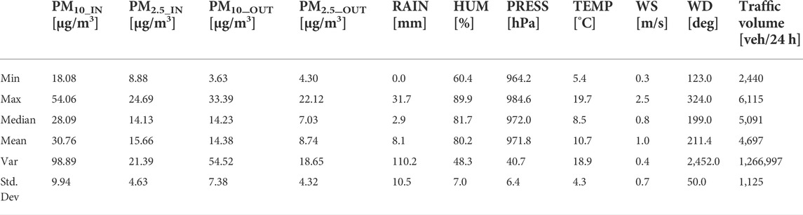
TABLE 1. Statistical characteristics of PM, meteorological conditions, and traffic volume (RAIN—precipitation, HUM—humidity, PRESS—pressure, TEMP—temperature, WS—wind speed, and WD—wind direction).
PM distribution in the tunnel tube represented the composition of PM10 by the fractions PM2.5_IN 51 % and PM2.5-10_IN 49 % near the portal part of PM2.5_OUT 59 % and PM2.5-10_OUT 41 %, respectively. The coarse fraction of PM2.5-10 reached up to 50 % of the total PM10 fraction. PM2.5-10 coarse particles can come mainly from abrasion of vehicle parts (brake wear, tire wear, clutch, and bodywork), road wear, and road dust re-suspension. The high proportion of coarse fractions indicates the presence of particles originating from abrasion (Fenger et al., 1998; OECD, 2020; Harrison et al., 2021). In the urban environment, the proportion of the coarse fraction PM2.5-10 can range from 12 %–54 % of the total fraction of PM10, whereas a larger proportion (≥50 %) is associated with intensive road traffic (Jandacka and Durcanska, 2019, 2021).
Road traffic is characterized by basic parameters such as traffic volume (the proportion of trucks), density, and speed of traffic flow (Cingel et al., 2019; Drliciak et al., 2020). In the tunnel tube where the PM measurements were performed, the traffic volume was recorded as 2,280 veh/24 h on average, and in the other tunnel tube, it was 2,428 veh/24 h on average. This represents a difference of 148 veh/24 h. As for the share of trucks in the traffic flow, in the tunnel tube where the PM measurements took place, this share was 42 %, and in the other tunnel tubes, it was 40 %. The traffic volume and traffic flow composition in the two tunnel tubes were not significantly different. The prevailing winds were from the south or southwest, from the direction of the bridge connected to the tunnel (Figure 1; Table 1).
A graphical evaluation of PM concentrations was performed using 24-h moving averages for the period before tunnel maintenance from 1/10/2020 to 7/10/2020 (Figure 2) and after tunnel maintenance from 13/10/2020 to 20/10/2020 (Figure 3). Hourly PM values obtained by continuous analyzers Fidas 200S and APM-2 were used for the evaluation. Table 1 shows the precipitation values as a total for 24 h (1 day). In the case of Figures 2, 3, the amount of precipitation is shown as a 24-h moving sum. Given a series of numbers and a fixed subset size, the first element of the moving average is obtained by taking the average of the initial fixed subset of the number series. Then, the subset was modified by “shifting forward”; that is, excluding the first number of the series and including the next value in the subset. Serial number 1 in Figure 2 is identical to the 24-h average value 01/10/2020 00:00–01/10/2020 23:00, respectively, in Figure 3 13/10/2020 00:00–13/10/2020 23:00. The decrease in traffic volume was reflected in the decrease in PM concentrations, especially in the tunnel tube over the weekend days: 3.10.2020–4.10.2020 (25–72) (Figure 2) and 17.10.2020–18.10.2020 (73–120) (Figure 3). The decrease in traffic volume on these days was 45 % compared to working days. The decrease in PM10 concentrations inside the tunnel on weekends averaged 5.3 % and PM2.5 at 13.1 %.
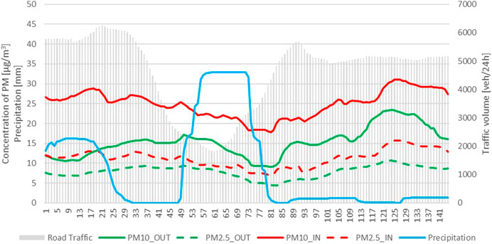
FIGURE 2. Trend of PM concentrations, traffic volume, and total precipitation during measurements in the Považský Chlmec tunnel in the period of 1/10/2020–7/10/2020.
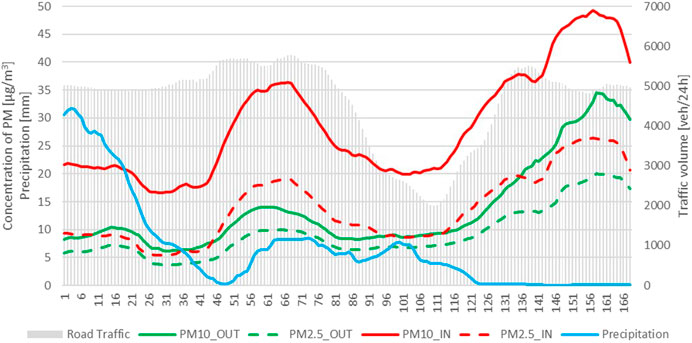
FIGURE 3. Trend of PM concentrations, traffic volume, and total precipitation during measurements in the Považský Chlmec tunnel in the period of 13/10/2020–20/10/2020.
PM measurements in the tunnel and outside near the tunnel portal were affected by heavy precipitation, which was reflected in the lower PM concentrations (Figures 2, 3). Precipitation affected PM concentrations by wet deposition, which also affected the distribution of particles inside and outside the tunnel (cleaner road surface, vehicles, and reduced re-suspension).
The average decreases in PM10 and PM2.5 concentrations during the days with precipitation compared to the days without precipitation were 45.4 % and 42.8 % outside the tunnel portal and 25.9 % and 28.9 % inside the tunnel, respectively. Standard tunnel maintenance and cleaning did not have a positive effect on the change in PM concentration. The average PM concentrations before maintenance were as follows, PM10_IN 28.2 μg/m3, PM2.5_IN 14.1 μg/m3, PM10_OUT 15.7 μg/m3, and PM2.5_OUT 7.1 μg/m3. The average PM concentrations after maintenance were as follows: PM10_IN 32.8 μg/m3, PM2.5_IN 16.9 μg/m3, PM10_OUT 13.3 μg/m3, and PM2.5_OUT 10.0 μg/m3.
The dependence of the PM measured in the tunnel tube and portal part of the tunnel was investigated using linear regression analysis. 24-h PM concentrations were used. The fine fraction PM2.5 showed a higher dependence of the particles produced in the tunnel tube on the particles measured in the portal part (coefficient of determination R2 = 0.57, correlation coefficient r = 0.75, and significance p = 0.005647) (Figure 4). This is because of the greater transport ability of the fine fraction, with PM entering the portal sections and outside air from the tunnel tube by natural or forced ventilation. For the coarse fraction PM2.5–10, the relationship between the particles measured in the tunnel tube and in the portal section was not as significant as for that of PM2.5 (R2 = 0.27, r = 0.52, p = 0.038899) (Figure 4). As the PM10 fraction contains fine PM2.5 and coarse PM2.5–10 components, it is affected by both. Therefore, the effect of PM10 produced inside the tunnel on PM10 concentrations outside near the tunnel portal was something between PM2.5 and PM2.5–10 and was significant (R2 = 0.43, r = 0.66, and p = 0.005647) (Figure 4).
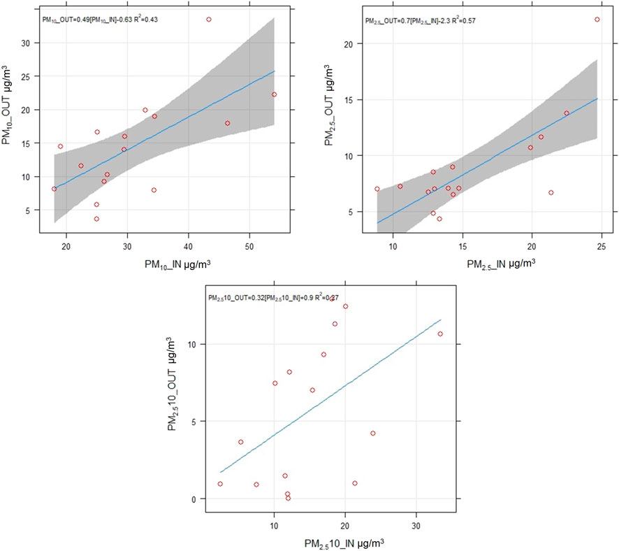
FIGURE 4. Results of the regression analysis performed for PM10, PM2.5, and PM2.5-10 concentrations during measurements in the Považský Chlmec tunnel (IN—inside the tunnel, OUT—outside near the tunnel portal).
3.2 Chemical analysis of particulate matter
Chemical analyses of PM revealed the presence of some chemical elements. 64 PM samples were analyzed, of which 32 PM10 samples and 32 PM2.5 samples. The following chemical elements were identified in PM: Al, Br, Ca, Cl, Cr, Cu, Fe, K, Mg, Mn, Na, P, Si, S, Ti, Zn, Ni, Mo, Pb, Rb, Sb, Se, Sr, V, and Zr. The total concentration of the elements on the filters averaged PM10_IN 365.8 mg/m2, PM2.5_IN 85.4 mg/m2, PM10_OUT 142.5 mg/m2, and PM2.5_OUT 48.2 mg/m2.
Below is a spectrum displayed by the ARL QUANT’X acquired from the PM samplings, filters T29, T30, and T31, with the elements of interest identified (Figure 5). Samples of PM10 T29, T30, and T31 were collected on 1/10/2020, 2/10/2020, and 3/10/2020, respectively.
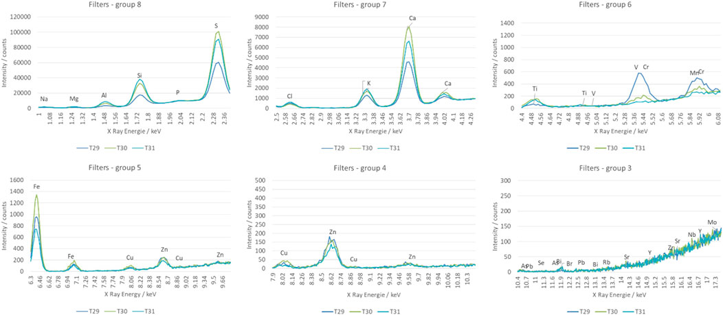
FIGURE 5. Spectrum of elements obtained by EDXRF in selected PM10 samples (T29, T30, and T31) during measurements in the Považský Chlmec tunnel.
The concentrations of chemical elements were higher inside the tunnel than outside, near the tunnel portal. For further evaluation and analysis, we focused on the chemical elements that met the criterion of the presence of at least 50 % of the samples (Al, Br, Ca, Cl, Cr, Cu, Fe, K, Mg, Mn, Na, P, Si, S, Ti, and Zn) (Figure 6). In general, the highest average concentration of ≥100 mg/g was recorded for the chemical elements Ca, Fe, Si, and S in the PM10 fraction inside the tunnel (Figure 6). Statistical evaluations of the minimum value, maximum value, mean, median, standard deviation, and variance are given in Supplementary Table S2. We recorded a decrease in the concentrations of chemical elements >50 % outdoors near the tunnel portal compared to concentrations inside the tunnel at Al, Ca, Cl, Cr, Cu, Fe, Mn, Na, Si, Ti, and Zn in PM10 and Ca, Cr, Cu, Fe, Na, P, and Ti in PM2.5, respectively (Figure 6).
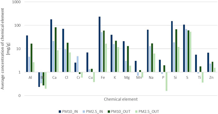
FIGURE 6. Average concentration of chemical elements in PM (milligrams of element per gram PM) during measurements in the Považský Chlmec tunnel.
The concentrations of chemical elements were also affected by precipitation that occurred during the measurements. A decrease in concentrations of chemical elements >50 % found outside near the tunnel portal during days with precipitation compared to days without precipitation was recorded for elements Al, Ca, Mg, and Si in PM10 and Ca, Mg, and Zn in PM2.5.
We also examined the representation of individual chemical elements in PM2.5 and PM2.5–10. PM2.5–10 represents the coarse fraction of PM10, and its source is mainly a mechanical process. The chemical elements Al, Ca, Cl, Cu, Fe, K, Mg, Mn, Na, P, Si, Ti, and Zn were present in the PM2.5–10 fraction to a greater extent (PM2.5–10/PM2.5 > 1). On the other hand, Br, Cr, S, K—outside, and Zn—outside were more represented in PM2.5 (ratio PM2.5-10/PM2.5 < 1) (Supplementary Table S2).
Correlation analysis was used to evaluate the presence and relationship of chemical elements in the PM fractions. The concentrations of the chemical elements in PM10, PM2.5, and PM2.5–10 were examined separately (Figure 7). The data obtained inside and outside the tunnel portal were combined for the correlation analysis. This created a data matrix measuring 17 × 32 (variables × observations). In this plot (Figure 7), the correlation coefficients are colored according to their values. Positive correlations are displayed in blue and negative correlations are shown in red. The color intensity and size of the circle were proportional to the correlation coefficients. On the right side of the correlogram, the legend shows the correlation coefficients and corresponding colors. The output of the correlation analysis was performed in R using the function chart. Correlation () is shown in Supplementary Figures S1–S3, which contain more information. The distribution of each variable is illustrated diagonally. Bivariate scatter plots are displayed with a fitted line at the bottom of the diagonal. At the top of the diagonal, the value of the correlation and significance level are shown as stars. Each significance level is associated with a symbol: p-values (0, 0.001, 0.01, 0.05, 0.1, and 1) ≤> symbols (“***,” “**,” “*,” “.“, and “”). −1 indicates a strong negative correlation, which means that every time x increases, y decreases. Zero indicates no association between the two variables (x and y). One indicates a strong positive correlation, suggesting that y increases with x.
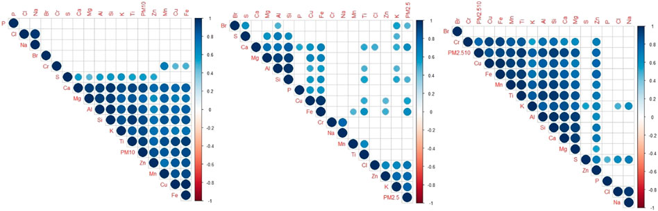
FIGURE 7. Results of correlation analysis of the concentration of chemical elements in PM obtained during measurements in the Považský Chlmec tunnel.
Correlation analysis revealed in PM10 two groups of chemical elements with significant mutual correlation (r > 0.7, p < 0.05): Group 1, Al, Ca, Cu, Fe, K, Mg, Mn, Si, Ti, and Zn; and Group 2, Na and Cl. In PM2.5, Al, Ca, Mg, Si, Cu, Fe, Na, and Cr were significantly correlated. In the PM2.5 fraction, the chemical elements were not as significantly bound as in the PM10 fraction. Thus, it was assumed that the coarse fraction PM2.5–10 was vital in the significant correlations between chemical elements. Therefore, this fraction was investigated separately. Significant correlations formed elements similar to the PM10 fraction (Figure 7). From the perspective of the interconnection of chemical elements, coarse fraction PM2.5–10 was significant for the total fraction PM10 in this case. Together with information about the representation of individual chemical elements in the fine or coarse fractions of PM, the correlation analysis provides a critical view of the internal structure of the PM chemical composition. Therefore, from the point of view of identifying and determining the source contribution to the production of PM, we can assume the origin of chemical elements and PM, especially in road traffic-related non-exhaust processes. The following section presents a detailed analysis of the source contributions to creating PM10 and PM2.5.
3.3 Source contribution to PM10 and PM2.5
A data matrix comprised of 17 variables and 32 observations were compiled for PCA and FA analyses. Measurements performed inside the tunnel (16 measurements) and outside the tunnel portal (16 measurements) were combined to achieve a suitable ratio of the number of observed variables (characters) and measurements (objects). The variables formed the concentrations of chemical elements found in PM10 and PM2.5, the concentrations of PM10 and PM2.5, and the observations formed on individual sampling days. After the first steps of the PM10 analysis, it was necessary to reduce the original matrix because of the poor indicators of the KMO and MSA criteria. The chemical elements Br, Cl, P, Cr, and Na, which reached the lowest values in the MSA criterion, were excluded from the matrix. Simultaneously, one remote measurement case was removed, which revealed a scatter plot of the component score from the PCA. The modified PM10 matrix comprised of 12 variables and 31 observations and was used as an input matrix for the calculation, with KMO = 0.85 and MSA (Table 2) reaching higher values. The data matrix for PM2.5 was adjusted based on low KMO and MSA criteria. The chemical elements Cl, P, Mn, Cr, and Na, which reached the lowest values in the MSA criterion, were excluded from the PM2.5 matrix. The modified PM2.5 matrix comprised of 12 variables and 32 observations was used as an input matrix for the calculation, with KMO = 0.77 and MSA (Table 2) reaching higher values.
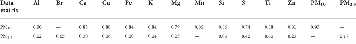
TABLE 2. Calculated MSA criteria values for variables in PM10 and PM2.5 data matrices.
As a first analysis, PCA was performed to obtain information about the internal structure of the data and to determine the number of significant PC.
Cattel’s scree plot is a bar graph of the eigenvalues λ1≥ λ2≥… ≥λm of the source data matrix X depending on the index i (Figure 8). Figure 8 shows the relative sizes of each eigenvalue. This is suitable for determining the number of “significant” PC. Non-significant PCs (factors) are represented in the horizontal bottom. Significant PCs are separated by a breakpoint, and the index value of this break indicates the number of significant components. In PM10, the first break can be indicated at index 2. Therefore, we used the first two PCs—PC1 and PC2. The criterion eigenvalue >1 can also be used, according to which we can choose the 2 PCs (Figure 8). The first two PCs (PC1 and PC2) explained 86.1 % of the total variance in PM10. In the following solution, the choice of the two PCs was justified, especially in terms of the interpretability of the factors. In the case of PM2.5, the first break is indicated by index 2 (Figure 9). In conjunction with the eigenvalue criterion of >1, the three main components, PC1, PC2, and PC3, were selected for further calculations. These three PCs (factors) characterized 82.4 % of the total variance for PM2.5 (Figure 9). A crucial decision in the FA is the number of factors to be extracted. The nFactors package in R was used, which offers a suite of functions to aid in this decision. Nonetheless, any factor solution must be interpretable for it to be valid.
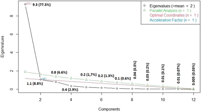
FIGURE 8. Scree plot for PM10 data matrix obtained by PCA analysis.
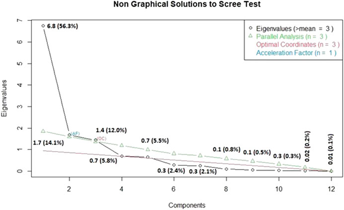
FIGURE 9. Scree plot for PM2.5 data matrix obtained by PCA analysis.
The plot of the component weight graph shows the component weights for the first two PCs (Figures 10A, C). Each point in the graph corresponds to one character, and the distances between characters are compared in the graph. A short distance between characters indicates a strong correlation. Most of the characters were placed in the graph point in the same direction from the beginning, indicating their positive correlation. The graph also shows that the percentage of the total variance of the data characterizes the first two PCs (Dim 1 and Dim 2) (Figures 10A,C). The double graph (biplot) combines the plot component weights, and the scatter plot of the component score (Figures 10B, D). The angle between the vectors of the two characters is directly proportional to the size of their correlation; the smaller the angle, the greater the correlation. For example, in the case of PM10, we can observe this for the variables such as Fe, Mn, and Cu (Figure 10B), or in the case of PM2.5, for the variables Mg and Si (Figure 10D). Each vector of the variable has a length that is proportional to the contribution of the original character to the main component, that is, proportional to the component weight. If there is an object near a certain character in the double graph, it means that this object “contains” a large proportion of this character and is interacting with it (e.g., characters Zn, Mg, Al, Si, Ca, and objects 14, 15 in PM10) (Figure 10B).
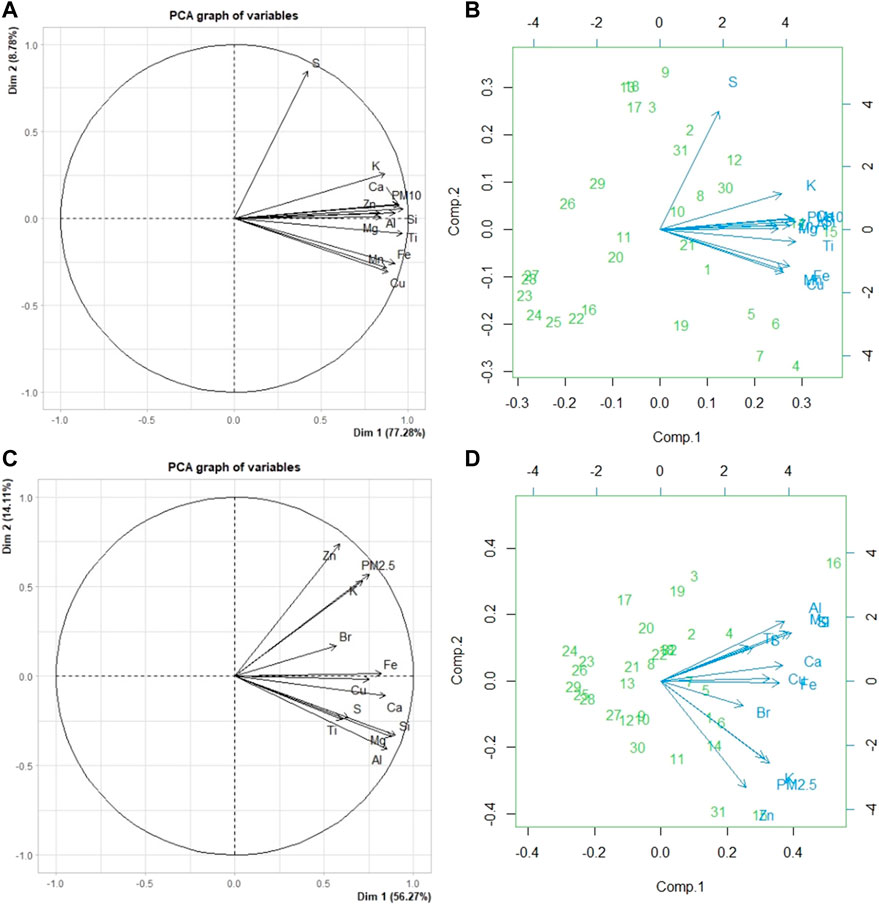
FIGURE 10. Plot component weights: PM10 (A); PM2.5 (C). Biplot: PM10 (B); PM2.5 (D) obtained by PCA analysis.
The previous PCA analysis was necessary for a basic understanding of the variance in the original features and to identify the appropriate number of latent variables. Thus, for the subsequent FA, two factors were selected for PM10 and three for PM2.5, and varimax rotation was used. The main goal of the rotation is to derive easily explainable and namable common factors from data. In this case, the rotating factors are chosen such that some loads reach high values, whereas others reach extremely low values. A simple structure was achieved by turning. A factor load criterion ≥0.7 was chosen to indicate the assignment of a character to a particular factor (Figures 11, 12). Based on assigning individual characters (chemical elements) to a given factor, its interpretation and naming as PM10 or PM2.5 sources are possible. This interpretation is also based on the knowledge of the possible sources of individual chemical elements, which are available from various others and on studies devoted to the chemical composition of PM. (Yli-Tuomi et al., 2005; Thorpe and Harrison, 2008; Cui et al., 2016; Harrison et al., 2021; Jandacka and Durcanska, 2021). Based on these assumptions, PM10 sources in the tunnel environment were interpreted as follows: Factor 1—Brake and tire wear (Cu, Fe, Mn, Ti, Zn, PM10); Factor 2—Road wear, re-suspension, and exhaust emissions (Al, Ca, K, Mg, and Si) (Figure 11), and PM2.5, sources as follows: Factor 1—Road wear and re-suspension (Al, Mg, Si, and S), Factor 2—Break wear (Cu, Fe), Factor 3—Exhaust emissions and tire wear (K, Zn, and PM2.5) (Figure 12). The interpretation of these PM10 and PM2.5 sources is based on the facts concerning the sampling point itself—the tunnel environment. The sources of PM10 and PM2.5 in the tunnel are road traffic. Therefore, it is an ideal environment for diversifying PM10 and PM2.5, sub-sources from road traffic, and determining their contribution to PM10 and PM2.5.
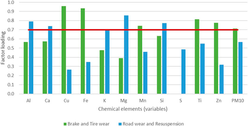
FIGURE 11. Factor loadings of variables (chemical elements and PM) to factors (PM sources) for data matrix PM10 obtained by FA.
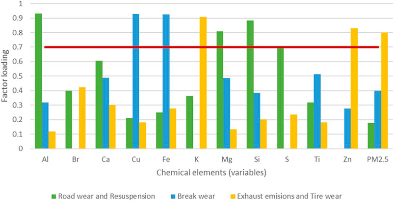
FIGURE 12. Factor loadings of variables (chemical elements and PM) to factors (PM sources) for data matrix PM2.5 obtained by FA.
The APCS with the MRA method was used to estimate the contribution of the identified sources to the production of PM10 and PM2.5. By using an MRA, where PM is a dependent variable, and APCS is an independent variable, contributions from individually identified sources can be obtained. These were calculated from the regression coefficients obtained by multiplying them by the average APCS value for each common factor as an absolute contribution, which was converted from the total PM concentration to the percentage source contribution.
All variables (factors) are significant in the model (** or ***) and contribute significantly to PM10 and PM2.5 concentrations (Table 3). The coefficient of determination describes the proportion of total variance, which can be explained by a linear relationship. In the case of PM10, it has the value R2 = 0.83 and PM2.5 R2 = 0.97, which means that the linear relationship clarifies a sufficiently large part of the total variance. The level of significance is negligible; therefore, the use of the given model is sufficiently significant for PM10 p = 1.39e−16 and PM2.5 P = <2.2e−16.
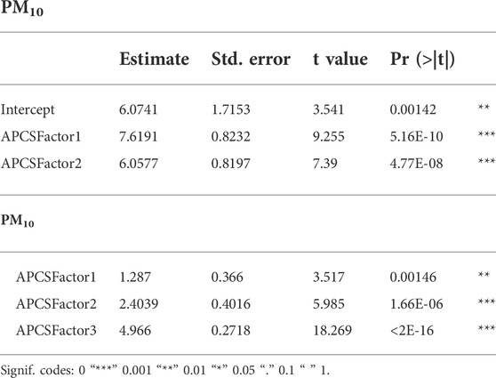
TABLE 3. Results of the MRA model for evaluating the source contribution.
The average absolute factor contributions and the average percentage factor contributions relate to the average concentration of PM10 21.55 μg/m3 and PM2.5 12.20 μg/m3 from all analyzed data.
According to the results of the APCS analysis, the sources of road wear and re-suspension contributed the most to the average PM10 concentration at a value of 10.34 μg/m3, representing a 48 % share of the average PM10 concentration. Source: Brake and tire wear contributed to the average PM10 concentration with an absolute value of 5.14 μg/m3, representing a 24 % share of the average PM10 concentration. The undifferentiated part contributed to an average PM10 concentration of 6.1 μg/m3, which is 28 %.
According to the results of the APCS analysis, the source contributed the most to the average PM2.5 concentration, exhaust emissions, and tire wear, 9.07 μg/m3, which represented a 75.9 % share of the average PM2.5 concentration. Source: Road wear and re-suspension contribute to the average PM2.5 concentration with an absolute value of 1.45 μg/m3, representing a 12.1 % share of the average PM2.5. Source: Break wear contributes to an average PM2.5 concentration of 1.43 μg/m3, representing 12.0 % of the average PM2.5.
4 Conclusion
The present research dealt with the measurement and analysis of PM10 and PM2.5 concentrations and their chemical compositions in a tunnel environment. The measurement site was the Považský Chlmec tunnel located in Žilina, Slovakia. The measurements were performed inside the tunnel tube and outside near the tunnel portal, which differs from other studies (Cui et al., 2016; Hao et al., 2019). The average concentration of PM10 in the tunnel was 53 % higher and that of PM2.5 44 % higher than that outside near the tunnel portal. The concentrations were significantly affected by precipitation during measurement. The impact of the primary road traffic source was manifested mainly during working days by an increase in PM concentrations which increased during the non-precipitation period. The regression analysis of PM concentrations inside the tunnel and outside near the tunnel portal showed the interconnection of these PMs; that is, a large part of the PM in the portal came directly from the tunnel (PM10—R2 = 0.43, PM2.5—R2 = 0.57). PM2.5-10 accounted for up to 50 % of the total PM10 fraction, which is a higher value than that of urban aerosols (Horvath et al., 1996; Chan and Kwok, 2001; Samara and Voutsa, 2005; Jandacka and Durcanska, 2021). Standard tunnel maintenance and cleaning did not have a positive effect on the change in PM concentration. This could be caused by significant precipitation during the measurement.
Chemical analysis of PM10 and PM2.5 using EDXRF revealed the presence of the following chemical elements in PM: Al, Br, Ca, Cl, Cr, Cu, Fe, K, Mg, Mn, Na, P, Si, S, Ti, and Zn. The total concentration of elements on the filters was in average for PM10_IN 365.8 mg/m2, PM2.5_IN 85.4 mg/m2, PM10_OUT 142.5 mg/m2, and PM2.5_OUT 48.2 mg/m2. These chemical elements were represented by weight in PM10_IN (31.4 %), PM2.5_IN (14.4 %), PM10_OUT (27.7 %), and PM2.5_OUT (15.4 %). Similar results of PM composition in tunnels have been obtained in some studies (Gillies et al., 2001; Handler et al., 2008; He et al., 2008; Brito et al., 2013; Cui et al., 2016; Hao et al., 2019). The concentrations of chemical elements reached higher values inside the tunnel than outside, near the tunnel portal.
The chemical composition of the PM was used to identify and estimate the contribution of the PM sources. FA, PCA, and APCS methods were used for this purpose. The results were processed for the PM10 and PM2.5 fractions (measurements inside the tunnel together with measurements outside near the tunnel portal). Based on the input data and the performed analyses, two sources for PM10 were identified with a calculated contribution: Factor 1—Brake and tire wear (24 %); Factor 2—Road wear, re-suspension, and exhaust emissions (48 %), and three sources for PM2.5, with calculated contributions: Factor 1–Road wear and re-suspension (12 %), Factor 2–break wear (12 %), Factor 3–Exhaust emissions and tire wear (76 %). The PM2.5-10 accounted for 50 % of the total PM10 fraction. The chemical elements Al, Ca, Cl, Cu, Fe, K, Mg, Mn, Na, P, Si, Ti, and Zn were more represented in PM2.5–10, which was also reflected in the evaluation of the contribution of resources in the PM10 fraction. These elements in PM2.5–10 originated from the mechanical wear of road traffic. On the other hand, the PM2.5 analysis showed that elements K and Zn can also come from exhaust processes in vehicles, as a high proportion of freight traffic of 40 % was recorded. A high proportion of sulfur in PM was found, which may be due to exhaust PM emissions (Agarwal, 2007; Liati et al., 2012; Pant and Harrison, 2013; Reşitoʇlu et al., 2015; Filonchyk et al., 2018; Chernyshev et al., 2019) as well as road surface wear (Yli-Tuomi et al., 2005; Thorpe and Harrison, 2008; Gustafsson, 2018; OECD, 2020; Jandacka et al., 2021). FA revealed a higher factor load of sulfur to the factor “road wear and re-suspension.” However, a factor load was also identified as the factor “exhaust emissions and tire wear” in the analysis of PM2.5. It is, therefore, essential to consider that the PM fraction of the FA and the analysis of the source contribution were carried out.
To the best of our knowledge, this is the first study dedicated to the quantification of PM properties and determination of source contribution using the methods presented in this particular tunnel in Slovakia. In the future, we plan to continue PM research in the tunnel environment and extend the measurements to the number and mass distribution of the “tunnel aerosol.” We will also focus on organic compounds in PM (benzo(a)pyrene, EC, and OC). These efforts could lead to a better understanding of the formation, composition, and development of traffic-related PM.
Data availability statement
The raw data supporting the conclusion of this article will be made available by the authors, without undue reservation.
Author contributions
DJ and DD contributed to conception and design of the study. DJ and DD made measurements. RC realized the chemical analysis. DJ evaluated measured the data. DJ performed the statistical analysis. DJ wrote the first draft of the manuscript. DJ, DD, and RC wrote sections of the manuscript. All authors contributed to manuscript revision, read, and approved the submitted version.
Funding
This study was supported by a VEGA 1/0337/22 grant entitled “Analysis of the influence of the pavement surface texture on skid friction, road safety, and the potential of road dust re-suspension.”
Conflict of interest
The authors declare that the research was conducted in the absence of any commercial or financial relationships that could be construed as a potential conflict of interest.
Publisher’s note
All claims expressed in this article are solely those of the authors and do not necessarily represent those of their affiliated organizations, or those of the publisher, the editors, and the reviewers. Any product that may be evaluated in this article, or claim that may be made by its manufacturer, is not guaranteed or endorsed by the publisher.
Supplementary material
The Supplementary Material for this article can be found online at: https://www.frontiersin.org/articles/10.3389/fenvs.2022.952577/full#supplementary-material
References
Agarwal, A. K. (2007). Biofuels (alcohols and biodiesel) applications as fuels for internal combustion engines. Prog. Energy Combust. Sci. 33, 233–271. doi:10.1016/J.PECS.2006.08.003
Allen, A., Nemitz, E., Shi, J., Harrison, R., and Greenwood, J. (2001). Size distributions of trace metals in atmospheric aerosols in the United Kingdom. Atmos. Environ. X. 35, 4581–4591. doi:10.1016/S1352-2310(01)00190-X
Almeida, S. M., Pio, C. A., Freitas, M. C., Reis, M. A., and Trancoso, M. A. (2006). Source apportionment of atmospheric urban aerosol based on weekdays/weekend variability: Evaluation of road re-suspended dust contribution. Atmos. Environ. X. 40, 2058–2067. doi:10.1016/j.atmosenv.2005.11.046
Alves, C. A., Evtyugina, M., Vicente, A. M. P., Vicente, E. D., Nunes, T. V., Silva, P. M. A., et al. (2018). Chemical profiling of PM10 from urban road dust. Sci. Total Environ. 634, 41–51. doi:10.1016/j.scitotenv.2018.03.338
Beelen, R., Hoek, G., van den Brandt, P. A., Goldbohm, R. A., Fischer, P., Schouten, L. J., et al. (2008). Long-term effects of traffic-related air pollution on mortality in a Dutch cohort (NLCS-AIR study). Environ. Health Perspect. 116, 196–202. doi:10.1289/ehp.10767
Bilos, C., Colombo, J. C., Skorupka, C. N., and Rodriguez Presa, M. J. (2001). Sources, distribution and variability of airborne trace metals in La Plata City area, Argentina. Environ. Pollut. 111, 149–158. doi:10.1016/s0269-7491(99)00328-0
Briliak, D., and Remišová, E. (2022). Stiffness modulus of aged asphalt mixtures. Solid State Phenom. 329, 93–100. doi:10.4028/P-PC709Y
Brito, J., Rizzo, L. V., Herckes, P., Vasconcellos, P. C., Caumo, S. E. S., Fornaro, A., et al. (2013). Physical–chemical characterisation of the particulate matter inside two road tunnels in the São Paulo Metropolitan Area. Atmos. Chem. Phys. 13, 12199–12213. doi:10.5194/acp-13-12199-2013
Chan, L. Y., and Kwok, W. S. (2001). Roadside suspended particulates at heavily trafficked urban sites of Hong Kong – Seasonal variation and dependence on meteorological conditions. Atmos. Environ. X. 35, 3177–3182. doi:10.1016/s1352-2310(00)00504-5
Celo, V., Yassine, M. M., and Dabek-Zlotorzynska, E. (2021). Insights into elemental composition and sources of fine and coarse particulate matter in dense traffic areas in toronto and vancouver, Canada. Toxics 9, 264. doi:10.3390/toxics9100264
Chellam, S., Kulkarni, P., and Fraser, M. P. (2011). Emissions of organic compounds and trace metals in fine particulate matter from motor vehicles: A tunnel study in houston, Texas. J. Air & Waste Manag. Assoc. 55, 60–72. doi:10.1080/10473289.2005.10464597
Chernyshev, V. V., Zakharenko, A. M., Ugay, S. M., Hien, T. T., Hai, L. H., Olesik, S. M., et al. (2019). Morphological and chemical composition of particulate matter in buses exhaust. Toxicol. Rep. 6, 120–125. doi:10.1016/J.TOXREP.2018.12.002
Cingel, M., Čelko, J., and Drličiak, M. (2019). Analysis in modal split. Transp. Res. Procedia 40, 178–185. doi:10.1016/J.TRPRO.2019.07.028
Cui, M., Chen, Y., Tian, C., Zhang, F., Yan, C., and Zheng, M. (2016). Chemical composition of PM2.5 from two tunnels with different vehicular fleet characteristics. Sci. Total Environ. 550, 123–132. doi:10.1016/J.SCITOTENV.2016.01.077
de la Paz, D., Borge, R., Vedrenne, M., Lumbreras, J., Amato, F., Karanasiou, A., et al. (2015). Implementation of road dust resuspension in air quality simulations of particulate matter in Madrid (Spain). Front. Environ. Sci. 3 72. doi:10.3389/fenvs.2015.00072
Drliciak, M., Celko, J., Cingel, M., and Jandacka, D. (2020). Traffic volumes as a modal split parameter. Sustainability 12, 10252. doi:10.3390/SU122410252
Dziuban, C. D., and Shirkey, E. C. (1974). When is a correlation matrix appropriate for factor analysis? Some decision rules. Psychol. Bull. 81, 358–361. doi:10.1037/H0036316
Fenger, J., Jes), , Hertel, O., and Palmgren, F. (1998). Urban air pollution - European aspects. Berlin, Germany: Springer Science & Business Media, 482.
Filonchyk, M., Yan, H., and Li, X. (2018). Temporal and spatial variation of particulate matter and its correlation with other criteria of air pollutants in Lanzhou, China, in spring-summer periods. Atmos. Pollut. Res. 9, 1100–1110. doi:10.1016/j.apr.2018.04.011
Fullova, D., Durcanska, D., Jandacka, D., and Estokova, A. (2016). Mass distribution of particulate matter produced during abrasion af asphalt mixtures in laboratory. Communications 18, 37–43. doi:10.26552/com.c.2016.4.37-43
Gillies, J. A., Gertler, A. W., Sagebiel, J. C., and Dippel, W. A. (2001). On-road particulate matter (PM2.5 and PM10) emissions in the sepulveda tunnel, los angeles, California. Environ. Sci. Technol. 35, 1054–1063. doi:10.1021/ES991320P
Guo, H., Wang, T., and Louie, P. K. K. (2004). Source apportionment of ambient non-methane hydrocarbons in Hong Kong. Environ. Pollut. 129, 489–498. doi:10.1016/j.envpol.2003.11.006
Gustafsson, M. (2018). “Review of road wear emissions,” in Non-exhaust emissions (Amsterdam, Netherlands: Elsevier), 161–181. doi:10.1016/B978-0-12-811770-5.00008-X
Handler, M., Puls, C., Zbiral, J., Marr, I., Puxbaum, H., and Limbeck, A. (2008). Size and composition of particulate emissions from motor vehicles in the Kaisermühlen-Tunnel, Vienna. Atmos. Environ. X. 42, 2173–2186. doi:10.1016/J.ATMOSENV.2007.11.054
Hao, Y., Deng, S., Yang, Y., Song, W., Tong, H., and Qiu, Z. (2019). Chemical composition of particulate matter from traffic emissions in a road tunnel in xi’an, China. Aerosol Air Qual. Res. 19, 234–246. doi:10.4209/AAQR.2018.04.0131
Harrison, R. M., Allan, J., Carruthers, D., Heal, M. R., Lewis, A. C., Marner, B., et al. (2021). Non-exhaust vehicle emissions of particulate matter and VOC from road traffic: A review. Atmos. Environ. X. 262, 118592. doi:10.1016/J.ATMOSENV.2021.118592
He, L. Y., Hu, M., Zhang, Y. H., Huang, X. F., and Yao, T. T. (2008). Fine particle emissions from on-road vehicles in the Zhujiang Tunnel, China. Environ. Sci. Technol. 42, 4461–4466. doi:10.1021/ES7022658/SUPPL_FILE/ES7022658-FILE003
Hildemann, L. M., Markowski, G. R., and Cass, G. R. (1991). Chemical composition of emissions from urban sources of fine organic aerosol. Environ. Sci. Technol. 25, 744–759. doi:10.1021/ES00016A021/SUPPL_FILE/ES00016A021_SI_001
Horvath, H., Kasahara, M., and Pesava, P. (1996). The size distribution and composition of the atmospheric aerosol at a rural and nearby urban location. J. Aerosol Sci. 27, 417–435. doi:10.1016/0021-8502(95)00546-3
Jain, S., Sharma, S. K., Mandal, T. K., and Saxena, M. (2018). Source apportionment of PM10 in Delhi, India using PCA/APCS, UNMIX and PMF. Particuology 37, 107–118. doi:10.1016/J.PARTIC.2017.05.009
Jandacka, D., Durcanska, D., and Bujdos, M. (2017). The contribution of road traffic to particulate matter and metals in air pollution in the vicinity of an urban road. Transp. Res. Part D Transp. Environ. 50, 397–408. doi:10.1016/j.trd.2016.11.024
Jandacka, D., and Durcanska, D. (2019). Differentiation of particulate matter sources based on the chemical composition of PM10 in functional urban areas. Atmos. (Basel) 10, 583. doi:10.3390/atmos10100583
Jandacka, D., and Durcanska, D. (2021). Seasonal variation, chemical composition, and PMF-derived sources identification of traffic-related PM1, PM2.5, and pm2.5–10 in the air quality management region of Žilina, Slovakia. Int. J. Environ. Res. Public Health 18, 10191. doi:10.3390/IJERPH181910191
Jandacka, D., Kovalova, D., Durcanska, D., and Decky, M. (2021). Chemical composition, morphology, and distribution of particulate matter produced by road pavement abrasion using different types of aggregates and asphalt binder. Cogent Eng. 8, 1884325. doi:10.1080/23311916.2021.1884325
Jandačka, D. (2015). Sources of PM 10 air pollution in rural area in the vicinity of a highway in Žilina selfgoverning region, Slovakia. Civ. Environ. Eng. 11, 58–68. doi:10.1515/CEE-2015-0008
Kaiser, H. F., and Rice, J. (2016). Little jiffy, mark iv. Educ. Psychol. Meas. 34, 111–117. doi:10.1177/001316447403400115
Kennedy, P., and Gadd, J. (2000). Preliminary examination of trace elements in tyres, brake pads and road bitumen in New Zealand.
Kováč, M., Brna, M., and Decký, M. (2021). Pavement friction prediction using 3D texture parameters. Coatings 11, 1180. doi:10.3390/COATINGS11101180
Legret, M., and Pagotto, C. (1999). Evaluation of pollutant loadings in the runoff waters from a major rural highway. Sci. Total Environ. 235, 143–150. doi:10.1016/S0048-9697(99)00207-7
Leitner, B., Decký, M., and Kováč, M. (2019). Road pavement longitudinal evenness quantification as stationary stochastic process. Transport 34, 193–203. doi:10.3846/transport.2019.8577
Liati, A., Dimopoulos Eggenschwiler, P., Müller Gubler, E., Schreiber, D., and Aguirre, M. (2012). Investigation of diesel ash particulate matter: A scanning electron microscope and transmission electron microscope study. Atmos. Environ. X. 49, 391–402. doi:10.1016/J.ATMOSENV.2011.10.035
Lu, X., Wang, L., Li, L. Y., Lei, K., Huang, L., and Kang, D. (2010). Multivariate statistical analysis of heavy metals in street dust of Baoji, NW China. J. Hazard. Mat. 173, 744–749. doi:10.1016/J.JHAZMAT.2009.09.001
Manta, D. S., Angelone, M., Bellanca, A., Neri, R., and Sprovieri, M. (2002). Heavy metals in urban soils: A case study from the city of palermo (sicily), Italy. Sci. Total Environ. 300, 229–243. doi:10.1016/S0048-9697(02)00273-5
Morabito, E., Gregoris, E., Belosi, F., Contini, D., Cesari, D., and Gambaro, A. (2020). Multi-year concentrations, Health risk, and source identification, of air toxics in the venice lagoon. Front. Environ. Sci. 8. doi:10.3389/fenvs.2020.00107
OECD (2020). Non-exhaust particulate emissions from road transport: An Ignored Environmental Policy Challenge. Paris: OECD Publishing 149. doi:10.1787/4a4dc6ca-en
Pant, P., and Harrison, R. M. (2013). Estimation of the contribution of road traffic emissions to particulate matter concentrations from field measurements: A review. Atmos. Environ. X. 77, 78–97. doi:10.1016/j.atmosenv.2013.04.028
Pope, C. A. (2002). Lung cancer, cardiopulmonary mortality, and long-term exposure to fine particulate air pollution. JAMA 287, 1132. doi:10.1001/jama.287.9.1132
Reşitoʇlu, I. A., Altinişik, K., and Keskin, A. (2015). The pollutant emissions from diesel-engine vehicles and exhaust aftertreatment systems. Clean. Technol. Environ. Policy 17, 15–27. doi:10.1007/s10098-014-0793-9
Rexeis, M., and Hausberger, S. (2009). Trend of vehicle emission levels until 2020 – prognosis based on current vehicle measurements and future emission legislation. Atmos. Environ. X. 43, 4689–4698. doi:10.1016/J.ATMOSENV.2008.09.034
Samara, C., and Voutsa, D. (2005). Size distribution of airborne particulate matter and associated heavy metals in the roadside environment. Chemosphere 59, 1197–1206. doi:10.1016/J.CHEMOSPHERE.2004.11.061
Samoli, E., Peng, R., Ramsay, T., Pipikou, M., Touloumi, G., Dominici, F., et al. (2008). Acute effects of ambient particulate matter on mortality in europe and north America: Results from the APHENA study. Environ. Health Perspect. 116, 1480–1486. doi:10.1289/ehp.11345
Širilla, M., and Schmidt, P. (2017). D3 Žilina (Strážov) - Žilina (brodno), Považský Chlmec tunnel. Inžinierske stavby (Engineering Constr. 6/2017.
Soleimani, M., Amini, N., Sadeghian, B., Wang, D., and Fang, L. (2018). Heavy metals and their source identification in particulate matter (PM2.5) in Isfahan City, Iran. J. Environ. Sci. 72, 166–175. doi:10.1016/j.jes.2018.01.002
Song, Y., Xie, S., Zhang, Y., Zeng, L., Salmon, L. G., and Zheng, M. (2006). Source apportionment of PM2.5 in Beijing using principal component analysis/absolute principal component scores and UNMIX. Sci. Total Environ. 372, 278–286. doi:10.1016/J.SCITOTENV.2006.08.041
Tahri, M., Benyaïch, F., Bounakhla, M., Bilal, E., Gruffat, J. J., Moutte, J., et al. (2005). Multivariate analysis of heavy metal contents in soils, sediments and water in the region of Meknes (Central Morocco). Environ. Monit. Assess. 102, 405–417. doi:10.1007/S10661-005-6572-7
Thorpe, A., and Harrison, R. M. (2008). Sources and properties of non-exhaust particulate matter from road traffic: A review. Sci. Total Environ. 400, 270–282. doi:10.1016/J.SCITOTENV.2008.06.007
Timmers, V. R. J. H., and Achten, P. A. J. (2016). Non-exhaust PM emissions from electric vehicles. Atmos. Environ. X. 134, 10–17. doi:10.1016/J.ATMOSENV.2016.03.017
Tokalioǧlu, Ş., and Kartal, Ş. (2006). Multivariate analysis of the data and speciation of heavy metals in street dust samples from the Organized Industrial District in Kayseri (Turkey). Atmos. Environ. X. 40, 2797–2805. doi:10.1016/j.atmosenv.2006.01.019
US-EPA (2011). AP-42, 5th edn., vol. 1, chapter 13 miscellaneous sources., section 13.2.1 paved roads. Available at: https://www.epa.gov/sites/default/files/2020-10/documents/13.2.1_paved_roads.pdf (Accessed May 23, 2022).
WHO (2007). “Health relevance of particulate matter from various sources,” in Report on a WHO workshop, Bonn, Germany, March 26–27, 2007 (Copenhagen: WHO Regional Office for Europe) Available at: https://apps.who.int/iris/bitstream/handle/10665/107846/E90672.pdf.
World Health Organization (2013). HealtH effects of particulate matter. Available at: http://www.euro.who.int/pubrequest (Accessed July 9, 2021).
Yang, H. H., Dhital, N. B., Wang, L. C., Hsieh, Y. S., Lee, K. T., Hsu, Y. T., et al. (2019). Chemical characterization of fine particulate matter in gasoline and diesel vehicle exhaust. Aerosol Air Qual. Res. 19, 1439–1449. doi:10.4209/AAQR.2019.04.0191
Yang, Z., Lu, W., Long, Y., Bao, X., and Yang, Q. (2011). Assessment of heavy metals contamination in urban topsoil from Changchun City, China. J. Geochem. Explor. 108, 27–38. doi:10.1016/J.GEXPLO.2010.09.006
Keywords: particulate matter, non-exhaust emissions, chemical element, tunnel environment, road traffic, factor analysis
Citation: Jandacka D, Durcanska D and Cibula R (2022) Concentration and inorganic elemental analysis of particulate matter in a road tunnel environment (Žilina, Slovakia): Contribution of non-exhaust sources. Front. Environ. Sci. 10:952577. doi: 10.3389/fenvs.2022.952577
Received: 25 May 2022; Accepted: 07 September 2022;
Published: 30 September 2022.
Edited by:
Cristian Focsa, Université de Lille, FranceReviewed by:
Adalgiza Fornaro, University of São Paulo, BrazilAmin Ismael Nawahda, Palestine Technical University Kadoorie, Palestine
Copyright © 2022 Jandacka, Durcanska and Cibula. This is an open-access article distributed under the terms of the Creative Commons Attribution License (CC BY). The use, distribution or reproduction in other forums is permitted, provided the original author(s) and the copyright owner(s) are credited and that the original publication in this journal is cited, in accordance with accepted academic practice. No use, distribution or reproduction is permitted which does not comply with these terms.
*Correspondence: Dusan Jandacka, ZHVzYW4uamFuZGFja2FAdW5pemEuc2s=