 Yan Zhou
 Liangjie Zhao
 Jianwen Cao2
95% of researchers rate our articles as excellent or good
Learn more about the work of our research integrity team to safeguard the quality of each article we publish.
Find out more
ORIGINAL RESEARCH article
Front. Environ. Sci. , 22 July 2022
Sec. Freshwater Science
Volume 10 - 2022 | https://doi.org/10.3389/fenvs.2022.950098
This article is part of the Research Topic Interactions between Groundwater and Human Communities: Perspectives on the Resources, Environments, Threats and Sustainable Development View all 18 articles
Hydrological simulation of the karst area is significant for assessing water resources accurately and exploring the relationship in the hydrologic cycle. However, the existence of sinkholes causes the spatial heterogeneity of aquifers and changes the distribution of surface water as well as groundwater, which makes the traditional hydrogeological model difficult to quantitatively characterize the hydrological processes of the sinkhole. Hence, improving the hydrological model for the karst area is a necessary direction at present. The soil and water assessment tool (SWAT) is one of the most widely used semi-distributed hydrological models right now in the world. In this study, we focused on the upper course of the South Panjiang River and used the pond module of the SWAT model to simulate karst sinkholes, modifying the source code to realize the rapid response to the recharge in karst sinkholes. After the improvement, the surface runoff, especially the peak value of the Xiqiao Hydrological Station at the outlet, has been reduced, while the baseflow of modified subbasins has been increased and the water yield is under a state of water balance. In addition, the model evaluation factor R2 was strengthened from 0.76 to 0.83 and NSE was strengthened from 0.66 to 0.79 of the Xiqiao Hydrological Station during the validation period. The improved model was used to analyze the spatial distribution of hydrological components. Also, it was found there are spatial relations between runoff modulus–slope and baseflow–surface runoff–land use types. The analysis demonstrated that the improved SWAT model could effectively change the hydrological components and simulate the rapid replenishment of karst sinkholes.
Karst is a special landscape shape, which can be classified into carbonate karst, evaporate karst, and sandstone karst according to the constituting material (Veress 2020). It develops mainly with groundwater solution of the carbonate rocks when groundwater flows, which exports the products of dissolution, creating underground voids, and the processes can develop a hydraulic continuum from the surface to spring (Bakalowicz 2005). Karst is widely distributed in Southwest China, and a lot of research on karst has been carried out in these areas, including determining the output characteristics of fissure flows (Li et al., 2020), estimating groundwater storage and detecting anomalies in karstic regions (Huang et al., 2019), and investigating the influence of climatic variability on solute dynamics (Liu et al., 2020).
The karst aquifer and epikarst are indispensable parts of the karst area. The karst aquifer constitutes an important source of water supply. Ford and Williams, (2007) estimated that 7–10% of the planet is karst and roughly 20–25% of the global population depends largely or entirely on groundwater obtained from them. Typical epikarst phenomena such as spring, cave, sinkhole, and depression are present under the erosion of water flow. Among them, sinkholes develop where the rock in the karstic area undergoes chemical weathering or dissolution through groundwater movement and infiltration of surface water or precipitation (Cahalan and Milewski 2015).
However, modeling karst systems is still a complex task and has been the subject of continuing research globally. A difficulty is that the geometry of fractures, the position of conduits, and the interactions between different types of flows are unknown in many cases (Salerno and Tartari 2009). As an important method, the hydrological model emerges as time requires. Three types of mathematical hydrological models can be applied for the karst flow simulation: theoretical or physical models, conceptual models, and empirical or black-box models (Deni-Juki and Juki 2003). The simplest way to model karst hydrology is the application of “black-box” models. They transfer input to output without the explicit representation of any physical processes and ignore the complexity of the aquifer geometry (Halihan and Wicks 1998). The KAGIS model, artificial neural network model, and regression model were used to simulate and predict the hydrodynamic behavior of karst aquifers (Felton and Currens 1994; Lallahem et al., 2005; Hu et al., 2008; Valdes-Abellan et al., 2018; Nhu et al., 2020). However, the results lose their reliability outside the range of conditions they were calibrated for (Hartmann et al., 2014). Moreover, it requires long time series of input data, which is difficult for the data-starved area (Meng and Wang 2010).
The conceptual model is based on a set of equations transferring input to output, conceptually representing physical processes, and it is widely used in karst modeling due to easy implementation (Hartmann et al., 2012). The Hydrological Model for Karst Environment (HYMKE) (Rimmer and Salingar 2006; Samuels et al., 2010), Génie Rural à 4 paramètres Journalier (GR4J) (Sezen et al., 2019), and Karst Simulation Simplified (K sim2) model (Makropoulos et al., 2008) are successfully applied in the karst area. However, this kind of model often discards details in the system dynamics to simplify the model, and it is difficult to be applied to large-scale basins (Meng and Wang 2010). For the quantitative spatial simulation in large-scale watersheds, conceptual models are less advantageous than physical models (Martínez-Santos and Andreu 2010).
The physics-based numerical model generally ignores the complexity of karst aquifer geometry and interprets the response with mathematical techniques and empirical assumptions. These approaches can also simplify the conduit geometry and interpret the response that the system will generate (Halihan and Wicks 1998). Karst areas usually lack data and have a complex structure, and the distributed and semi-distributed models have advantages. This kind of model allows grid refinement, and its structure allows for adding and removing flexible mechanisms. It not only considers the temporal and spatial variation of hydrological elements but also reflects the spatial distribution characteristics of basins. Among them, the semi-distributed model SWAT became popular in the last decades to specifically address anthropogenic challenges related to hydrology, nutrient transport, sediment transport, and crop growth in diverse climatic, physiographic, and socioeconomic settings (Piniewski et al., 2019). It has strong applicability in predicting future changes in water resources, and it is convenient to use the spatial information provided by remote sensing technology or computer technology to simulate the hydrological effects in many different scenarios (Shang et al., 2019). Therefore, the SWAT model has been used in many areas, like Minnesota, Michigan, and Colombia of the United States (Schomberg et al., 2005; Villamizar et al., 2019), San Pedro watershed of Mexico (Nie et al., 2011), Amur River Basin of Asia (Zhou et al., 2020), and Ganga River Basin of India (Anand et al., 2018).
The research methods based on SWAT in the karst area can be divided into two categories: the unmodified SWAT model and the modified SWAT model. The research studies which applied an unmodified model have been carried out in Kenya (Baker and Miller 2013), China (Xie et al., 2021), Spain (Martínez-Salvador and Conesa-García 2020), Greece (Malagò et al., 2016), and other countries. But some prerequisites are generally required for the application of an unmodified SWAT model to simulate the karst hydrology. For example, the geological survey in the study area tends to be thorough and detailed, and the karst hydrogeological parameters affecting flow prediction such as infiltration rate and drainage area can be determined accurately, or researchers conduct tracing experiments to obtain the actual flow of the karst underground river and combine the experimental results with the SWAT model (Amatya et al., 2011; Lauber et al., 2014). However, the geological surveys in karst areas are often inadequate, some scholars focus on the improvement of numerical model performance in the karst area, and there have been many related explorations and breakthroughs. Baffaut and Benson, (2009) proposed a way to present the quick movement of water from the ground surface to the aquifer in sinkholes by distinguishing the delay time of seepage from soil and infiltrations from ponds, which attempt to simulate the karst flow process and pollutant transport better. Mohammed et al. (Rahman et al., 2016) incorporated a wetland geometric formula into SWAT to overcome the limitation of morphometric properties and scale and shape parameters. This research method to implant the improved formula into the model to simulate karst morphology is a way of karst simulation, and the improvement of the karst hydrologic formula is worth learning. Palanisamy and Workman, (2014) conceptualized the sinkholes in the karst watershed as orifices, and flow through these orifices was modeled as a function of sinkhole diameter, incorporating the flow components in the SWAT model; this applies to karst basins dominated by sinkholes. Wang et al. (2019) combined the lumped model–reservoir model and semi-distributed hydrologic model SWAT model to simulate the water cycle in Xianghualing karst watershed in southern China, and they used a reservoir to generalize the recharge from depressions.
Previous efforts have been made to improve the SWAT model, but there has been little quantitative analysis of karst sinkhole simulation, particularly for Southwest China. A systematic understanding of how sinkholes affect karst flow is still lacking. Baffaut and Benson, (2009) proposed a method to modify the pond subroutines SWAT to account for a higher infiltration rate in sinkholes in southwest Missouri. In this study, we applied the same method in the source area of South and North Panjiang River basin (SNPB) of Southwest China. We used the improved SWAT model (version 2012) to simulate the hydrology process of rapid response in the karst area and proved the applicability of the improved model in the study area.
SNPB is located in Southwest China and on the upper reaches of the Pearl River watershed. The basin slopes from southwest to northeast, the western region is a natural mountain barrier, and the eastern part is on the southeast slope of the Yunnan–Guizhou Plateau. The South Panjiang River and North Panjiang River are the two rivers in the watershed, which originate in the same place—Maxiong Mountains of Yunnan Province.
This study focuses on the source area of the South Panjiang River, which lies between latitude 25° to 26°N and longitude 103° to 104° with an area of 2,762 km2 (as shown in Figure 1). The climate of the study area is a typical subtropical humid monsoon climate with an average annual temperature of 19.7°C and a relative humidity of the atmosphere ranging from 76 to 82%. The warm and wet period from June to September is distinguishable, with an average precipitation of 1, 279.4 mm, equivalent to 66% of the total annual precipitation. Except for a small area of stratified bedrock in the west, the rest of the distribution lithology is carbonate such as limestone and dolomite. Under the influence of climatic characteristics, karst topography is well-developed. The karst drainage network is distributed tightly and ranges between 11.1 and 15.9 km/km2. A large number of karst sinkholes formed under the action of long-term water flow erosion and weathering erosion. These sinkholes are basically cylindrical and show a closed state.
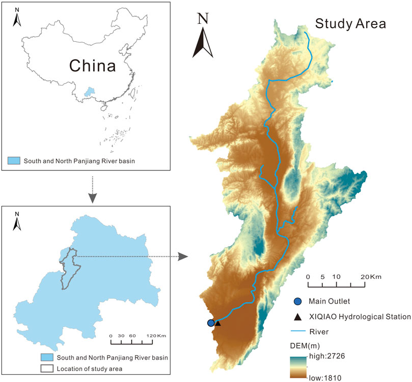
FIGURE 1. Location of the study area.
Digital elevation data (DEM) was acquired from the Geospatial Data Cloud (http://www.gscloud.cn/) with 30 m × 30 m resolution (Figure 1). It shows the spatial distribution of regional geomorphology. DEM data were used to analyze topography and slope, extract river network and sinkholes, make mask processing, and so on. Moreover, a watershed can be divided into multiple subbasins based on the river network and DEM in the SWAT model.
The land use map of the year 2015 was obtained from the Resource and Environment Science and Data Center Platform (http://www.resdc.cn/) with 1000 m resolution (Figure 2). We reclassified the initial land use map and got six land use types: farmland (AGRL), forest land (FRST), grassland (PAST), lakes and other bodies of water (WATR), urban construction land (URBN), and unused bare land (BALD). “AGRL,” “FRST,” and “PAST” are the three main land use types of the study area, and the areas are 823 km2 (30%), 778 km2 (28%), and 925 km2 (34%), respectively. The farmland near the river channel is mainly used for aquatic crops such as rice, and some irrigated farmland is used for crops such as corn and vegetables. Forestland types are mainly evergreen broad-leaved forest, deciduous broad-leaved forest, and coniferous forest. Grassland type is mainly natural grasslands with medium coverage.
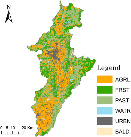
FIGURE 2. Classification of land cover types (year 2015).
Soil data were obtained from the Harmonized World Soil Database (HWSD) established by the United Nations Food and Agriculture Organization (FAO) and the International Institute for Applied Systems (IIASA) in Vienna, which linked to the soil characteristic database with a resolution of 1000 m × 1000 m. Each soil type contains physical and chemical properties. Thus, it plays an important role in the hydrological cycle in hydrological response units (HRUs) and affects the movement of water in the soil profile. We calculated the properties of the soil through the HWSD database, mathematical formula, and soil water characteristics module from SPAW software (Rao and Saxton 1995). The soil types which had the same soil names and properties were defined as the same one, and the final soil properties were made as a database in SWAT. mdb. The soil data were reclassified into 14 types as shown in Figure 3.
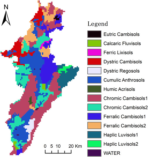
FIGURE 3. Classification of soil types.
The meteorological data used in the model were taken from The China Meteorological Assimilation Datasets for the SWAT model (CMADS) developed by Prof. Dr. Xianyong Meng (Meng and Wang 2017) from China Agricultural University (CAU). The CMADS data set has been modified as a format that the SWAT model can recognize and use the data set without any format conversion. The data include daily precipitation, maximum and minimum temperatures, solar radiation, relative humidity, and wind speed, from the year 2010 to 2015 at the 20 meteorological stations.
The calibration and verification data are the streamflow data of hydrological stations from the Institute of Karst Geology Chinese Academy of Geological Sciences. Average monthly streamflow data from the year 2012 to 2015 of the Xiqiao station from research institutes were used to calibrate the SWAT model. In addition, the daily streamflow data of the same station from 28 July 2015 to 4 October 2015 were also obtained. The location of the hydrological station mentioned previously is shown in Figure 1.
SWAT hydrological model simulation is divided into the overland flow phase and channel flow phase. The first phase controls the flow of water, sediment, and pollutants into the channel within the subbasin. The second phase is the process in which the flows from the first phase migrate to the outlet. The hydrologic processes simulated by the SWAT model mainly include surface runoff, soil infiltration, evapotranspiration, interflow, and return flow. The hydrology circulation system is based on the water balance equation (Arnold et al., 1998; HAO et al., 2006).
The aquifer constructed according to the regular SWAT model will be generalized as a loose homogeneous medium, and the infiltration delay days of soil profiles in karst areas are the same as in other areas in the traditional SWAT code. However, karst sinkholes have a phenomenon of rapid vertical replenishment, and the exchange rate of surface water and groundwater is much faster than that of other areas, which the regular model cannot accurately depict. In order to solve this problem, in this study, we used the pond module in SWAT to conceptualize the karst sinkholes and modified the algorithm to distinguish the rapid vertical replenishment hydrological process of the sinkholes.
Pond can receive a portion of the water from the subbasin, and its water storage is a function of daily inflow and outflow, including infiltration and evaporation. The outflow of the pond is simulated according to storage capacity and changes according to the soil moisture content and the flood season. The water balance equation of the pond in SWAT is shown in Formula (1):
where
The formula for controlling the pond hydrologic process in SWAT is as follows (Neitsch et al., 2002):
where
The pond module needs to be added at the subbasin scale, and all sinkholes are generalized with one pond for each subbasin. The pond was represented in the model by some specific parameter variables: a fraction of subbasin area that drains into ponds (PND_FR) and hydraulic conductivity through the bottom of ponds (PND_K). The parameters
In order to realize the change of water transfer speed and quantity in the vertical direction and rapid recharge of groundwater aquifer in sinkholes, we modified the original algorithm of the SWAT model. In the original model code (shown as Eq. 5), the amount of water from ponds (rchrgkarst) and percolation from the bottom of the soil profile in HRU [sepbtm(j)] use the same delay time variable which represents the duration of water leaving the bottom of the root zone to reach the shallow aquifer. With improvement, recharge is divided into two parts: leakage recharge of the soil profile and rapid recharge of karst sinkholes. The water passing through the pond was taken out separately, using a specific delay time variable. According to the empirical coefficient of previous models we built, the delay time variable of pond leakage was set to 1/50 of the initial value (as shown in Figure 4). After the modification of the SWAT code, the formula for calculating the daily recharge of the karst aquifer is given as Eq. 6:
where
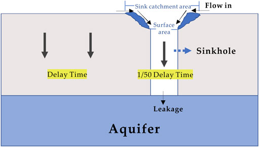
FIGURE 4. Karst sinkhole simulated by the pond module in the modified version of SWAT.
In the process of setting up the improved SWAT model, the DEM data were used to generate rivers and calculate the direction of flow. Then, the threshold value of the minimum area in the study catchment was set at 30000 Ha and generated the river network. Based on the river network and outlets, the study area was divided into five subbasins. The soil map and land use map were added to establish SWAT, and the corresponding index tables were imported to connect the map properties with the SWAT database. For slope classification, we selected the multiple slope method and divided slope into three levels: 0∼15, 15∼25, and 25∼9,999. After defining HRU and setting the minimum generative area ratio of land use, soil, and slope at 15, 15, and 10%, respectively, the SWAT model finally generated 833 HRUs (hydrological response units) in five subbasins.
We built two sets of models, which are called the original model and the improved model. No pond module was added to the original model, but in the improved model, we added the pond module to simulate karst sinkholes and the code of the pond was modified at the same time. In the improved model, the pond module was set in No. 1, No. 4, and No. 5 subbasins (as shown in Figure 5). Then, the surface area, initial volume, and volume of ponds when filled to spillway were, respectively, input into the model to complete the characterization of the pond.
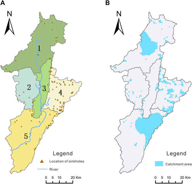
FIGURE 5. Division of watershed and location of sinkholes (A). Catchment area of the sinkholes in each subbasin (B).
In this study, we modified the SWAT source code in the Windows platform application development environment Visual Studio 2010. The subroutine gwmod. f was modified, and after modification and successful compilation, we replaced the original Swat. exe executable.
The SWAT model was calibrated using monthly streamflow data from 1 January 2012 to 31 December 2013 at Xiqiao stations in the study area. The Xiqiao Hydrological Station was chosen because the study area is an independent hydrogeological unit, and the Xiqiao Hydrological Station is located at the outlet of the whole basin. The warm up period was from 1 January 2010 to 31 December 2011. The validation period was from 1 January 2014 to 31 December 2015. During the simulation period, the maximum precipitation was 1171 mm, and the minimum precipitation was 402 mm, including the wet year and dry year. Model sensitivity analysis and calibration were carried out using the Sequential Uncertainty Fitting version 2 (SUFI-2) approach using the SWAT-CUP interface developed by Abbaspour (2015). Sensitivity analysis can determine the parameters that have a greater impact on the model and improve the simulation efficiency. The sensitivity of the parameter is determined by t factor and p factor, and the t factor is positively correlated with sensitivity, but p is negatively correlated. Model performance was evaluated based on statistical parameters of the coefficient of determination (R2) and Nash–Sutcliffe efficiency (NSE) (Moriasi et al., 2007). R2 and NSE are calculated as follows:
where
We used the hydrologic analysis tool in ArcGIS to identify negative terrain, calculate negative terrain depth, and generate catchment areas of the sinkholes. The field survey shows that the depth of sinkholes in the area is usually between 10 and 20 m, so we take negative terrain with this depth range as sinkholes. Because sinkholes are not only negative terrain but also have closed features, we identified contour lines and removed unclosed sinkholes. Figure 5 shows the location and catchment area of the sinkholes. In each subbasin, the area of all sinkholes was taken as the surface area of the pond and the average depth of all sinkholes was taken as the depth of the pond. The fraction of the subbasin area that drains into ponds (PND_FR) was the proportion of the catchment area of sinkholes to the subbasin area. Sinkhole parameters are shown in Table 1. It can be seen that the numbers of sinkholes in subbasins No. 2 and No. 3 are seven and five, respectively, and PND_FR is less than 0.05. It indicates that sinkholes are not widely distributed in these two subbasins compared with other subbasins. Therefore, the pond module was set in subbasins No. 1, No. 4, and No. 5. When extracting the river, a real river network map was added for guidance, and the “burn-in” algorithm in SWAT lowered the elevation of the river in DEM to generate a near-real river. The extracted river is shown in Figure 5.
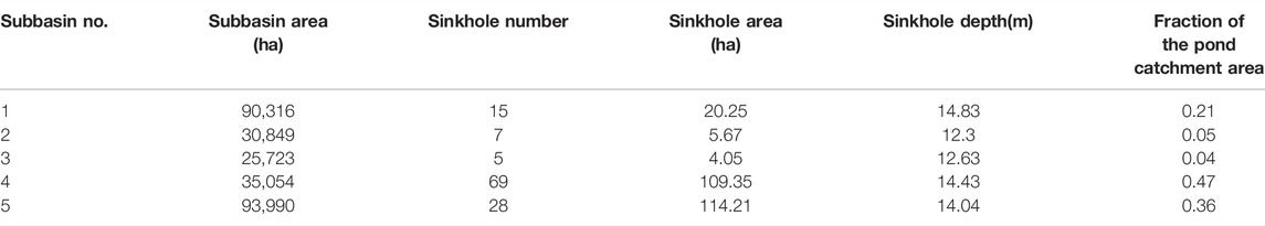
TABLE 1. Parameter characteristics of sinkholes in five subbasins.
During the calibration process, eight parameters were selected and 200 iterations were carried out in the hydrological stations. The parameter sensitivity, value ranges, and the final values are shown in Table.2, and rank stands for the sensitivity sequence. Soil conservation service curve number CN2 mainly affects surface runoff. Baseflow alpha factor ALPHA_BF affects the redistribution of groundwater runoff. Groundwater delay time GW_DELAY affects the groundwater delay. The three parameters are very sensitive, which is closely related to the hydrological process affected by a pond. Other parameters, such as the depth of water for return flow GWQMN, affect the generation of baseflow. The deep aquifer percolation fraction RCHRG_DP is the percolation fraction of the deep aquifer and describes the characteristics of the deep aquifer. The groundwater “revap” coefficient GW_REVAP and depth of water for evaporation REVAPMN affect the generation of baseflow by altering the evaporation of a shallow aquifer. PND_VOL affects the initial volume of the pond. All parameters were adjusted by replace, and the parameters identified in this study are consistent with those related studies (Moreira et al., 2018; Thavhana et al., 2018; Liang et al., 2020).
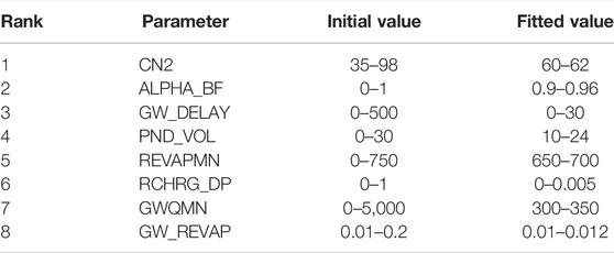
TABLE 2. Parameter sensitivity ranking and parameter fitted value range.
The streamflow data of the Xiqiao Hydrological Station were compared to assess the accuracy and applicability of the improved model (as shown in Figure 6). We used the same set of parameters before and after the model improvement, so that the change of the model only comes from the addition and improvement of the pond. The results show that for the original model, the value of R2 is 0.70 and NSE is 0.35 in the calibration period, while the value of R2 is 0.74 and NSE is 0.61 as simulated by the improved model. For the original model, R2 and NSE values are 0.76 and 0.66, respectively, in the validation period, while the value of R2 is 0.83 and NSE is 0.79 as obtained from the improved model. Both the linear correlation and model reliability have been strengthened with the improvements we proposed. In order to show the difference before and after improvement in more detail, we selected the flood season of the year 2015, July 28–October 4, and conducted daily simulation (as shown in Figure 7), and the result shows the decrease in peak flow and the increase in baseflow, especially in August, the simulated peak value and normal flow value are obviously closer to the measured data.
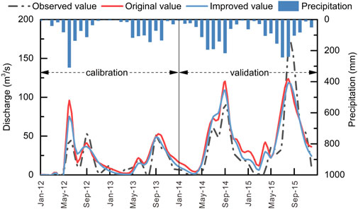
FIGURE 6. Monthly discharge during the calibration period (2012–2013) and the validation period (2014–2015) before and after model improvement.
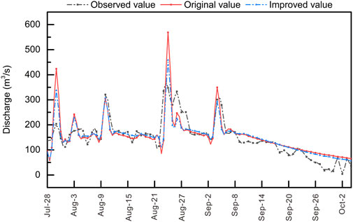
FIGURE 7. Daily discharge during the flood season in the year 2015 before and after model improvement.
According to the output. sub files obtained by the improved SWAT model, we calculated the average annual surface runoff depth and baseflow depth of No. 1, No. 4, and No. 5 subbasins. Compared with the improved model and original model (Table.3), the surface runoff depth was reduced by 9.2, 13.5, and 21.4 mm and the reduction rate was 21, 47, and 36%, respectively. Corresponding with the coefficient PND_FR that had been set in each subbasin, this result indicates that the subbasins with the pond let part of surface runoff flow into the pond, and the proportion of water flow in the pond was the value of the PND_FR parameter. Corresponding to the decrease in surface runoff, the baseflow depth of each subbasin increased. In the subbasins of No. 1, No. 4, and No. 5, the baseflow was increased by 16.4, 20.3, and 16.1 mm, respectively, which reflected the recharge of surface runoff to baseflow.
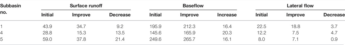
TABLE 3. Changes in surface runoff depth, baseflow depth, and lateral flow depth in the subbasins No. 1, No. 4, and No. 5 (unit: mm).
Compared with the original model, in the improved model, the lateral flow depth was reduced from 22.5 to 18.8 mm in subbasin No. 1, from 12.2 to 7.5 mm in subbasin No. 4, and 8.0 to 7.1 mm in subbasin No. 5. The water yield is composed of surface runoff, baseflow, and lateral flow. In the original model, the water yield of subbasins No. 1, No. 4, and No. 5 was 262.4, 186.6, and 316.6 mm, respectively, and the total water yield was 765.6 mm. In the improved model, the water yield of subbasins No. 1, No. 4, and No. 5 was 265.8, 188.7, and 310.6 mm, respectively, and the total water yield was 765.1 mm. The water yield was basically under a state of water balance. It can be seen that the recharge of surface runoff to baseflow caused a decrease in lateral flow, and a part of the lateral flow was directly converted into the baseflow to recharge the river.
According to the results of SWAT, we analyzed the spatial distribution of river discharge, runoff modulus, surface runoff depth, and baseflow depth. Figure 8 shows that the rivers in the subbasins No. 1, No. 2, and No. 4 are located in the upstream and tributaries, and the annual average discharge is 7.2 m3/s, 8.4 m3/s, and 6.8 m3/s, respectively. The rivers in subbasins No. 3 and No. 5 are located in the downstream and the mainstream, and the annual average discharge is 19.0 m3/s and 33.6 m3/s, respectively. The discharge of the river shows the distribution characteristics of increasing gradually from upstream to downstream and from tributaries to mainstreams.
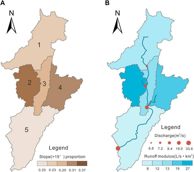
FIGURE 8. Spatial distribution of slope (>15°) proportion (A). Spatial distribution of river discharge and runoff modulus (B).
A runoff modulus is a basic hydrogeological parameter, which can compare runoff in different subbasins. The slope is a land feature, and the slope above 15° is classified as a steep slope. We calculated the runoff modulus and the proportion of slope above 15° for each subbasin (as shown in Figure 8). In subbasin No. 2, the runoff modulus is 27 L/s·km2, the slope ratio is 0.37, and both the parameters are the largest. In subbasin No. 5, the runoff modulus is 8 L/s·km2, the slope ratio is 0.20, and both the parameters are the smallest. Comparing the runoff modulus with the slope distribution in Figure 8, the larger the proportion of steep slopes, the larger the runoff modulus. As the slope increases, the velocity of surface runoff becomes faster, the duration of runoff generation on the slope is short, and the infiltration amount is small. On the contrary, the runoff is large.
The distribution of hydrological components is influenced by land use. The land use types are mainly farmland (AGRL), forest land (FRST), and grassland (PAST) in the study area. The surface runoff depth and baseflow depth generated by these three land use types in each subbasin were calculated. Figure 9 shows that for surface runoff depth, AGRL > FRST > PAST. However, Figure 10 shows that for baseflow depth, FRST > PAST > AGRL. It can be seen that the surface runoff and baseflow are related to the land use types. Farmland is more likely to produce surface runoff, and forest land produces more baseflow due to water conservation of vegetation. The root system of crops is underdeveloped and cannot consolidate the soil well. The surface runoff will wash the surface soil of farmland and generate more runoff. The phenomenon of soil physical crusting often occurs on the surface of overcultivated land, which will also increase the runoff. The forest root system is very developed, and forest soil has a good structure and porosity; so the infiltration velocity is fast, which plays the role of intercepting surface runoff and generating baseflow.
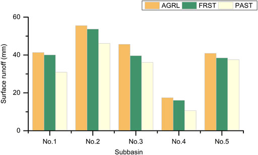
FIGURE 9. Average annual surface runoff depth in each subbasin under different land use types.
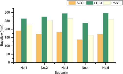
FIGURE 10. Average annual baseflow depth in each subbasin under different land use types.
For the traditional hydrological process, streamflow is the sum of surface flow, lateral flow, and baseflow, but in our study area, the unique karst topography differentiates the process and a part of water enters the deep aquifer through high-permeability channels and forms preferential flow (Rimmer and Salingar 2006). Using the model to accurately show the surface runoff and baseflow in karst areas is useful for analyzing the quick and large response of groundwater discharge to rainfall events, karst underground floods, the transport of sediment, and organic material.
In this study, we used the pond module in SWAT to simulate sinkholes. After improvement, the indicators of NSE and R2 have been strengthened in the 2012–2015 monthly scale simulation. In the improved model, the simulated flow line is closer to the observed data, especially the decrease can be observed at the peak value of the surface runoff at the Xiqiao Hydrological Station. For subbasins No. 1, No. 4, and No. 5, the surface runoff was relatively decreased and baseflow was relatively increased after improvement. This change was due to the addition of the pond module, which made a part of surface water to quickly replenish groundwater through karst sinkholes. Moreover, in the steady stage of the flood season, the flow process line rises, which reflects that the baseline was elevated. It can be concluded that the addition of pond module and characterization of karst morphology will change the amount of surface water and groundwater resource allocation in the modified subbasin, the flow distribution between surface runoff and baseflow was changed, and the improved model outperformed the original model in terms of both the model fitting effect and model quality and enabled to simulate the recharge process and the hydrologic cycle of the sinkholes.
During the simulation, R2 and NSE in the validation period were better than the calibration period because R2 and NSE are sensitive to the peak value of river discharge. However, the simulated peak value in June 2012 was much greater than the observed value. Although the improved model weakened the surface runoff, it still overpredicted this value, so R2 and NSE in the calibration period are smaller than the validation period. The reason for this phenomenon is the heavy rainfall in June 2012, which reached 325 mm. The SWAT model is sensitive to rainfall, and the simulated curve reflects this peak value of discharge caused by heavy rainfall. But, before six months, this heavy rainfall is the dry season, with an average of only 22 mm of rainfall per month. The heavy rainfall recharged the soil water and karst fissures first so that the observed value did not show a peak value of discharge.
The karst area simulation is still in the exploration stage, especially the application results of the SWAT model to depict karst morphology are not abundant. In Southwest China, some scholars exposed the karst underground river to the surface and some scholars generated HRUs according to karst characteristics, but these studies did not involve the hydrologic process of sinkholes (Yu et al., 2012; Zhang et al., 2020). Outside of Southwest China, Palanisamy and Workman, (2014) proposed KarstSWAT to simulate sinkholes located on the streambed in the Cane Run watershed. They simulated the horizontal hydrologic process of flow from the stream channel into the deep aquifer through sinkholes and then transferred from karst conduits to spring. But in our study, sinkholes are located all over the watershed, and we focused on the vertical hydrologic process of sinkholes rapidly diverting the surface water to the shallow aquifer through large hydraulic conductivity and short delay time. We used the pond module in SWAT to simulate sinkholes as same as Baffaut and Benson, (2009), and their study specifically analyzed the flow simulation characteristic of the improved SWAT model in southwest Missouri. In our study, we further defined a specific value of delay time in the pond and compared the quantity changes of hydrology components surface runoff depth and baseflow depth before and after improvement and analyzed the water balance relationship. This method is suitable for any karst area with sinkholes because the area and volume of sinkholes can be obtained by remote sensing interpretation or field investigation in any study area, and the pond module can generalize the sinkhole characteristics and describe the vertical connection between the surface and underground. We successfully simulated sinkholes in Southwest China, which also proved that this method can be applied to karst landscapes in different regions. In addition, field investigation of karst sinkholes is an arduous task (Bakalowicz 2005; Zisman et al., 2013). We applied the sinkhole parameters analyzed by DEM to the model and obtained good results, which provided a method for the simulation of karst areas with few field investigation data. We aimed at the source area of the South Panjiang River in this study. It is necessary to further analyze the distribution situation of the sinkholes in the whole SNPB and popularize this method to describe the karst characteristic in more detail.
In this study, we conceptualized the sinkholes as the pond with large hydraulic conductivity at the bottom, and the fast recharge response of karst was realized by modifying the groundwater delay time of the algorithm with the SWAT model. The improved model was fitted with the measured data of the Xiqiao Hydrological Station, and it was verified that R2 and NSE can achieve satisfactory results. The surface runoff of karst subbasins No. 1, No. 4, and No. 5 with the pond module was significantly decreased by 21, 47, and 36% corresponding to the PND_FR values 0.21, 0.47, and 0.36, respectively. The baseflow of the subbasins was increased significantly, and the pond module also made a portion of lateral flow become baseflow. After the improvement, the evaluation factor R2 of the Xiqiao station increased from 0.70 to 0.74 and NSE increased from 0.35 to 0.61 during the calibration period. In the validation period, the R2 increased from 0.76 to 0.83 and NSE increased from 0.66 to 0.79. Using the improved model to explore the spatial distribution of hydrological components, it was found the runoff modulus in the study area has a positive correlation related to the slope (>15°) proportion, the baseflow depth and surface runoff depth are related to the land use types, farmland produces more surface runoff, and forest land produces more baseflow. This study proved that the improved model simulates sinkholes successfully and has a better effect than the original model. This method can describe the preferential flow of the karst sinkhole and the reallocation of surface water and groundwater.
The original contributions presented in the study are included in the article/supplementary material, further inquiries can be directed to the corresponding author.
YZ: drafting the manuscript. LZ: supervision and data curation. JC: investigation and data collection of the study area. YW: creation of models.
This study was supported by the “Study on nonlinear Features of Water Exchange between Conduit and Matrix in Karst dual Water-bearing Medium” from “The National Science Fund for Distinguished Young Scholars” (42102296).
YW was employed by the company Hebei Hydrological Engineering Geological Survey Institute Co, Ltd.
The remaining authors declare that the research was conducted in the absence of any commercial or financial relationships that could be construed as a potential conflict of interest.
All claims expressed in this article are solely those of the authors and do not necessarily represent those of their affiliated organizations, or those of the publisher, the editors, and the reviewers. Any product that may be evaluated in this article, or claim that may be made by its manufacturer, is not guaranteed or endorsed by the publisher.
Abbaspour, K. C. (2015). SWAT-CUP: SWAT Calibration and Uncertainty Programs. Switzerland: EAWAG: Dübendorf, 130.
Anand, J., Gosain, A. K., and Khosa, R. (2018). Prediction of Land Use Changes Based on Land Change Modeler and Attribution of Changes in the Water Balance of Ganga Basin to Land Use Change Using the SWAT Model. Sci. Total Environ. 644 (dec.10), 503–519. doi:10.1016/j.scitotenv.2018.07.017
Arnold, J. G., Srinivasan, R., Muttiah, R. S., and Williams, J. R. (1998). Large Area Hydrologic Modeling and Assessment Part I: Model Development. JAWRA J. Am. Water Resour. Assoc. 34 (1), 1–17. doi:10.1111/j.1752-1688.1998.tb05961.x
Bakalowicz, M. (2005). Karst Groundwater: a Challenge for New Resources. Hydrogeol. J. 13 (1), 148–160. doi:10.1007/s10040-004-0402-9
Baker, T. J., and Miller, S. N. (2013). Using the Soil and Water Assessment Tool (SWAT) to Assess Land Use Impact on Water Resources in an East African Watershed. J. Hydrology 486, 100–111. doi:10.1016/j.jhydrol.2013.01.041
Cahalan, M. D., and Milewski, A. M. (2015). Sinkhole Formation Mechanisms and Geostatistical-Based Prediction Analysis in a Mantled Karst Terrain. Catena 165, 333–344.
C. Baffaut, C., and V. W. Benson, V. W. (2009). Modeling Flow and Pollutant Transport in a Karst Watershed with SWAT. Trans. ASABE 52 (2), 469–479. doi:10.13031/2013.26840
Deni-Juki, V., and Juki, D. (2003). Composite Transfer Functions for Karst Aquifers. J. Hydrology 274 (1-4), 0–94.
D. M. Amatya, D. M., M. Jha, M., A. E. Edwards, A. E., D. R. Hitchcock, T. M., and Hitchcock, D. R. (2011). Swat-Based Streamflow and Embayment Modeling of Karst-Affected Chapel Branch Watershed, South Carolina. Trans. Asabe 54 (4), 1311–1323. doi:10.13031/2013.39033
D. N. Moriasi, D. N., J. G. Arnold, J. G., M. W. Van Liew, M. W. V., R. L. Bingner, R. L., T. L. Veith, R. D., and Veith, T. L. (2007). Model Evaluation Guidelines for Systematic Quantification of Accuracy in Watershed Simulations. Trans. Asabe 50 (3), 885–900. doi:10.13031/2013.23153
Felton, G. K., and Currens, J. C. (1994). Peak Flow Rate and Recession-Curve Characteristics of a Karst Spring in the Inner Bluegrass, Central Kentucky. J. Hydrology 162 (1–2), 99–118. doi:10.1016/0022-1694(94)90006-x
Ford, D., and Williams, P. (2007). Karst Hydrogeology and Geomorphology. American Geophysical Union.
Halihan, T., and Wicks, C. M. (1998). Modeling of Storm Responses in Conduit Flow Aquifers with Reservoirs. J. Hydrology 208 (1-2), 82–91. doi:10.1016/s0022-1694(98)00149-8
Hao, F. H., Cheng, H. G., and Yang, S. T. (2006). Non-point Source Pollution Model. Beijing: China Environ Science Press.
Hartmann, A., Goldscheider, N., Wagener, T., Lange, J., and Weiler, M. (2014). Karst Water Resources in a Changing World: Review of Hydrological Modeling Approaches. Rev. Geophys. 52 (No.3), 218–242. doi:10.1002/2013rg000443
Hartmann, A., Lange, J., Weiler, M., Arbel, Y., and Greenbaum, N. (2012). A New Approach to Model the Spatial and Temporal Variability of Recharge to Karst Aquifers. Hydrology Earth Syst. Sci. 16 (No.7), 2219–2231. doi:10.5194/hess-16-2219-2012
Hu, C., Hao, Y., Yeh, T.-C. J., Pang, B., and Wu, Z. (2008). Simulation of Spring Flows from a Karst Aquifer with an Artificial Neural Network. Hydrol. Process. 22 (5), 596–604. doi:10.1002/hyp.6625
Huang, Z., Yeh, P. J.-F., Pan, Y., Jiao, J. J., Gong, H., Li, X., et al. (2019). Detection of Large-Scale Groundwater Storage Variability over the Karstic Regions in Southwest China. J. Hydrology 569, 409–422. doi:10.1016/j.jhydrol.2018.11.071
Lallahem, S., Mania, J., Hani, A., and Najjar, Y. (2005). On the Use of Neural Networks to Evaluate Groundwater Levels in Fractured Media. J. Hydrology 307 (1-4), 92–111. doi:10.1016/j.jhydrol.2004.10.005
Lauber, U., Ufrecht, W., and Goldscheider, N. (2014). Spatially Resolved Information on Karst Conduit Flow from In-Cave Dye-Tracing. Hydrology Earth Syst. Sci. Discuss. 10 (9), 11311–11335. doi:10.5194/hess-18-435-2014
Li, G., Rubinato, M., Wan, L., Wu, B., Fang, J. J., and Zhou, J. (2020). Preliminary Characterization of Underground Hydrological Processes under Multiple Rainfall Conditions and Rocky Desertification Degrees in Karst Regions of Southwest China. Water 12 (2), 594. doi:10.3390/w12020594
Liang, G., Qin, X., Cui, Y., Chen, S., and Huang, Q. (2020). Improvement and Application of a Distributed Hydrological Model in Karst Regions. Hydrogeology Eng. Geol. 47 (2), 60–67.
Liu, J., Ding, H., Xiao, M., Xu, Z.-Y., Su, Y. Z.-H., Zhao, L., et al. (2020). Climatic Variabilities Control the Solute Dynamics of Monsoon Karstic River: Approaches from C-Q Relationship, Isotopes, and Model Analysis in the Liujiang River. Water 12 (3), 862. doi:10.3390/w12030862
Makropoulos, C., Koutsoyiannis, D., Stanić, M., Djordjević, S., Prodanović, D., Dašić, T., et al. (2008). A Multi-Model Approach to the Simulation of Large Scale Karst Flows. J. Hydrology 348 (3–4). doi:10.1016/j.jhydrol.2007.10.011
Malagò, A., Efstathiou, D., Bouraoui, F., Nikolaidis, N. P., Franchini, M., Bidoglio, G., et al. (2016). Regional Scale Hydrologic Modeling of a Karst-Dominant Geomorphology: The Case Study of the Island of Crete. J. Hydrology 540, 64–81.
Martínez-Salvador, A., and Conesa-García, C. (2020). Suitability of the SWAT Model for Simulating Water Discharge and Sediment Load in a Karst Watershed of the Semiarid Mediterranean Basin. Water Resour. Manag. 34 (2), 785–802.
Martínez-Santos, P., and Andreu, J. M. (2010). Lumped and Distributed Approaches to Model Natural Recharge in Semiarid Karst Aquifers. J. Hydrology 388 (3), 389–398.
Meng, H., and Wang, L. (2010). Advance in Karst Hydrological Model. Prog. Geogr. 29 (11), 1311–1318.
Meng, X. Y., and Wang, H. (2017). Significance of the China Meteorological Assimilation Driving Datasets for the SWAT Model (CMADS) of East Asia. Water 9 (10), 5. doi:10.3390/w9100765
Moreira, L. L., Schwamback, D., and Rigo, D. (2018). Sensitivity Analysis of the Soil and Water Assessment Tools (SWAT) Model in Streamflow Modeling in a Rural River Basin. Revista Ambiente Água 13 (6), e2221. doi:10.4136/ambi-agua.2221
Neitsch, S. L., Arnold, J. G., Kiniry, J. R., Williams, J. R., and King, K. W. (2002). Soil and Water Assessment Tool Theoretical Documentation. version 2000.
Nhu, V. H., Rahmati, O., Falah, F., Shojaei, S., Al-Ansari, N., Shahabi, H., et al. (2020). Mapping of Groundwater Spring Potential in Karst Aquifer System Using Novel Ensemble Bivariate and Multivariate Models. Water 12 (4), 25. doi:10.3390/w12040985
Nie, W., Yuan, Y., Kepner, W., Nash, M. S., Jackson, M., and Erickson, C. (2011). Assessing Impacts of Landuse and Landcover Changes on Hydrology for the Upper San Pedro Watershed. J. Hydrology 407 (1-4), 105–114. doi:10.1016/j.jhydrol.2011.07.012
Palanisamy, B., and Workman, S. R. (2014). Hydrologic Modeling of Flow through Sinkholes Located in Streambeds of Cane Run Stream, Kentucky. J. Hydrologic Eng. 20 (5), 04014066.
Piniewski, M., Bieger, K., and Mehdi, B. (2019). Advancements in Soil and Water Assessment Tool (SWAT) for Ecohydrological Modelling and Application. Ecohydrol. Hydrobiology 19, 179–181. doi:10.1016/j.ecohyd.2019.05.001
Rahman, M. M., Thompson, J. R., and Flower, R. J. (2016). An Enhanced SWAT Wetland Module to Quantify Hydraulic Interactions between Riparian Depressional Wetlands, Rivers and Aquifers. Environ. Model. Softw. 84, 263–289. doi:10.1016/j.envsoft.2016.07.003
Rao, A. S., and Saxton, K. E. (1995). Analysis of Soil Water and Water Stress for Pearl Millet in an Indian Arid Region Using the SPAW Model. J. Arid Environ. 29 (2), 155–167. doi:10.1016/s0140-1963(05)80086-2
Rimmer, A., and Salingar, Y. (2006). Modelling Precipitation-Streamflow Processes in Karst Basin: The Case of the Jordan River Sources, Israel. J. Hydrology 331 (3-4), 524–542. doi:10.1016/j.jhydrol.2006.06.003
Salerno, F., and Tartari, G. (2009). A Coupled Approach of Surface Hydrological Modelling and Wavelet Analysis for Understanding the Baseflow Components of River Discharge in Karst Environments. J. Hydrology 376 (1–2), 295–306. doi:10.1016/j.jhydrol.2009.07.042
Samuels, R., Rimmer, A., Hartmann, A., Krichak, S., and Alpert, P. (2010). Climate Change Impacts on Jordan River Flow: Downscaling Application from a Regional Climate Model. J. Hydrometeorol. 11 (4), 860–879. doi:10.1175/2010jhm1177.1
Schomberg, J. D., Host, G., Johnson, L. B., and Richards, C. (2005). Evaluating the Influence of Landform, Surficial Geology, and Land Use on Streams Using Hydrologic Simulation Modeling. Aquat. Sci. 67 (4), 528–540. doi:10.1007/s00027-005-0785-2
Sezen, C., Bezak, N., Bai, Y., and Šraj, M. (2019). Hydrological Modelling of Karst Catchment Using Lumped Conceptual and Data Mining Models. J. Hydrology 576, 98–110. doi:10.1016/j.jhydrol.2019.06.036
Shang, X., Jiang, X., Jia, R., and Wei, C. (2019). Land Use and Climate Change Effects on Surface Runoff Variations in the Upper Heihe River Basin. Water 11 (2), 344. doi:10.3390/w11020344
Thavhana, M. P., Savage, M. J., and Moeletsi, M. E. (2018). SWAT Model Uncertainty Analysis, Calibration and Validation for Runoff Simulation in the Luvuvhu River Catchment, South Africa. Phys. Chem. Earth, Parts A/B/C 105, 115–124. doi:10.1016/j.pce.2018.03.012
Villamizar, S. R., Pineda, S. M., and Carrillo, G. A. (2019). The Effects of Land Use and Climate Change on the Water Yield of a Watershed in Colombia. Water 11 (2), 285. doi:10.3390/w11020285
Valdes-Abellan, J., Pla, C., Fernandez-Mejuto, M., and Andreu, J. M. (2018). Validating the KAGIS Black-Box GIS-Based Model in a Mediterranean Karst Aquifer: Case of Study of Mela Aquifer (SE Spain). Hydrol. Process. 32 (16), 2584–2596. doi:10.1002/hyp.13215
Veress, M. (2020). Karst Types and Their Karstification. J. Earth Sci. 31 (3), 621–634. doi:10.1007/s12583-020-1306-x
Wang, Y., Shao, J., Su, C., Cui, Y., and Zhang, Q. (2019). The Application of Improved SWAT Model to Hydrological Cycle Study in Karst Area of South China. Sustainability 11 (18), 5024. doi:10.3390/su11185024
Xie, K., Chen, H., Qiu, Y., Kim, J.-S., Yoon, S.-K., Lin, Y., et al. (2021). Exploring and Predicting the Individual, Combined, and Synergistic Impact of Land-Use Change and Climate Change on Streamflow, Sediment, and Total Phosphorus Loads. Front. Environ. Sci. 9, 726793. doi:10.3389/fenvs.2021.726793
Yu, D., Sun, L., Yu, J., and Wang, Z. (2012). Simulation on Soil Erosion and Streamflow in Maotiaohe Watershed of Guizhou Province Based on SWAT Model. Chin. Agric. Sci. Bull. 28 (17), 256–261.
Zhang, C., Zhang, F., Geng, X., Ji, J., and Chen, Y. (2020). Generalization Method of Karst Underground River in SWAT:An Example of the Daotian River Watershed in Bijie, Guizhou. Carsologica Sin. 39 (5), 665–672.
Zhou, S., Zhang, W., and Guo, Y. (2020). Impacts of Climate and Land-Use Changes on the Hydrological Processes in the Amur River Basin. Water 12 (1), 76.
Keywords: karst area, sinkhole, semi-distributed model SWAT, surface runoff, baseflow
Citation: Zhou Y, Zhao L, Cao J and Wang Y (2022) Using an Improved SWAT Model to Simulate Karst Sinkholes: A Case Study in Southwest China. Front. Environ. Sci. 10:950098. doi: 10.3389/fenvs.2022.950098
Received: 22 May 2022; Accepted: 22 June 2022;
Published: 22 July 2022.
Edited by:
Yong Xiao, Southwest Jiaotong University, ChinaReviewed by:
Zhonghua Tang, China University of Geosciences, ChinaCopyright © 2022 Zhou, Zhao, Cao and Wang. This is an open-access article distributed under the terms of the Creative Commons Attribution License (CC BY). The use, distribution or reproduction in other forums is permitted, provided the original author(s) and the copyright owner(s) are credited and that the original publication in this journal is cited, in accordance with accepted academic practice. No use, distribution or reproduction is permitted which does not comply with these terms.
*Correspondence: Liangjie Zhao, emhhb2xpYW5namllQG1haWwuY2dzLmdvdi5jbg==
Disclaimer: All claims expressed in this article are solely those of the authors and do not necessarily represent those of their affiliated organizations, or those of the publisher, the editors and the reviewers. Any product that may be evaluated in this article or claim that may be made by its manufacturer is not guaranteed or endorsed by the publisher.
Research integrity at Frontiers
Learn more about the work of our research integrity team to safeguard the quality of each article we publish.