The Statistical Characteristics of Atmospheric Ducts Observed Over Stations in Different Regions of American Mainland Based on High-Resolution GPS Radiosonde Soundings

Atmospheric duct is an anomalous atmospheric structure that affects electromagnetic wave propagation. The important characteristics of the atmospheric ducts include duct probability, duct height, duct strength, and the thickness of the trapping layer. To investigate the statistical characteristics of atmospheric ducts over the American mainland, four stations in different regions are chosen. The seasonal and diurnal variation of the characteristics of ducts is presented. The mechanism of the seasonal and variation of ducts is revealed and the relationship between the characteristics is researched. The duct strength correlates positively with the thickness of the trapping layer, and the duct height correlates with them negatively. Moreover, the duct relationship with precipitation over different stations is clarified. It is found that the precipitation correlates positively with the probability of ducts caused by the vertical moisture gradient, and the relation is negative when the ducts are caused by temperature inversion. This work is of great value to the statistical characteristics of atmospheric ducts over the American mainland.

Introduction

Electromagnetic wave (EMW) propagation is often affected in the atmosphere. They may be absorbed, reflected, and trapped due to the inhomogeneous atmospheric refractive index. Among these phenomena, the phenomenon that EMW is trapped in a specific layer is very important and is named the atmospheric duct. The phenomenon is caused by the gradient in refractivity with regard to altitude. Many meteorological processes are associated with it, like temperature inversion, moisture inversion, the subsidence of air masses, and the passing of cold air over warm land (Manjula et al., 2016).

The atmospheric duct can be observed frequently over the sea surface and the coastal areas where the humidity decreases rapidly with the altitude. All ducts can be divided into three categories: surface ducts, elevated ducts, and evaporation ducts. There are many different ways to determine the ducts based on their different features. For the evaporation duct, the diagnosis models are employed to evaluate the evaporation duct height. The refractivity from radar clutter (RFC) technique is also used to calculate the ducting profiles (Rogers et al., 2000; Yardim et al., 2008; Karimian et al., 2011). In recent years, there are many research studies which calculated the ducts based on machine learning methods (Yan et al., 2018; Zhu et al., 2018; Han et al., 2021; Zhao et al., 2021). For the surface ducts, the RFC technique also works. However, the RFC accuracy still needs to be improved, and this technique cannot be used in elevated and some surface-based ducts (Karimian et al., 2011). As a result, to determine the two ducts, the most common method is to use Global Positioning System (GPS) radiosondes to measure meteorological parameters and then indirectly calculate the profiles (Ding et al., 2013; Li et al., 2021). Moreover, the use of refractometers to directly measure the atmospheric refractivity at a vertical height is feasible.

Since the atmospheric duct is of great value to radar detection and radio communication, there have been numerous studies on the characteristics and variation of atmospheric ducts (Haack and Burk, 2001; Ding et al., 2013; Mai et al., 2020). Von Engeln. (2004) analyzed the characteristics of global atmospheric ducts using reanalysis data from the European Centre for Medium-Range Weather Forecasts (ECMWF). Sirkova (2015) performed a research on the duct occurrence and the spatial–temporal distribution in the Bulgarian Black Sea shore, and the essential duct parameters for surface and elevated ducts are reported for summer months. Moreover, the GPS radiosondes measuring the meteorological parameters, including temperature, pressure, and humidity, are used to determine the vertical refractivity profiles. Sun et al. (2016) used high-resolution radiosondes to first observe the elevated ducts associated with intermittent turbulence over the Bosten Lake and explained the mechanism well. Li et al. (2021) presented the distribution of clouds and the elevated ducts over the central Western Pacific Ocean using GPS data and Himawari-8 satellite products. It is discovered that the appearance of low clouds can lead to a strong temperature and humidity inversion, which makes the elevated ducts stronger.

This article will study the statistical characteristics of ducts over stations in different regions of America based on the Stratosphere-Troposphere Process and their Role in Climate (SPARC) high-resolution radiosonde data at universal time (UT)00 and UT12 in a day for over 10 years. First, the seasonal and diurnal variation of the relative humidity (RH) and temperature is shown. Second, the seasonal variation of ducting probability, altitude, strength, and ducting thickness of each station are presented and the mechanism is revealed. Next, the diurnal variation of the characteristics is researched and the reason for this variation is proposed. The total precipitation associated with ducting is researched by comparing the ducting conditions with the total precipitation in different regions and seasons.

Materials and Methods

RRS Radiosonde Data, SRTM15 Elevation Data, and ERA-5 Reanalysis Data

In this work, high-resolution radiosonde data are obtained from the Radiosonde Replacement System (RRS) from NOAA’s National Centers for Environmental Information at 1-s temporal resolution for all stations from 2005 to 2019. The observation time is at 0 and 12 in 1 day and the vertical resolution is about 5–10 m. The maximum height we consider is 5 km because of the conclusion obtained by Kursinski et al. (2000). The radiosondes measure different meteorological parameters, including temperature (T), relative humidity (RH), and pressure (P) at each specific altitude. Then, these parameters are used to calculate the refractivity profiles. There are hundreds of stations over the American mainland, and to be representative, four stations from the northwest, middle, southwest, and southeast of America were chosen to be investigated. They are chosen for they can typically represent different climates of America, which vary in humidity and temperature. Specifically, Albany belongs to the humid continental climate and Dodge City belongs to the semiarid steppe climate. Boise belongs to the alpine climate and Charles belongs to the subtropical monsoon climate. By figuring out the statistics of the ducts over the stations, the overall ducting characteristics of America will be more obvious. The basic information and the number of sondes available in the stations are, respectively, presented in Table 1. The general geographical locations of them are shown in Figure 1.

TABLE 1

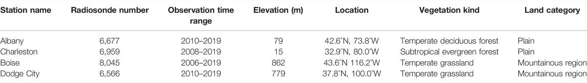
TABLE 1. Basic information of the four stations. The station number is in the format from Weather Bureau, Air Force, and Navy (WBAN).

FIGURE 1

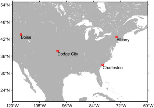
FIGURE 1. Locations of the four stations are marked with red hollow circles in American mainland.

Second, the elevation data used in this work are SRTM15 Digital Elevation Model (DEM) from the National Aeronautics and Space Administration (NASA) and the National Bureau of Image and Mapping (NIMA). The horizonal resolution of the data is 450 m, and the coverage area is global land. The data are used because the calculation of the refractivity profiles needs the elevation when the Earth’s curvature is taken into consideration.

Finally, the reanalysis data utilized are from the ERA-5 reanalysis dataset from the European Centre for Medium-Range Weather Forecasts (ECWMF). The spatial resolution of the dataset is 0.25° × 0.25° and the temporal resolution is 1 h. The time range in this work is 2010–2019. Sixteen pressure levels, namely, 500, 550, 600, 650, 700, 750, 775, 800, 825, 850, 875, 900, 925, 950, 975, and 1000 hPa are selected to obtain the vertical variations. To research the meteorological parameters over the four stations, four grids $\left({42.75}^{\circ }N,{74}^{\circ }W\right),\left({33}^{\circ }N,{80}^{\circ }W\right),\left({43.75}^{\circ }N,{116.25}^{\circ }W\right),\text{ and }\left({38}^{\circ }N,{100}^{\circ }W\right)$ are chosen to analyze the differences between their duct characteristics. The variables used here are relative humidity, temperature, and precipitation.

Methods of Calculating Refractivity Profiles and Quality Control

The formula for calculating refractivity was put forward by Smith and Weintraub (1953). It is as follows:

$N=\frac{77.6p}{T}-\frac{5.6e}{T}+\frac{3.75\times {10}^{5}e}{T^2},(1)$

$e=RH\ast e_s,(2)$

where $T$ (K) is the absolute temperature, $e$ (hPa) is the water vapor pressure, $e_s$ (hPa) is the saturated vapor pressure of water, and $p$ (hPa) is the atmospheric pressure. The formula of $e_s$ is as follows (Bolton, 1980):

$e_s\left(t\right)=6.112\ast \exp \left(\frac{17.67t}{t+243.5}\right),(3)$

where $t$ (°C) is the temperature in centigrade. After taking the Earth’s curvature into consideration, the modified refractivity (M) is defined by the empirical equation (Babin and Rowland, 1992):

$M=N+\frac{z}{{10}^{-6}{a}_e},(4)$

where $z$ (m) is the altitude above the Earth’s surface and $a_e$ (m) is the local radius of the Earth. Using the measured temperature, relative humidity, atmospheric pressure at different heights, and the local elevation of the station, the refractivity profiles are calculated.

Before determining atmospheric ducts, the quality control of data is necessary. First, we examine the temperature, relative humidity, and pressure profiles for the abnormal data points in them because of the errors of the radiosondes. The values of the points are replaced by the average of the surrounding points if they are judged to be abnormal. Second, the raw refractivity profiles are gridded to 50 m to remove outliers caused by the random motion of the radiosondes. $M$ increases with the increase in the height, and when the atmospheric ducts occur, $M$ decreases with the increase in the height. As a result, the ducts can be determined by

$\frac{dM}{dz}<0.(5)$

The altitude at which the gradient of $M$ turns negative is the duct height. The thickness of the trapping layer is defined as the distance between the top of the ducting layer and the height with the maximum value of $M$ in the ducting layer. The duct strength is defined as the difference between the maximum and the minimum value of $M$ in the ducting layer. Finally, to identify effective ducting layers, potential ducting layers whose duct strength is greater than 2 M can be regarded as real ducting layers. The above characteristics of the three types of ducts are shown in Figure 2. Combining with the above three procedures, the noise resulting from the measurement is eliminated and the effective ducting layers are obtained. In addition, the characteristics of the ducting layer with the maximum strength in a multiple-layer duct are regarded as the characteristics of the entire duct.

FIGURE 2

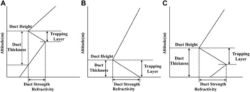
FIGURE 2. Vertical refractivity profiles of surface ducts (A), surface-based ducts (B), and elevated ducts (C), and the characteristics of them.

Seasonal and Diurnal Variations of Relative Humidity and Temperature

To investigate the characteristics of the ducts over the four stations, the meteorological parameters over them are first presented. The ducts are affected mostly by the moisture and the temperature vertical gradient, the seasonal (Figure 3) and diurnal (Figure 4) variation of the relative humidity (RH), and temperature at different pressure levels. The RH and temperature data are from the ERA-5 reanalysis dataset.

FIGURE 3

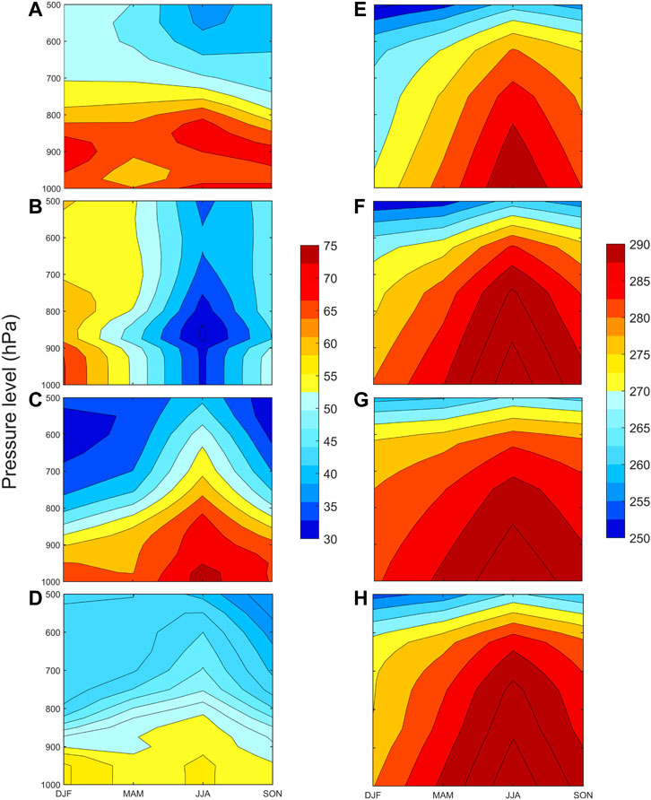
FIGURE 3. Variation of relative humidity (A–D) (unit: %) and temperature (E–H) (unit: K) with altitude and seasons. (A) (E) Situation in Albany. (B) (F) Situation in Boise. (C) (G) Situation in Charleston. (D) (H) Situation in Dodge City.

FIGURE 4

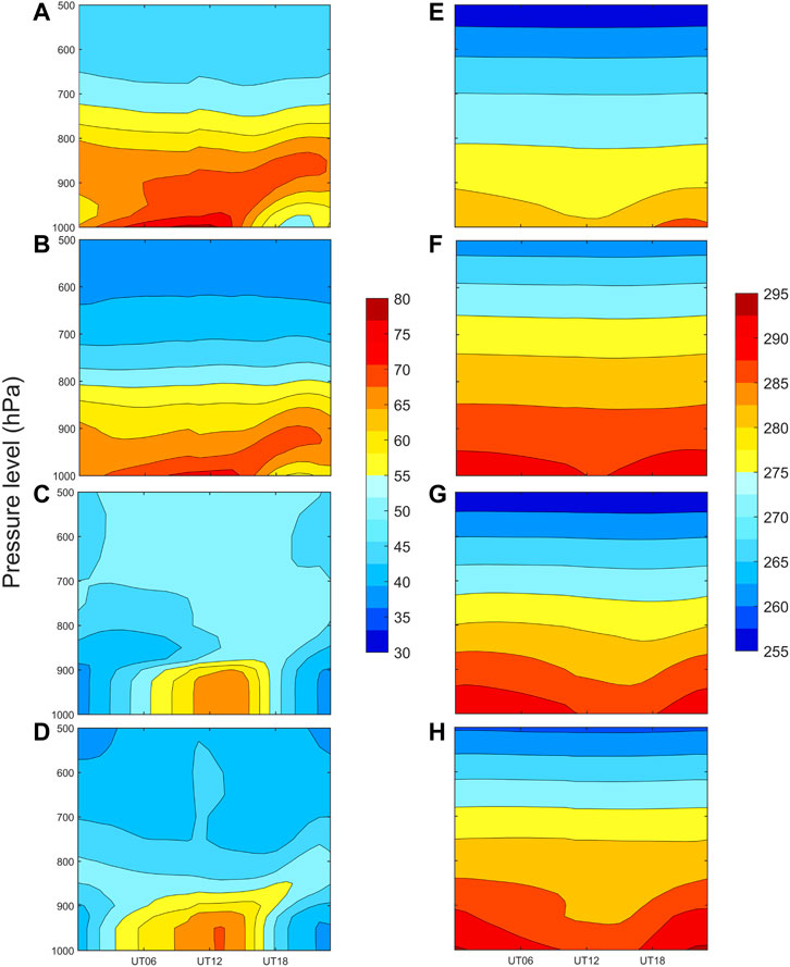
FIGURE 4. Variation of relative humidity (A–D) (unit: %) and temperature (E–H) (unit: K) with altitude and hours in a day. The distribution of figures is the same as that in Figure 3.

As is shown in Figure 3, the seasonal variation of RH varies a lot over the stations, and the variation of the temperature is similar. From Figure 3A, in JJA (June, July, and August) and SON (September, October, and November), a RH low center appears at 500–600 hPa pressure level, while a RH high center appears at 800–900 hPa pressure level. Thus, a large vertical moisture gradient occurs over Albany in JJA and SON, and a relatively small gradient occurs in MAM (March, April, and May). The reason for this seasonal variation over Albany is that Albany belongs to a humid continental climate, and the air in the low layer is humid over the whole year and the precipitation distribution is uniform. In addition, the station is at the windward slope of the Appalachian Mountains, and the moist air from the Atlantic can easily reach Albany. From Figure 3B, a strong RH low center appears at 800–900 hPa pressure level in JJA and the overall RH is low. Hence, a tiny vertical gradient is found over Boise in four seasons. This is mainly because Boise belongs to a semiarid steppe climate, and it shows an obvious continental nature. As a result, the overall humidity is small over Boise. As is shown in Figure 3C, in the upper layer, a RH low center exists in DJF (December, January, and February) and MAM. Moreover, in the low layer, a high center appears in JJA since Charleston belongs to subtropical monsoon climate, and in the summertime, the monsoon from the Atlantic Ocean brings much moisture. Figure 3D gives the distribution of RH over Dodge City. A RH high center appears in DJF and JJA at pressure level 900–1,000 hPa and a low center arises at 500–600 hPa pressure level in JJA and SON. Dodge City also belongs to semiarid steppe climate and the humidity over there is also small. As a result, the moisture gradient in JJA and SON are quite large. With regard to the temperature distribution, as is shown in Figures 3E–H, a warm center appears in summer in the low layer and the cold center appears in the upper layer in DJF and MAM. This can be attributed to the strong solar radiation in summer.

Figure 4 gives a review of the diurnal variation in RH [(a) (b) (c) (d)] and temperature [(e) (f) (g) (h)] over the four stations. For Albany, the RH is high, namely, about 80% in the low layer in UT06-12, and low, that is, approximately 50% in the local daytime. Second, the RH in the upper layer is low in the whole day. As for Boise, the high RH appears at a similar time at the low altitude and the RH is lower in the upper layer. From Figures 4C,D, the high RH center, that is, about 65%, is from UT06-18, and the minimum value of 35% is in the lower layer over Charleston and Dodge City. In the upper layer of the atmosphere, the RH distribution is uniform and the RH over Charleston reaches 50% and the RH over Dodge City reaches lower, that is, approximately 40%. Generally, the moisture gradient over Albany and Boise is bigger than that over Charleston and Dodge City during 1 day. The temperature distribution in a day is similar over the four stations.

Seasonal Variations of Characteristics of Atmospheric Ducts

Duct Frequency

The duct frequency of the four stations in four seasons is presented in Figure 5. The duct frequency is defined as the time of existing ducts divided by twice the size of the number of total days. The ducts are more easily formed in June, July, and August (JJA) and September, October, and November (SON) after taking the overall trend of the four stations into consideration. Among these stations, the occurrence of the atmospheric ducts is the highest in Charleston and the lowest in Boise over the whole year. This phenomenon may result from the differences in the moisture of the two stations based on Figures 3B,C. The RH over Charleston is always high in the lower layer and reaches about 0.75 in JJA for it belongs to subtropical humid climate and much humidity is brought here by the summer monsoon. However, the RH over Boise is continuously low, especially in JJA at the pressure level of 800–900 hPa. This is mainly because Boise belongs to semiarid climate and the moist flow from the Pacific is blocked by the Cordillera Mountains. Thus, the vertical gradient of RH over Charleston is higher than that over Boise.

FIGURE 5

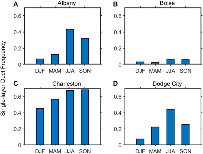
FIGURE 5. Seasonal variation of the single-layer duct frequency over the four stations. (A–D) correspond to Albany, Boise, Charleston, and Dodge City, respectively.

For the Albany station, the highest frequency of ducting appears in JJA with a value of over 0.4 and the lowest appears in DJF with a value of less than 0.1. This station is at the windward slope of the Appalachian Mountains, and the wet and warm flow from the Atlantic Ocean can bring a large amount of moisture to Albany when the monsoon comes in summer. With regard to Dodge City, its climate belongs to semiarid steppe climate. It can also be shown in Figure 3D that the vertical gradient of humidity over the station is relatively greater in JJA and SON. This consists with the ducting occurrence distribution in the four seasons.

The multiple-layer duct frequency over the four stations is presented in Figure 6. The regularity of it consists of all kinds of ducts. The duct frequency is biggest in JJA among four seasons, the overall duct frequency is biggest in Charleston with the value of about 0.35 in JJA, and the lowest frequency is nearly zero over Boise. The reason for this phenomenon may also be related to the vertical moisture gradient.

FIGURE 6

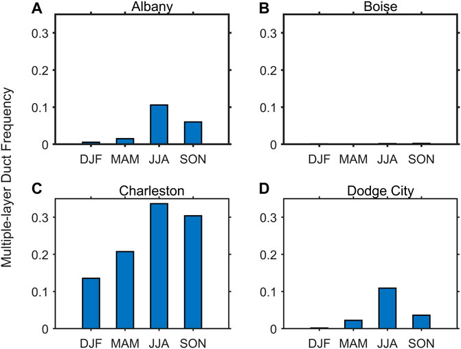
FIGURE 6. The seasonal variation of the multiple-layer duct frequency over the four stations. (A–D) Albany, Boise, Charleston, and Dodge City.

Duct Height

The seasonal variation of the duct height is plotted in Figure 7. The vertical bars represent the standard error. It can be referred that the duct height over Boise is the highest among these four stations and that over Charleston is the lowest over the whole year. Over Boise and Charleston, the general tendencies of each are similar. The maximum average height over Boise appears in SON with the value of about 2,400 m ($\pm 1082$ m) and the minimum average height appears in MAM with a value of about 2,200 m ($\pm 870$ m). For Charleston, the minimum duct height appears in JJA with a value of about 1,400 m ($\pm 1166$ m). Over Albany and Dodge City, the variation trend is similar and the maximum heights are both over 2000 m in JJA. This regularity consists with the law of land ducts that the mean height increases during local summer. This is because at the top of the dry convective boundary layer, ducts are easy to form after solar radiation warms the Earth’s surface. This pattern consists with Figures 3A,B,D, where the RH at the pressure level of 500 hPa in JJA is lower than that in other seasons. This can explain the phenomenon that the duct height over Charleston is the lowest over the whole year. The temperature in the lower layer over Charleston is lower and the height of the boundary layer is lower. Thus, the duct height is lower.

FIGURE 7

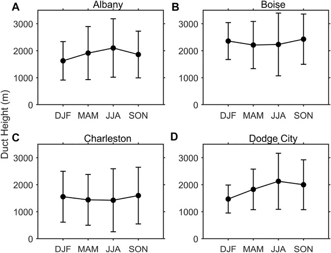
FIGURE 7. Seasonal variation of the duct height over the four stations. (A–D) Albany, Boise, Charleston and Dodge City. The vertical bars are the standard errors.

Duct Strength

The duct strength is the crucial factor for electromagnetic wave propagation. The mean duct strength of the four seasons over four stations is shown in Figure 8. Comparing the four figures with each other, it is found that the duct strength over Charleston reaches the maximum and the strength over Boise is the minimum among the four stations generally. First, over Albany, the strength is lower in DJF and MAM [5 M ($\pm 3$ M)] than in JJA and SON [7 M ($\pm 6$ M)]. For Boise, the seasonal variation of the strength is not obvious. The mean strength is about 5 M throughout the year. For Charleston and Dodge City, the maximum strength over the year appears in MAM and the value is 11 M ($\pm 9$ M) and 9 M ($\pm 9$ M), respectively. To explain the mechanism of the variation, the moisture inversion and temperature inversion are taken into consideration on account of Eq. 1. First, from the aspect of the vertical moisture gradient, over Albany, Charleston, and Dodge City, the vertical gradient is bigger than that of Boise. Second, from the view of the temperature inversion, the vertical temperature gradient is big over the four stations. As a result, it can be concluded that the humidity is the dominant factor in the duct strength. Although Boise and Dodge City are away from the ocean, the moisture from the Pacific Ocean is harder to reach Boise than that from the Atlantic Ocean reaching Dodge City for the difference between the terrain.

FIGURE 8

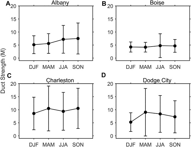
FIGURE 8. Seasonal variation of the duct strength over the four stations. (A–D) Albany, Boise, Charleston and Dodge City. The vertical bars are the standard errors.

Thickness of the Trapping Layer

The impact of the duct on the electromagnetic wave propagation depends on the thickness of the trapping layer. From Figure 9, the seasonal variation of the duct thickness over four stations is presented. Among the four stations, Charleston shows the biggest thickness, that is, over 80 m, and Boise shows the smallest, that is, over 50 m. For Boise, Charleston, and Dodge City, in MAM, the value of the thickness of the trapping layer is, respectively, 60 m ($\pm 20$ m), 80 m ($\pm 40$ m), and 80 m ($\pm 40$ m), which is the greatest in four seasons. However, for Albany, the greatest value occurs in SON with the value of about 70 m ($\pm 30$ m).

FIGURE 9

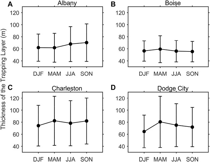
FIGURE 9. Seasonal variation of the thickness of the trapping layer over the four stations. (A–D) Albany, Boise, Charleston and Dodge City. The vertical bars are the standard errors.

Combining with Figures 7–9, it seems that the variation of the duct strength correlates positively with that of the thickness of the trapping layer. In addition, the two parameters seem to show negative correlations with the duct height. This may be because the warmth of the surface can result in the low vertical moisture gradient. However, this can promote dry convection which makes the top of the boundary layer higher. Furthermore, this makes the duct height higher. Figure 10 shows the characteristics of the duct occurring over the four stations. After performing the Pearson correlation analysis between the three characteristics, it is found that the correlation between the strength and thickness is 0.41, which is relatively high. This can also be proved in Figure 8 where the seasonal variations of the two parameters are similar. Furthermore, the duct height correlations with the duct strength and the thickness of the trapping layer are negative, that is, -0.13 and -0.11, which also consists with the conclusion deduced from the seasonal variation of them.

FIGURE 10

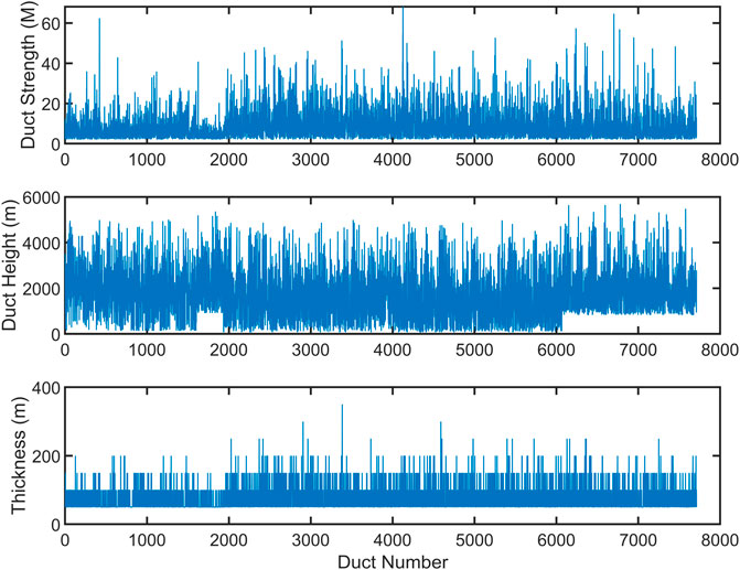
FIGURE 10. Characteristics of ducts, respectively, duct strength, duct height, and the thickness of the trapping layer occurring over the four stations during the observation time.

The Relationship Between the Characteristics of the Ducts and Precipitation

The relationship of weather condition with the occurrence of ducts is investigated in this section. The precipitation data are from the ERA-5 dataset. The seasonal total precipitation of the four stations is as shown in Figure 11. In all, the total precipitation in Albany and Charleston is the highest over the four stations, and that in Boise is the lowest. From the aspect of the climate, this is because Boise belongs to temperate continental climate with low moisture in the atmosphere. Albany and Charleston are located by the sea, and the wet flow from the Atlantic brings the two stations much moisture and then more precipitation over them. With regard to the precipitation relationship with the probability of duct, it is revealed that the precipitation may be correlated with the duct probability positively over Albany, Charleston, and Dodge City, and the relationship may be negative over Boise. This is because over the first three stations, the vertical moisture gradient is the main factor contributing to the duct formation. However, for Boise, the temperature inversion caused by radiative cooling is the main factor. On the other hand, the vertical moisture gradient plays an important role in the rainfall.

FIGURE 11

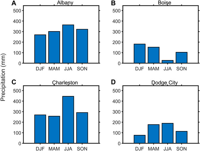
FIGURE 11. Seasonal variation of the total precipitation over the four stations. (A–D) Albany, Boise, Charleston and Dodge City.

Diurnal Variations of Characteristics of Atmospheric Ducts

The parameters of the ducts at UT00 and UT12 are presented in Figure 12. Since the American mainland belongs to the Western 4^th–7^th area, the local time (LT) nighttime and morning time correspond to UT00 and UT12, respectively. First, the diurnal variation of the duct frequency is shown in Figure 12A. For all the stations, the frequency is bigger at UT00 than at UT12. This means that the ducts are formed easily at night than at morning. This is because radiative cooling (Von Engeln et al.) makes the air near the surface cooler than the upper air. Consequently, the temperature inversion appears and the trapping layer starts to form.

FIGURE 12

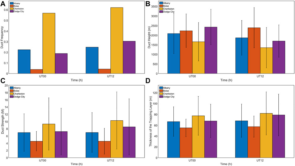
FIGURE 12. Diurnal variation of the duct frequency, the duct height, the duct strength, and the thickness of the trapping layer over the four stations (A–D). The first group of bars of each subgraph represents the parameters at UT00 and the second represents the parameters at UT12.

Figure 12B presents the daily cycle of the ducting height over the four stations. It is found that the duct height at UT00 is generally higher than that at UT12. Dodge City shows the highest height and Charleston shows the lowest height at UT00. At UT12, Charleston still shows the lowest height, while Boise has the highest ducting altitude. The reason for this phenomenon is that the land surface is warmed by solar radiation in the daytime, especially in summer, which makes the dry convection. This leads to the growth of the boundary layer, and then the duct height is higher in the daytime than in the nighttime.

Second, from Figure 12C, combining the strengths of the four stations with each other, it is revealed that the strength at UT00 is commonly smaller than that at UT12. Charleston shows the biggest strength and Boise shows the smallest strength both in the day and night. This is mainly because UT00 corresponds to the daytime in America and UT12 corresponds to the nighttime. It is revealed that land events have more strength during the nighttime due to the temperature inversions generated by radiative cooling.

As for the diurnal variation of the thickness of the trapping layer, it is vividly shown in Figure 12D. The thickness shows similar regularity with the duct height. At UT00, Charleston shows the biggest thickness and Boise shows the smallest thickness. The situation is the same at UT12.

Conclusion

In this work, GPS radiosonde data from RRS, SRTM15 Elevation data, and ERA-5 reanalysis data are combined to investigate different characteristics of the ducts over the four stations. This work is important for the radio communication since this structure can not only make the propagation path longer but also make up the blind zones.

The research can be divided into two parts: one is the seasonal variation over the four stations and the other is the diurnal variation over the stations. First, from the seasonal aspect, the duct frequency over Charleston is the biggest and the frequency over Boise is the smallest among the four stations generally in the whole year. This results from the differences between the vertical moisture over the stations and between different seasons. In addition, the duct frequency is higher in JJA and SON. Generally speaking, the probability of duct increases with the increase in the vertical moisture gradient. The duct height is the highest over Boise and the lowest over Charleston, and the height tends to increase in JJA and SON for the solar radiation makes the dry air near the surface rise and then makes the top of the dry boundary layer easier to form atmospheric ducts.

The distribution of the duct strength is similar to that of the duct frequency. The overall duct strength over Charleston is the biggest, and the strength over Boise is the smallest. This phenomenon can also be explained with the vertical moisture gradient. Finally, the variation in the thickness of the trapping layer is presented. It is revealed that the thickness is also the biggest over Charleston and the smallest over Boise. In summary, the seasonal variation of the duct frequency, duct strength, and the thickness of the trapping layer is almost the same. Moreover, the duct height shows the inverse tendency. In addition, the total precipitation is related with the duct probability positively over the coastal areas and the relation is negative over the desert and tropical areas.

From the diurnal variation aspect, with regard to the duct frequency, it is bigger at UT00 than at UT12 for radiative cooling. For the duct height, the height at daytime is always higher than that at nighttime since the dry convection from the bottom leads to the growth of the boundary layer. Next, the duct strength tends to be bigger at nighttime than at daytime. This results from the temperature inversion caused by radiative cooling. Finally, the diurnal variation of the thickness of the trapping layer is similar basically over four stations. The probability of a multiple-layer duct is investigated, too. It is found that the law of its seasonal variation consists with the variation of the duct strength and probability.

In all, this work investigates the characteristics of the duct over different parts of America, and the differences between the characteristics are explained. Based on these explanations and conclusions, the regularity of the duct is revealed, and this work can be helpful for EMW propagation over the land. Furthermore, this work can be of value to the research of the characteristics of the ducts in other areas of the world.

Data Availability Statement

Publicly available datasets were analyzed in this study. These data can be found here: https://cds.climate.copernicus.eu/cdsapp#!/home https://www.sparc-climate.org/data-centre/data-access/us-radiosonde/ http://www.tuxingis.com.

Author Contributions

Conceptualization, XZ; methodology, LH; software, LH and YL; validation, LH; formal analysis, LH; investigation, XZ and LH; resources, LH; data curation, LH; writing—original draft preparation, LH; writing—review and editing, LH, XZ, and YL; supervision, XZ; project administration, XZ and YL; funding acquisition, XZ.

Funding

This work was supported by the National Natural Science Foundation of China (Grant No. 41775027).

Conflict of Interest

The authors declare that the research was conducted in the absence of any commercial or financial relationships that could be construed as a potential conflict of interest.

Publisher’s Note

All claims expressed in this article are solely those of the authors and do not necessarily represent those of their affiliated organizations, or those of the publisher, the editors, and the reviewers. Any product that may be evaluated in this article, or claim that may be made by its manufacturer, is not guaranteed or endorsed by the publisher.

References

Babin, S. M., and Rowland, J. R. (1992). Observation of a Strong Surface Radar Duct Using Helicopter Acquired Fine-Scale Radio Refractivity Measurements. Geophys. Res. Lett. 19, 917–920. doi:10.1029/92GL00562

CrossRef Full Text | Google Scholar

Bolton, D. (1980). The Computation of Equivalent Potential Temperature. Mon. Wea. Rev. 108 (7), 1046–1053. doi:10.1175/1520-0493(1980)108<1046:tcoept>2.0.co;2

CrossRef Full Text | Google Scholar

Ding, J., Fei, J., Huang, X., Cheng, X., and Hu, X. (2013). Observational Occurrence of Tropical Cyclone Ducts from GPS Dropsonde Data. J. Appl. Meteorology Climatol. 52 (5), 1221–1236. doi:10.1175/JAMC-D-11-0256.1

CrossRef Full Text | Google Scholar

Haack, T., and Burk, S. D. (2001). Summertime Marine Refractivity Conditions along Coastal California. J. Appl. Meteor. 40 (4), 673–687. doi:10.1175/1520-0450(2001)040<0673:smrcac>2.0.co;2

CrossRef Full Text | Google Scholar

Han, J., Wu, J.-J., Zhu, Q.-L., Wang, H.-G., Zhou, Y.-F., Jiang, M.-B., et al. (2021). Evaporation Duct Height Nowcasting in China's Yellow Sea Based on Deep Learning. Remote Sens. 13 (8), 1577. doi:10.3390/rs13081577

CrossRef Full Text | Google Scholar

Karimian, A., Yardim, C., Gerstoft, P., Hodgkiss, W. S., and Barrios, A. E. (2011). Refractivity Estimation from Sea Clutter: An Invited Review. Radio Sci. 46 (6). doi:10.1029/2011RS004818

CrossRef Full Text | Google Scholar

Kursinski, E., Hajj, G., Leroy, S., and Herman, B. (2000). The GPS Radio Occultation Technique. Terr. Atmos. Ocean. Sci. 11 (1), 53–114. doi:10.3319/tao.2000.11.1.53(cosmic)

CrossRef Full Text | Google Scholar

Li, X., Sheng, L., and Wang, W. (2021). Elevated Ducts and Low Clouds over the Central Western Pacific Ocean in Winter Based on GPS Soundings and Satellite Observation. J. Ocean. Univ. China 20 (2), 244–256. doi:10.1007/s11802-021-4510-0

CrossRef Full Text | Google Scholar

Mai, Y., Sheng, Z., Shi, H., Liao, Q., and Zhang, W. (2020). Spatiotemporal Distribution of Atmospheric Ducts in Alaska and its Relationship with the Arctic Vortex. Int. J. Antennas Propag. 2020, 1–13. doi:10.1155/2020/9673289

CrossRef Full Text | Google Scholar

Manjula, G., Roja Raman, M., Venkat Ratnam, M., Chandrasekhar, A. V., and Vijaya Bhaskara Rao, S. (2016). Diurnal Variation of Ducts Observed over a Tropical Station, Gadanki, Using High-Resolution GPS Radiosonde Observations. Radio Sci. 51 (4), 247–258. doi:10.1002/2015RS005814

CrossRef Full Text | Google Scholar

Rogers, L. T., Hattan, C. P., and Stapleton, J. K. (2000). Estimating Evaporation Duct Heights from Radar Sea Echo. Radio Sci. 35 (4), 955–966. doi:10.1029/1999RS002275

CrossRef Full Text | Google Scholar

Sirkova, I. (2015). Duct Occurrence and Characteristics for Bulgarian Black Sea Shore Derived from ECMWF Data. J. Atmos. Solar-Terrestrial Phys. 135, 107–117. doi:10.1016/j.jastp.2015.10.017

CrossRef Full Text | Google Scholar

Smith, E., and Weintraub, S. (1953). The Constants in the Equation for Atmospheric Refractive Index at Radio Frequencies. Proc. IRE 41, 1035–1037. doi:10.1109/jrproc.1953.274297

CrossRef Full Text | Google Scholar

Sun, Z., Ning, H., Song, S., and Yan, D. (2016). First Observations of Elevated Ducts Associated with Intermittent Turbulence in the Stable Boundary Layer over Bosten Lake, China. JGR Atmos. 121 (19), 201–214. doi:10.1002/2016JD024793

CrossRef Full Text | Google Scholar

Von Engeln, A. (2004). A Ducting Climatology Derived from the European Centre for Medium-Range Weather Forecasts Global Analysis Fields. J. Geophys. Res. 109 (D18), D18104. doi:10.1029/2003JD004380

CrossRef Full Text | Google Scholar

Yan, X., Yang, K., and Ma, Y. (2018). Calculation Method for Evaporation Duct Profiles Based on Artificial Neural Network. Antennas Wirel. Propag. Lett. 17 (12), 2274–2278. doi:10.1109/LAWP.2018.2873110

CrossRef Full Text | Google Scholar

Yardim, C., Gerstoft, P., and Hodgkiss, W. S. (2008). Tracking Refractivity from Clutter Using Kalman and Particle Filters. IEEE Trans. Antennas Propagat. 56 (4), 1058–1070. doi:10.1109/TAP.2008.919205

CrossRef Full Text | Google Scholar

Zhao, W., Zhao, J., Li, J., Zhao, D., Huang, L., Zhu, J., et al. (2021). An Evaporation Duct Height Prediction Model Based on a Long Short-Term Memory Neural Network. IEEE Trans. Antennas Propagat. 69, 7795–7804. –1. doi:10.1109/TAP.2021.3076478

CrossRef Full Text | Google Scholar

Zhu, X., Li, J., Zhu, M., Jiang, Z., and Li, Y. (2018). An Evaporation Duct Height Prediction Method Based on Deep Learning. IEEE Geosci. Remote Sens. Lett. 15 (9), 1307–1311. doi:10.1109/LGRS.2018.2842235

CrossRef Full Text | Google Scholar