Research and Application of the Mode Decomposition-Recombination Technique Based on Sample-Fuzzy Entropy and K-Means for Air Pollution Forecasting

Practical forecasting of air pollution components is important for monitoring and providing early warning. The accurate prediction of pollutant concentrations remains a challenging issue owing to the inherent complexity and volatility of pollutant series. In this study, a novel hybrid forecasting method for hourly pollutant concentration prediction that comprises a mode decomposition-recombination technique and a deep learning approach was designed. First, a Hampel filter was used to remove outliers from the original data. Subsequently, complete ensemble empirical mode decomposition adaptive noise (CEEMDAN) is employed to divide the original pollution data into a finite set of intrinsic mode function (IMF) components. Further, a feature extraction method based on sample-fuzzy entropy and K-means is proposed to reconstruct the main features of IMFs. In conclusion, a deterministic forecasting model based on long short-term memory (LSTM) was established for pollutant prediction. The empirical results of six-hourly pollutant concentrations from Baoding illustrate that the proposed decomposition-recombination technique can effectively handle nonlinear and highly volatile pollution data. The developed hybrid model is significantly better than other comparative models, which is promising for early air quality warning systems.

Introduction

Following rapid industrialization and urbanization, various air pollution problems have occurred frequently. Air pollution has serious effects on human health and causes significant economic losses (Tang et al., 2010; Liu et al., 2011; Pandey et al., 2021). Therefore, establishing high-precision monitoring and prediction models is necessary to support governmental decision-making, environmental protection, and medical diagnosis.

Up to now, enormous amount of studies contributed to predicting future trends of air pollutants. In summary, most works modeled for prediction from three perspectives: mathematical and physical techniques, statistical prediction models, and machine learning models. First, mathematical and physical techniques have long been widely used in the field of air pollutant prediction. For instance, Huang et al. (2018) developed a random forest model, including gap-filled aerosol optical depth (AOD), Modern-Era Retrospective analysis for Research and Applications Version 2 (MERRA-2) simulations, meteorological parameters, and land cover as predictors to estimate monthly PM_2.5 concentrations in North China. Tessum et al. (2015) used Weather Research and Forecasting with Chemistry Meteorological (WRF-Chem) and a chemical transport model (CTM) to simulate air pollution in adjacent areas of the United States for 12 months in 2005 with a horizontal resolution of 12 km and evaluated the simulation results. Atmospheric environment diffusion model techniques such as CTM and WRF can predict the pollutant concentration by solving the corresponding differential equation, which makes the prediction more deterministic (Yahya et al., 2014). Pollutants can further be predicted using the statistical forecasting model. Statistical methods are used to predict pollutants by mining time-series data for characteristic information. Zhang et al. (2018) used the autoregressive integrated moving average model (ARIMA) to predict the PM_2.5 concentration and compared it with other pollutant concentrations and meteorological parameters. Further, Wang P. et al. (2017) proposed a novel hybrid generalized autoregressive conditional heteroskedasticity (GARCH) method by combining ARIMA and support vector machine (SVM) forecasting models. Additionally, some improved statistical models, such as multiple linear regression (Elbayoumi et al., 2015; Yuchi et al., 2019; Yan and Enhua, 2020) and gray models (Chen & Pai, 2015; Wu & Zhao, 2019), are proposed for better prediction of PM2.5. Machine learning models such as artificial neural networks and support vector algorithms have recently become more prominent in pollution prediction. Various machine learning methods have been used in previous air pollution prediction studies. These include the following: backpropagation neural network (BPNN) (Bai et al., 2016); generalized regression neural network (GRNN) (Zhou et al., 2014); extreme learning machine (ELM) (Shang et al., 2019); random forest (Huang et al., 2018); support vector regression (SVR) (Zhu et al., 2018); long short-term memory (LSTM) (Qi et al., 2019; Yan et al., 2021) Zhang et al. (Zhang et al., 2019), integrated a multiple objectives model with five algorithms—BPNN, ARIMA, cuckoo search (CS), holt winters (HW) and online extreme learning machine (OELM)—for wind speed prediction. A constructed function comprising a three-objective combined model was optimized using a non-dominated sorting genetic algorithm. Liu et al. (Liu et al., 2018), constructed a combined model was constructed using a nonlinear neural network and statistical linear algorithm. Compared with several integrated models, it is more reliable and results in high accuracy.

However, it is hardly possible for a single prediction method to elaborately capture all complex features in pollution series which locate in a high dimension space. To this end, data preprocessing by outlier removing and series decomposition is efficient way for model construction at first. Various data preprocessing methods are developed for pollution data with nonlinearity and volatility present in. Data preprocessing approaches and optimization strategies have been extensively researched for pollutant prediction to increase the efficiency and accuracy of the prediction performance (Li & Zhu, 2018). Researchers usually propose suitable data preprocessing methods and process them according to study requirements. Several existing data preprocessing methods are relevant to the study of environmental contaminants. Empirical Mode Decomposition (EMD) (Huang et al., 1998) is a well-known algorithm for series decomposition. This algorithm projects a time series onto a set of intrinsic mode function (IMF) acting as bases because the project coefficients show good shapes via the Hilbert transform. These bases are derived from the phenomena of oscillations in the physical time domain. Owing to the poor performance of the subjective intervention for the intermittence test, EEMD (Wu and Huang, 2009) is proposed using noise-assisted data analysis (NADA) to construct a set of IMF. To increase the scales of a series at high frequency via the transformation of the IMF, an ensemble of white noise is incorporated for the designed trials because its scales are distributed uniformly in both the time and frequency domains. The true signal is estimated using the average of the ensemble in which the random white noise is canceled out, and only the persistent part of the signal remains. For example, (Zhou et al., 2014), suggested a hybrid ensemble empirical mode decomposition-generalized regression neural network (EEMD-GRNN) model that integrates the EEMD and a generalized regression neural network (GRNN) as a strategy for forecasting PM_2.5. Wang (Wang D. et al., 2017) developed a new hybrid model based on a two-phase decomposition technique and modified ELM to improve the forecasting accuracy of the air quality index. Xu et al. (Xu et al., 2017) developed a hybrid model based on Improved Complementary Ensemble Empirical Mode Decomposition, Whale Optimization Algorithm and Support Vector Machine (ICEEMD-WOA-SVM) to predict major pollutants, in which the data preprocessing part follows a “decomposition and integration” strategy. The raw series of each pollutant concentration was decomposed into several IMFs that were individually decomposed using a data preprocessing technique. The Hampel filter is an offline frequency-domain filtering method for eliminating spectral outliers (Allen, 2009). The advantage of the Hampel filter is that there is no prior need to know the outliers where the disturbance occurs. Moreover, the processed data series will not be distorted. Li et al. (Li et al., 2019) developed a new analysis and prediction system for air quality index prediction. Outliers in the air quality index series were eliminated using Hampel filter. Liu et al. (Liu and Chen, 2020) proposed a three-stage hybrid neural network model for outdoor PM_2.5 forecasting. K-means is an iterative clustering analysis algorithm used in pollutant data analysis. Riches et al. (Riches et al., 2022) employed the K-means cluster to analyze five concentrations. They further examined the patterns of association between PM_2.5, PM_10, CO, NO₂, O₃, and SO₂ measurements and variations in annual diabetes incidence at the county level in the United States.

The data preprocessing methods mentioned above provided qualified data for later analysis with prediction models. However, most current studies only use a single data preprocessing technology which cannot offer well present data suitable for further modeling. For example, in some studies, the EEMD technique was the only method used to decompose the original data into numerous IMF components for reducing the prediction complexity. The effective extraction of features from IMFs is difficult because features with diversity in frequency domain might be caused by outliers, which introduce disturbance into prediction. Therefore, in this study, the original data were first filtered by Hampel to eliminate the outliers in the data. The data were then decomposed into several IMFs using complete ensemble empirical mode decomposition adaptive noise (CEEMDAN). The complexity characteristics of the different sequences were obtained by calculating the fuzzy entropy and information entropy of each IMF signal. Subsequently, similar IMFs are recombined using the K-means clustering method based on fuzzy entropy and information entropy. After that, a prediction model was established using LSTM to conduct an empirical study of the six pollutants.

Related Methodologies

Data Preprocessing Method

Six data preprocessing methods—the Hampel filter, CEEMDAN, Sample entropy (SE), Fuzzy entropy (FE), K-means, and LSTM prediction methods—were applied in this study to better predict the concentrations of six pollutants: PM_2.5, PM₁₀, SO₂, NO₂, O₃, and CO. First, the original data were filtered by Hampel filter to eliminate the outliers in the data. Then, the data was decomposed into several IMFs using CEEMDAN. The complicated characteristics of the different sequences were obtained by calculating the fuzzy entropy and information entropy of each IMF signal. Finally, to sum up similar IMFs in each group clustered with the K-means in terms of fuzzy entropy and information entropy.

Hampel Filter

The Hampel filter is an offline frequency-domain filtering method used to eliminate spectral outliers that are difficult to represent elaborately using prediction models. By representing the sequence with a one-dimensional vector, the method generates a local window around each element of the vector and calculates the median of all elements in that window. The standard deviation of each sample was further estimated using the absolute value of the median. The absolute difference between the sample and median shorted in the MAD can be a direct measurement for outlier detection. Mathematically, the Hampel filter detects elements as outliers in a vector using Eq. 1:

$\{\begin{array}{c}{S}_j=1.4286median\left\{\left|x_j-x_j^{\ast }\right|\right\},\\ x_j=x_j^{\ast },\text{if}\left|x_j-x_j^{\ast }\right|>t{S}_j,\text{for}j=1,\mathrm{...},N,\end{array}(1)$

where $t$ is the threshold, and $N$ is the length of the vector. The variables $x_j^{\ast }$ and $S_j$ are the median and standard deviation of the window centered at element $x_j$, respectively. The deviation $S_j$ is estimated adaptively by multiplying MAD and a constant. Element $x_j$ is further replaced with $x_j^{\ast }$ when the MAD is $t$ times larger than $S_j$, the standard deviation.

Algorithm of CEEMDAN

EEMD can obtain better IMF than EMD. However, it does not result in exact decomposition because the white noise drives the generation on new modes that hide within the mixed IMFs. Furthermore, the IMF might not be orthogonal so that the energy of the added white noise is not similar to that when the polluted series are expanded by the IMF. To overcome this problem, CEEMDAN first defines a residual between the series and variation IMF from EEMD and then applies the step in EMD, which extracts the most IMF of the residual. The above steps were repeated until the residual energy was small. The last residual is defined as the last mode, which is why this algorithm is considered complete.

Let $E_1(•)$ denote the operator that decomposes the first mode from a series, defined as in EMD, and let $IM{F}_j^{\text{V}}$ denote the variation of the $j-\text{th}$ IMF. Assuming $M$, the number of trials in EEMD, the procedure of CEEMDAN is described in detail as follows:

Step 1: The first variation IMF is the same as the first in EEMD.

$IM{F}_1^{\text{v}}\left[n\right]=\frac{1}{M}{\displaystyle \sum _{i=1}^{M}IM{F}_1^i\left[n\right]}=\overline{IM{F}_1}\left[n\right].$

Step 2: The following is the first residual off the decomposed series.

$r_1\left[n\right]=x\left[n\right]-IM{F}_1^{\text{v}}\left[n\right].$

Step 3: Let the second mode be the mean of the decompositions of the residuals enhanced by adaptive noise with $E_1(•)$ in an ensemble of trials.

$IM{F}_2^{\text{v}}\left[n\right]=\frac{1}{M}{\displaystyle \sum _{i=1}^M{E}_1\left(r_1\left[n\right]+{\epsilon }_1{E}_1\left({\omega }^i\left[n\right]\right)\right)}.$

Step 4: Similar to step 2, define the $k-\text{th}$ residual off the $\left(k-1\right)-\text{th}$ residual.

$r_k\left[n\right]=r_{\left(k-1\right)}\left[n\right]-IM{F}_k^{\text{v}}\left[n\right].$

Step 5: Extract the $\left(k+1\right)-\text{th}$ mode, $IM{F}_{k+1}^{\text{V}}\left[n\right]$, from the enhanced $k-\text{th}$ residual by an adaptive noise,

$IM{F}_{\left(k+1\right)}^{\text{v}}\left[n\right]=\frac{1}{M}{\displaystyle \sum _{i=1}^M{E}_1\left(r_k\left[n\right]+{\epsilon }_k{E}_k\left({\omega }^i\left[n\right]\right)\right)}.$

Step 6: After the number of $K$ decompositions, the last residual is given as follows:

$R\left[n\right]=x\left[n\right]-{\displaystyle \sum _{k=1}^{K}IM{F}_k^{\text{v}}},$

and we have the exact decomposition

$x\left[n\right]={\displaystyle \sum _{k=1}^{K}IM{F}_k^{\text{v}}+R\left[n\right]}.$

Sample Entropy

Sample entropy is a new measure of time-series complexity proposed by Richman and Moornan (Richman et al., 2000), which aims to reduce the error of the approximate entropy algorithm with higher accuracy. Sample entropy was calculated as follows:

From a time series $X=\left[x_{1,}{x}_{2,}\cdots ,x_n\right],$ and a tolerance $r$,

Step 1:Generate a group of vector by rolling on time,

$X_i^m=\left[x_i,x_{i+1},\cdots ,x_{i+m-1}\right],i=\mathrm{1,2},\mathrm{...},n-m+1.$

Step 2: Define the distance between $X_i^m$ and $X_j^m$ with the maximum norm of $X_i^m-X_j^m$,

$d_{ij}^m=d\left( X_i^m ,X_j^m \right)=\max \left\{\left|x_{i+k}-x_{j+k}\right|,k=\mathrm{0,1},\cdots ,m-1\right\}.$

Step 3:For each $i,i=1,\dots ,n-m+1$, calculate $P_i^m\left(r\right)$ by the sum of indicate function $I(•)$, $P_i^m\left(r\right)=\frac{1}{n-m}{\displaystyle \sum _{j\ne i}I\left(d_{ij}^m<r\right)}$, and ${\varphi }^m\left(r\right)=\frac{1}{n-m+1}{\displaystyle \sum _{i=1}^{n-m+1}{P}_i^m\left(r\right)}$.

Step 4:Let $m=m+1$, and repeat steps 1–3, get ${\varphi }^{m+1}\left(r\right)$, then the sample entropy is defined as

$S{E}^m\left(r\right)=-\ln \left(\frac{{\varphi }^{m+1}\left(r\right)}{{\varphi }^m\left(r\right)}\right)(2)$

Fuzzy Entropy

The concept of fuzzy sets was first introduced by Zadeh (Zadeh, 1965), which resulted in the formation of fuzzy entropy with further research on fuzzy sets. The statistical measure of fuzzy entropy was further developed by Chen et al. (Chen et al., 2009) to characterize the degree of fuzziness of fuzzy sets. As a measure of complexity, there is less bias, and continuity is achieved as well as free parameter selection and greater robustness against noise.

There are many definitions of fuzzy entropy as long as the definition satisfies the four rules described in this study (Zadeh, 1965). In this study, fuzzy entropy is similarly formulated as part of the sample entropy. The first difference is that a constant $c$ is subtracted from all the elements of the vector $X_i^m$ generated by rolling on time:

$X_i^m=\left[x_i,x_{i+1},\cdots ,x_{i+m-1}\right]-c,i=\mathrm{1,2},\mathrm{...},n-m+1,$

where $c=\frac{1}{m}{\displaystyle {\sum }_{k=i}^{i+m-1}k.}$ The second difference is the definition of distance for two vectors,

$d_{ij}^m=\exp \left\{-{\left(\frac{{\left|X_i^m-X_j^m\right|}_{\max }}{r}\right)}^2\right\}.$

The other steps are similar to those of the sample entropy. In conclusion, the fuzzy entropy is defined as

$FuzzyEn\left(t\right)=\ln {\varphi }^m\left(t\right)-\ln {\varphi }^{m+1}\left(t\right).(3)$

K-Means

The K-means algorithm is a classic method for clustering points in high-dimensional space, as proposed by Macqueen (Macqueen, 1967). Based on the criterion of similarity between two points, usually measured by the Euclidean distance, a point is determined to belong to the class whose center is closest to it. The centers of all groups are updated after all points in the dataset are set. The algorithm stops when the cluster measurement function converges, which means that there are no changes for all centers in the updating.

The distance and similarity between points $X_i$ and $C_j,$ the center of the jth class, can be calculated as follows:

$d\left(x_i,c_j\right)=\sqrt{{\left(x_i^1-c_j^1\right)}^2+\mathrm{...}+{\left(x_i^k-c_j^k\right)}^2+\mathrm{...}+{\left(x_i^d-c_j^d\right)}^2},$

$s\left(x_i,c_j\right)=1/d\left(x_i,c_j\right).$

For each updated class, a new cluster center is calculated. Assuming that the samples in the jth class are $\left\{x_{j1},x_{j2},\mathrm{...},x_{j{n}_j}\right\}$ and the cluster center is $c_j=\left(c_j^1,c_j^2,\mathrm{...},c_j^k,\mathrm{...},c_j^d\right)$, the kth attribute of class center $C_j$ is represented as $C{K}_j$, which is

$c_j^k=\frac{x_{j1}^k+x_{j2}^k+\mathrm{...}+x_{j{n}_j}^k}{n_j}.$

The above process is repeated until the standard measure function converges. The conventional clustering measure function is usually the mean-square deviation, which is expressed as

$J=\sqrt{\frac{{\displaystyle \sum _{i=1}^k{\displaystyle \sum _{j=1}^{n_j}{\left(x_{ij}-c_i\right)}^2}}}{n-1}}.(4)$

LSTM

LSTM is a type of recurrent neural network (RNN), which was originally established by Hochreiter and Schmidhuber (Aksoy et al., 2018) and was refined and popularized by many others in subsequent work. RNN are sensitive to short-term information. However, they always have a problem of long-term reliance. As an improvement to RNN, LSTM solves this problem by introducing a cell state in which the long-term state is saved. In this neural network, there are some LSTM blocks, which are regarded as intelligent net cells in certain studies. In several versions of LSTM, the most important LSTM cell is “forget gate.” There are four neural network layers, each of which interacts in a unique manner.

The first stage of LSTM is to identify the information from the cell state that should be forgotten or rejected. The “forget gate layer,” formulated by a sigmoid layer, makes this judgment. For input $h_{t-1}$ and $x_t$, a number between zero and one is the output for each number in the cell state $C_{t-1}$. Output 1 means “keep this completely,” while 0 means “forget this completely.” This step is formulated as follows:

$f_t=\sigma \left(W_f\cdot \left[h_{t-1},x_t\right]+b_f\right).(5)$

where $h_{t-1}$ is the output of the previous input value, representing the effect on the current input value. Matrix $w_f$ is the weight of the input value, and $b_f$ is the deviation of the input value. Output $f_t$ is the result of function $\sigma$, a 0–1 output function.

We further determine which part of the information needs to be stored in the cell state. The “input gate layer” $i_t$ first determines which values will be updated. Denoting $\stackrel{\text{∼}}{C_t}$ as the “tanh layer,” a vector is generated for new candidate values. These two layers are further integrated to update the state.

$i_t=\sigma \left(W_{\dot{I}}\cdot \left[h_{t-1},x_t\right]+b_i\right)$

$\stackrel{\text{∼}}{C_t}=\tanh \left(W_C\cdot \left[h_{t-1},x_t\right]+b_C\right)$

where tanh is a function of hyperbolic arctangent. The other parameters are similar to those in Eq. 5.

The next step is to multiply the old state by $f_t$, forgetting the information that should be rejected earlier. This is implemented using the following operation:

$C_t=f_t\ast C_t+i_t\ast {\stackrel{\sim }{C}}_t$

In conclusion, the unit state $O_t$ is determined by the output of the sigmoid layer. Subsequently, the cell state is transformed by the tanh function, which outputs a value between 1 and -1. For the next recurrent, $h_t$ is the multiplication of the unit state and tanh transform of the cell state. This is formulated as

$O_t=\sigma \left(W_o\left[h_{t-1},x_t\right]+b_o\right),$

$h_t=o_t\ast \tanh \left(C_t\right).(6)$

Hybrid Model Architecture

This section introduces the proposed hybrid model architecture, which includes the following three parts: data preprocessing, pollutant concentration prediction, and model evaluation. Figure 1 shows a framework diagram of the proposed model.

FIGURE 1

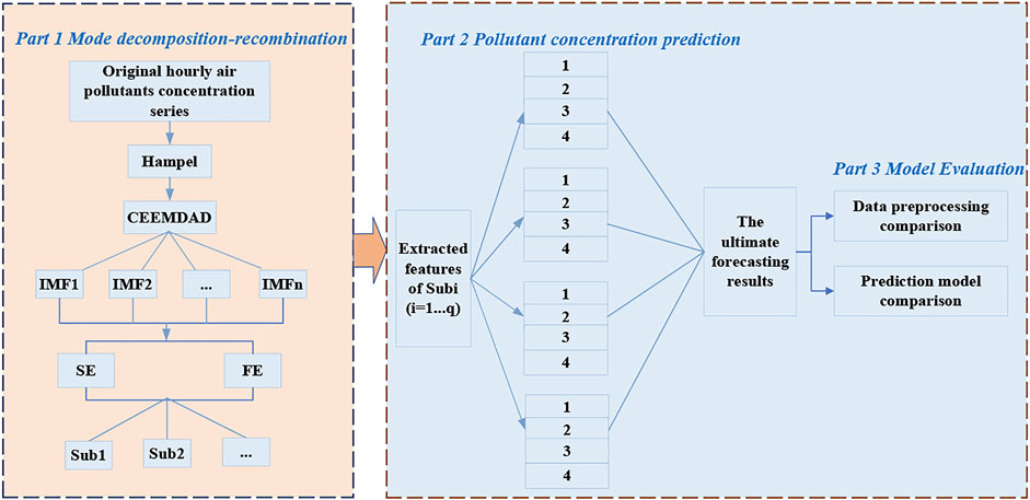
FIGURE 1. The framework diagram of the hybrid model.

Part 1 Mode Decomposition-Recombination

Step 1: Original data were filtered using Hampel filtering to eliminate outliers.

Step 2: The filtered data were decomposed into several IMF component sequences using CEEMDAN.

Step 3: Calculated the information entropy and fuzzy entropy of each IMF component into a two-dimensional vector.

Step 4: Based on the calculation results of the information entropy and fuzzy entropy, K-means was used to cluster the IMF components to achieve feature extraction.

Part 2 Pollutant Concentration Prediction

Step 1: For each data group obtained from clustering, the 4-fold cross-validation method was used for training.

Step 2: Setting up the LSTM model structure, the hidden layer was selected as a 2-layer LSTM structure, the number of neuron nodes in the first layer was 64, the number of neuron nodes in the second layer was 32, and the output layer reduced the results to the original data format.

Step 3: The mean absolute error (MAE) was chosen as the loss function, the Adam algorithm was used to generate optimization parameters for each node learning, and the error was reduced by iterating and adjusting the weights until convergence.

Step 4: To obtain the final prediction results, the prediction results of each group were superimposed.

Part 3 Model Evaluation

Step 1: Designed model evaluation experiments. In this study, we designed two sets of evaluation experiments: 1) data preprocessing comparison; 2) prediction model comparison.

Step 2: In the data preprocessing comparison experiments, we chose three comparison models: 1) the LSTM model without data preprocessing; 2) Hampel integrated with the LSTM model; 3) the CEMMDAN integrated LSTM model with our proposed SFE-K-Means integrated LSTM model for the comparison experiments.

Step 3: For the prediction model comparison experiments, we chose the backpropagation neural network (BPNN), evolutionary neural network (ENN), and Extreme Learning Machine (ELM), which are the three benchmark comparison models for comparison with the LSTM model and our proposed model.

Step 4: We chose mean squared error (RMSE), MAE, and mean absolute percentage error (MAPE) as the model evaluation criteria for the above two sets of experiments.

Empirical Study

Data Description

Major air pollutants in the atmosphere, including PM_2.5, PM₁₀, SO₂, CO, NO₂ and O₃, were selected as the research objects in this study. The Ministry of Environmental Protection of the People’s Republic of China (http://www.mep.gov.cn/) has provided six pollutant concentration datasets from Baoding. Sample data were collected on September 1, 2017, and November 30, 2017, in Baoding. The hourly pollution concentration data totaled 2140. These datasets were split into two categories: training and testing. The first 1814 data (approximately 85% of the total data) are training sets, and 321 data points (approximately 15%) for test.

Performance Evaluation Criteria

This study considers three assessment criteria, as in Table 1, to effectively evaluate the performance of the model. MAE, MSE and MAPE were chosen as error criteria to reflect the prediction performance of the forecasting models.

TABLE 1

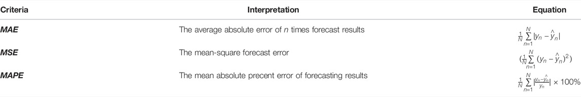
TABLE 1. Evaluation criteria.

Mode Decomposition-Recombination Technique Process

Results of Outlier Detection

The series of original environmental pollution concentrations have obvious volatility and nonlinear characteristics and contain a few outliers. Therefore, data preprocessing is required for the original data. This section first uses a Hampel filter to process the original data. The filtering results of the six pollutant time series are shown in Figure 2, which shows that the filtered time series present more smooth appearance and more stable variation in local area after outliers and noise are eliminated from the original data.

FIGURE 2

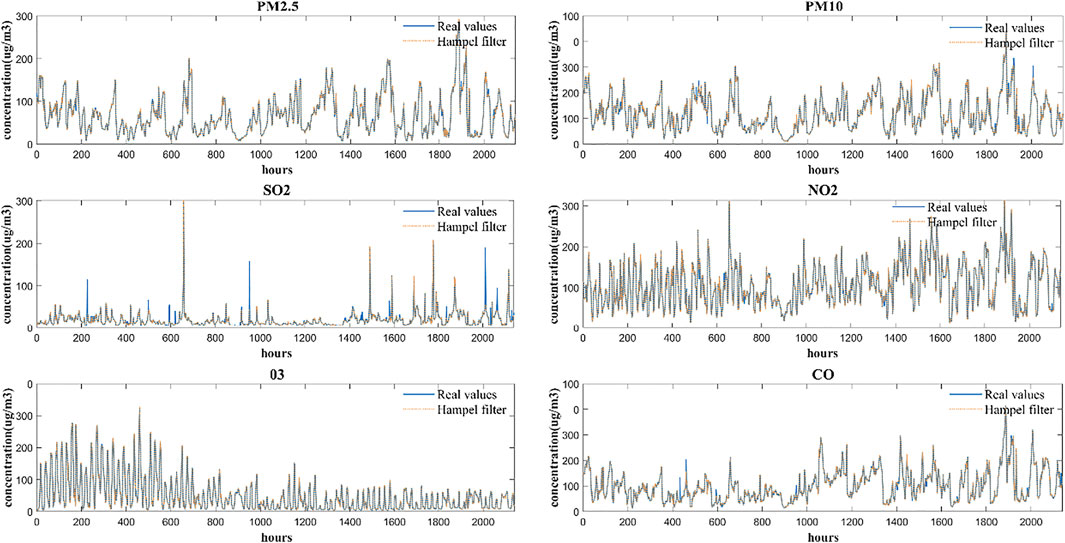
FIGURE 2. Filtering results of the six pollutants time series.

Results of Decomposition for Six Pollutants Data

In this section, CEEMDAN is used to decompose the original amount of pollutant series into a collection of IMFs with associated frequencies and the residue component. We chose an ideal standard deviation of 0.1–0.5 and a total of 200 ensemble members. The original pollutant series decomposed using CEEMDAN is shown in Figure 3.

FIGURE 3

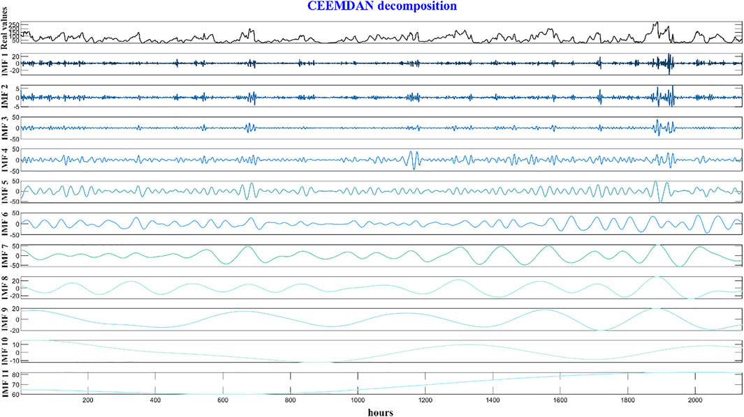
FIGURE 3. Pollutant series decomposed by CEEMDAN.

Calculate Sample and Fuzzy Entropy

Figure 3 clearly shows that the original data are decomposed by CEEMDAN to obtain different frequency components. From IMF1 to IMF11, the higher frequency of the IMF components indicates that each component contains more information and complexity. Therefore, we calculated the sample entropy and fuzzy entropy of each IMF separately to evaluate the complexity characteristics of different IMF time series. Table 2 shows that the frequency of the sequence from IMF1 to IMF11 gradually decreases, and the calculated sample entropy and fuzzy entropy also gradually decrease, which indicates that the complexity of the IMFs decreases.

TABLE 2

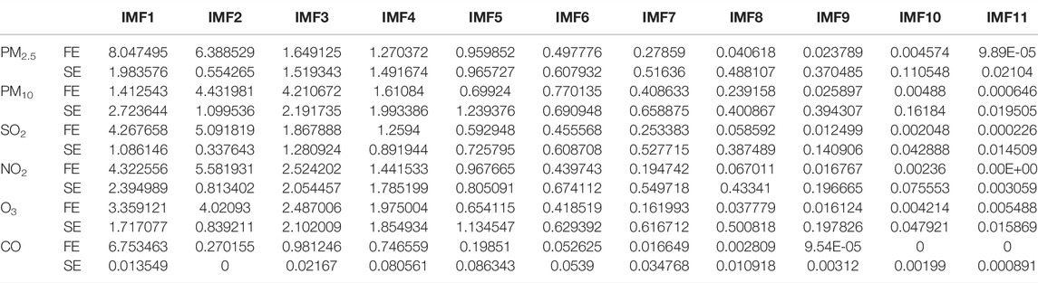
TABLE 2. Sample and fuzzy entropy of IMF.

Results of K-Means Cluster

Based on the entropy value results for each IMF component obtained from Table 2, a cluster analysis was implemented with K-means method. The clustering centers and groupings of each pollutant were obtained, as shown in Table 3. From the results in Table 3, we found that the 11 IMFs were clustered and reintegrated into 6 clusters. Each cluster is composed of IMF components with similar characteristics. The IMF components of each cluster are added together to form the final feature extraction datasets.

TABLE 3

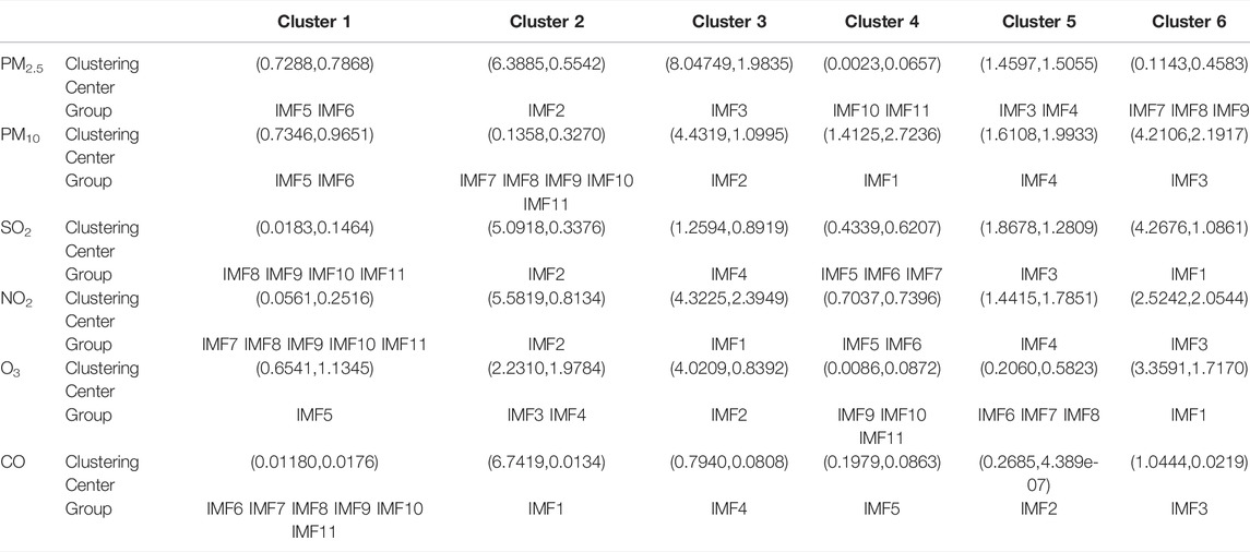
TABLE 3. Clustering centers and groupings of each pollutant by K-means.

Comparison of Forecasting Results

Comparison of Data Preprocessing Methods

In this experiment, the concentrations of six pollutants in Baoding were predicted and analyzed. This experiment compares the performance of three preprocessing models—Hampel-LSTM, CEEMDAN-LSTM, and our proposed model. Additionally, the evaluation criteria of MSE, MAE, and MAPE were used to measure the prediction performance of the models and the results are presented in Table 4. Boldly marked values are used to indicate the best values of the model in different evaluation metrics. Further discussion of the experimental results is as follows.

TABLE 4

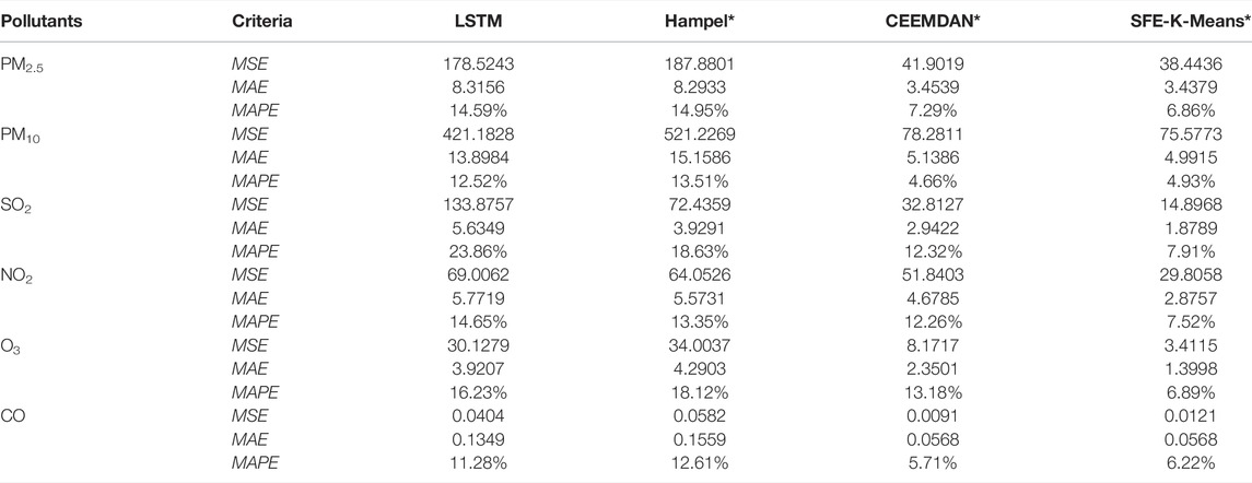
TABLE 4. Prediction performance of data preprocessing methods.

For the different data processing methods of the LSTM-based hybrid models, Table 4 shows that Hampel, CEEMDAN, and SFE-K-Means integrated with the same LSTM have obvious differences in prediction accuracy. However, compared with a single LSTM prediction model, the three hybrid models with signal processing tools—Hampel-LSTM(Hampel*), CEEMDAN-LSTM(CEEMDAN*), and SFE-K-Means-LSTM (SFE-K-Means*)—have better prediction performance. Therefore, it is safe to conclude that the use of mixed-preprecessing can significantly improve the data quality for the later hybrid model to obtain better prediction results. Subsequently, three hybrid prediction models based on different signal processing tools—Hampel*, CEEMDAN*, and SFE-K-Means*—were compared, and SFE-K-Means was found to have the highest prediction accuracy. For example, as for PM_2.5, the MAPE values of LSTM, Hampel*, CEEMDAN*, and SFE-K-Means* were 14.59, 14.95, 7.29, and 6.86%, respectively. Thus, LSTM integrated with SFE-K-Means outperforms the other data preprocessing models.

Comparison of Benchmark Methods

This experiment compares the performances of four single benchmark prediction models, including BPNN, ENN, and ELM. The models’ prediction performance was assessed using the MSE, MAE, and MAPE evaluation criteria; the results are presented in Table 5. The best results in the numerous evaluation metrics are emphasized by bold font. The results of the experiments are summarized below.

TABLE 5

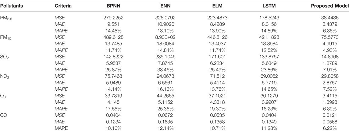
TABLE 5. Comparison of benchmark methods.

Table 5 clearly shows that LSTM seems to have more substantial predictive power than BPNN, ENN, and ELM. In the six pollutant concentration predictions, LSTM was superior to the other comparative models for all evaluation indexes. For example, the MAPE values for PM_2.5 via BPNN, ENN, ELM, LSTM and proposed model were 14.45, 18.10,13.90, 14.59 and 6.86%, respectively. The proposed model, which integrates SFE-K-Means with LSTM, results in the smallest MAE, MSE, and MAPE values, which says it should outperform the other benchmark methods to compare with. Notably, as a novel data preprocessing approaches, SFE-K-Means is critical for enhancing the forecast accuracy for environmental pollutant concentration.

Conclusion

The practical analysis and forecasting of pollutant concentrations are critical for environmental management and public health. Owing to the fluctuation and complexity of the pollutant data series, a novel mode decomposition-recombination technique is proposed to capture valuable information and characteristics. Six pollutant concentration series collected from Baoding were used as test cases to conduct the empirical study. Two experiments were implemented to compare the performances of the data preprocessing and forecasting methods, respectively. The evaluation criteria of MAE, MSE and MAPE were used to examine the prediction performance of the models. Based on the results of hourly pollutant concentration forecasting, some vital conclusions were drawn as follows. First, compared with Hampel*, CEEMDAN*, and SFE-K-Means*, the proposed SFE-K-Means* was found to have the highest prediction accuracy. Shown in Table 4 as for PM2.5, the MAPE values of LSTM, Hampel*, CEEMDAN*, and SFE-K-Means* were 14.59, 14.95, 7.29, and 6.86%, respectively. These errors explain that LSTM integrated with SFE-K-Means outperformed the other data preprocessing models. Second, compared with BPNN, ENN, and ELM, the proposed model, which integrates SFE-K-Means and LSTM, obtains lower values of MAE, MSE, and MAPE. This indicates that the proposed model can obtain the best forecasting performance among the compared models. Notably, the novel data preprocessing methods (SFE-K-Means) play an essential role in improving the prediction accuracy of environmental pollutant concentration.

In summary, the Hybrid model can change the traditional passive response of air quality management and provide strong technical support for urban air pollution early warning decisions, scientific air quality management, and regional joint prevention. Further, it can improve the level of air pollution control for air environment risk prevention.

Data Availability Statement

The original contributions presented in the study are included in the article/Supplementary material, further inquiries can be directed to the corresponding author.

Author Contributions

CN: Writing and Editing. ZN: Methodology. ZQ: Conceptualization and Writing-Reviewing. LW: Formal analysis. YL: Data curation and Visualization.

Funding

This work was supported by the National Social Science Foundation of China (Grant No. 17BTQ056) and the National Natural Science Foundation of China (Grant No. 72004086).

Conflict of Interest

The authors declare that the research was conducted in the absence of any commercial or financial relationships that could be construed as a potential conflict of interest.

Publisher’s Note

All claims expressed in this article are solely those of the authors and do not necessarily represent those of their affiliated organizations, or those of the publisher, the editors and the reviewers. Any product that may be evaluated in this article, or claim that may be made by its manufacturer, is not guaranteed or endorsed by the publisher.

References

Aksoy, A., Ertürk, Y. E., Erdoğan, S., Eyduran, E., and Tariq, M. M. (2018). Estimation of Honey Production in Beekeeping Enterprises from Eastern Part of Turkey through Some Data Mining Algorithms. Pjz 50, 2199–2207. doi:10.17582/journal.pjz/2018.50.6.2199.2207

CrossRef Full Text | Google Scholar

Allen, D. P. (2009). A Frequency Domain Hampel Filter for Blind Rejection of Sinusoidal Interference from Electromyograms. J. Neurosci. Methods 177, 303–310. doi:10.1016/j.jneumeth.2008.10.019

PubMed Abstract | CrossRef Full Text | Google Scholar

Bai, Y., Li, Y., Wang, X., Xie, J., and Li, C. (2016). Air Pollutants Concentrations Forecasting Using Back Propagation Neural Network Based on Wavelet Decomposition with Meteorological Conditions. Atmos. Pollut. Res. 7, 557–566. doi:10.1016/j.apr.2016.01.004

CrossRef Full Text | Google Scholar

Chen, L., and Pai, T.-Y. (2015). Comparisons of GM (1,1), and BPNN for Predicting Hourly Particulate Matter in Dali Area of Taichung City, Taiwan. Atmos. Pollut. Res. 6, 572–580. doi:10.5094/APR.2015.064

CrossRef Full Text | Google Scholar

Chen, W., Zhuang, J., Yu, W., and Wang, Z. (2009). Measuring Complexity Using FuzzyEn, ApEn, and SampEn. Med. Eng. Phys. 31, 61–68. doi:10.1016/j.medengphy.2008.04.005

PubMed Abstract | CrossRef Full Text | Google Scholar

Elbayoumi, M., Ramli, N. A., and Fitri Md Yusof, N. F. (2015). Development and Comparison of Regression Models and Feedforward Backpropagation Neural Network Models to Predict Seasonal Indoor PM2.5-10 and PM2.5 Concentrations in Naturally Ventilated Schools. Atmos. Pollut. Res. 6, 1013–1023. doi:10.1016/j.apr.2015.09.001

CrossRef Full Text | Google Scholar

Huang, K., Xiao, Q., Meng, X., Geng, G., Wang, Y., Lyapustin, A., et al. (2018). Predicting Monthly High-Resolution PM2.5 Concentrations with Random Forest Model in the North China Plain. Environ. Pollut. 242, 675–683. doi:10.1016/j.envpol.2018.07.016

PubMed Abstract | CrossRef Full Text | Google Scholar

Huang, N. E., Shen, Z., Long, S. R., Wu, M. C., Shih, H. H., Zheng, Q., et al. (1998). The Empirical Mode Decomposition and the Hilbert Spectrum for Nonlinear and Non-stationary Time Series Analysis. Proc. R. Soc. Lond. A 454, 903–995. doi:10.1098/rspa.1998.0193

CrossRef Full Text | Google Scholar

Li, C., and Zhu, Z. (2018). Research and Application of a Novel Hybrid Air Quality Early-Warning System: A Case Study in China. Sci. Total Environ. 626, 1421–1438. doi:10.1016/j.scitotenv.2018.01.195

PubMed Abstract | CrossRef Full Text | Google Scholar

Li, H., Wang, J., Li, R., and Lu, H. (2019). Novel Analysis-Forecast System Based on Multi-Objective Optimization for Air Quality Index. J. Clean. Prod. 208, 1365–1383. doi:10.1016/j.jclepro.2018.10.129

CrossRef Full Text | Google Scholar

Liu, C.-W., and Kang, S.-C. (2014). “A Video-Enabled Dynamic Site Planner,” in Computing in Civil and Building Engineering - Proceedings of the 2014 International Conference on Computing in Civil and Building Engineering, Orlando, Florida, June 23-25, 2014, 1562–1569. doi:10.1061/9780784413616.194

CrossRef Full Text | Google Scholar

Liu, H., and Chen, C. (2020). Prediction of Outdoor PM2.5 Concentrations Based on a Three-Stage Hybrid Neural Network Model. Atmos. Pollut. Res. 11, 469–481. doi:10.1016/j.apr.2019.11.019

CrossRef Full Text | Google Scholar

Liu, L., Breitner, S., Pan, X., Franck, U., Leitte, A. M., Wiedensohler, A., et al. (2011). Associations between Air Temperature and Cardio-Respiratory Mortality in the Urban Area of Beijing, China: A Time-Series Analysis. Environ. Health 10. doi:10.1186/1476-069X-10-51

PubMed Abstract | CrossRef Full Text | Google Scholar

Liu, Y., Zhang, S., Chen, X., and Wang, J. (2018). Artificial Combined Model Based on Hybrid Nonlinear Neural Network Models and Statistics Linear Models-Research and Application for Wind Speed Forecasting. Sustainability 10, 4601. doi:10.3390/su10124601

CrossRef Full Text | Google Scholar

Macqueen, J. (1967). “Some Methods for Classification and Analysis of Multivariate Observations,” in Proceedings of the fifth Berkeley symposium on mathematical statistics and probability, California, Berkeley, June 21-July 18, 1965, 281–297.

Google Scholar

Pandey, A., Brauer, M., Cropper, M. L., Balakrishnan, K., Mathur, P., Dey, S., et al. (2021). Health and Economic Impact of Air Pollution in the States of India: the Global Burden of Disease Study 2019. Lancet Planet. Health 5, e25–e38. doi:10.1016/S2542-5196(20)30298-9

PubMed Abstract | CrossRef Full Text | Google Scholar

Qi, Y., Li, Q., Karimian, H., and Liu, D. (2019). A Hybrid Model for Spatiotemporal Forecasting of PM2.5 Based on Graph Convolutional Neural Network and Long Short-Term Memory. Sci. Total Environ. 664, 1–10. doi:10.1016/j.scitotenv.2019.01.333

PubMed Abstract | CrossRef Full Text | Google Scholar

Riches, N. O., Gouripeddi, R., Payan-Medina, A., and Facelli, J. C. (2022). K-Means Cluster Analysis of Cooperative Effects of CO, NO2, O3, PM2.5, PM10, and SO2 on Incidence of Type 2 Diabetes Mellitus in the US. Environ. Res. 212, 113259. doi:10.1016/j.envres.2022.113259

PubMed Abstract | CrossRef Full Text | Google Scholar

Richman, J. S., Moorman, J. R., Randall, J., and Physi, M. (2000). Physiological Time-Series Analysis Using Approximate Entropy and Sample Entropy. Am. J. Physiology-Heart Circulatory Physiology 278, H2039–H2049. doi:10.1152/ajpheart.2000.278.6.H2039

PubMed Abstract | CrossRef Full Text | Google Scholar

Shang, Z., Deng, T., He, J., and Duan, X. (2019). A Novel Model for Hourly PM2.5 Concentration Prediction Based on CART and EELM. Sci. Total Environ. 651, 3043–3052. doi:10.1016/j.scitotenv.2018.10.193

PubMed Abstract | CrossRef Full Text | Google Scholar

Tang, J. W., Lai, F. Y. L., Nymadawa, P., Deng, Y.-M., Ratnamohan, M., Petric, M., et al. (2010). Comparison of the Incidence of Influenza in Relation to Climate Factors during 2000-2007 in Five Countries. J. Med. Virol. 82, 1958–1965. doi:10.1002/jmv.21892

PubMed Abstract | CrossRef Full Text | Google Scholar

Tessum, C. W., Hill, J. D., and Marshall, J. D. (2015). Twelve-month, 12 Km Resolution North American WRF-Chem v3.4 Air Quality Simulation: Performance Evaluation. Geosci. Model Dev. 8, 957–973. doi:10.5194/gmd-8-957-2015

CrossRef Full Text | Google Scholar

Wang, D., Wei, S., Luo, H., Yue, C., and Grunder, O. (2017a). A Novel Hybrid Model for Air Quality Index Forecasting Based on Two-phase Decomposition Technique and Modified Extreme Learning Machine. Sci. Total Environ. 580, 719–733. doi:10.1016/j.scitotenv.2016.12.018

PubMed Abstract | CrossRef Full Text | Google Scholar

Wang, P., Zhang, H., Qin, Z., and Zhang, G. (2017b). A Novel Hybrid-Garch Model Based on ARIMA and SVM for PM 2.5 Concentrations Forecasting. Atmos. Pollut. Res. 8, 850–860. doi:10.1016/j.apr.2017.01.003

CrossRef Full Text | Google Scholar

Wu, L., and Zhao, H. (2019). Using FGM(1,1) Model to Predict the Number of the Lightly Polluted Day in Jing-Jin-Ji Region of China. Atmos. Pollut. Res. 10, 552–555. doi:10.1016/j.apr.2018.10.004

CrossRef Full Text | Google Scholar

Wu, Z., and Huang, N. E. (2009). Ensemble Empirical Mode Decomposition: A Noise-Assisted Data Analysis Method. Adv. Adapt. Data Anal. 01, 1–41. doi:10.1142/S1793536909000047

CrossRef Full Text | Google Scholar

Xu, Y., Yang, W., and Wang, J. (2017). Air Quality Early-Warning System for Cities in China. Atmos. Environ. 148, 239–257. doi:10.1016/j.atmosenv.2016.10.046

CrossRef Full Text | Google Scholar

Yahya, K., Zhang, Y., and Vukovich, J. M. (2014). Real-time Air Quality Forecasting over the Southeastern United States Using WRF/Chem-MADRID: Multiple-Year Assessment and Sensitivity Studies. Atmos. Environ. 92, 318–338. doi:10.1016/j.atmosenv.2014.04.024

CrossRef Full Text | Google Scholar

Yan, R., Liao, J., Yang, J., Sun, W., Nong, M., and Li, F. (2021). Multi-hour and Multi-Site Air Quality Index Forecasting in Beijing Using CNN, LSTM, CNN-LSTM, and Spatiotemporal Clustering. Expert Syst. Appl. 169, 114513. doi:10.1016/j.eswa.2020.114513

CrossRef Full Text | Google Scholar

Yan, X., and Enhua, X. (2020). “ARIMA and Multiple Regression Additive Models for PM2.5 Based on Linear Interpolation,” in Proceedings - 2020 International Conference on Big Data and Artificial Intelligence and Software Engineering, ICBASE, Bangkok, Thailand, Oct. 30 2020 to Nov. 1 2020, 266–269. doi:10.1109/ICBASE51474.2020.00062

CrossRef Full Text | Google Scholar

Yuchi, W., Gombojav, E., Boldbaatar, B., Galsuren, J., Enkhmaa, S., Beejin, B., et al. (2019). Evaluation of Random Forest Regression and Multiple Linear Regression for Predicting Indoor Fine Particulate Matter Concentrations in a Highly Polluted City. Environ. Pollut. 245, 746–753. doi:10.1016/j.envpol.2018.11.034

PubMed Abstract | CrossRef Full Text | Google Scholar

Zadeh, L. A. (1965). Fuzzy Sets. Information and Control 8, 338–353. doi:10.1016/S0019-9958(65)90241-X

CrossRef Full Text | Google Scholar

Zhang, L., Lin, J., Qiu, R., Hu, X., Zhang, H., Chen, Q., et al. (2018). Trend Analysis and Forecast of PM2.5 in Fuzhou, China Using the ARIMA Model. Ecol. Indic. 95, 702–710. doi:10.1016/j.ecolind.2018.08.032

CrossRef Full Text | Google Scholar

Zhang, S., Liu, Y., Wang, J., and Wang, C. (2019). Research on Combined Model Based on Multi-Objective Optimization and Application in Wind Speed Forecast. Appl. Sci. 9, 423. doi:10.3390/app9030423

CrossRef Full Text | Google Scholar

Zhou, Q., Jiang, H., Wang, J., and Zhou, J. (2014). A Hybrid Model for PM 2.5 Forecasting Based on Ensemble Empirical Mode Decomposition and a General Regression Neural Network. Sci. Total Environ. 496, 264–274. doi:10.1016/j.scitotenv.2014.07.051

PubMed Abstract | CrossRef Full Text | Google Scholar

Zhu, S., Lian, X., Wei, L., Che, J., Shen, X., Yang, L., et al. (2018). PM2.5 Forecasting Using SVR with PSOGSA Algorithm Based on CEEMD, GRNN and GCA Considering Meteorological Factors. Atmos. Environ. 183, 20–32. doi:10.1016/j.atmosenv.2018.04.004

CrossRef Full Text | Google Scholar