 Yuan Gao
 Lidu Shen
 Rongrong Cai1
 Fenghui Yuan
 Jiabing Wu
- 1CAS Key Laboratory of Forest Ecology and Management, Institute of Applied Ecology, Chinese Academy of Sciences, Shenyang, China
- 2College of Resources and Environment, University of Chinese Academy of Sciences, Beijing, China
- 3Department of Soil, Water, and Climate, University of Minnesota, Saint Paul, MN, United States
- 4Department of Geography, Nipissing University, North Bay, ON, Canada
Forest canopy closure affects snow processes by changing the redistribution of snowfall, snow interception, accumulation, sublimation, and melt. However, how the forest closure impacts snow processes at different periods has not been well explored. We conducted 3-year measurements of snow density and depth and carried out snow process calculations (i.e., interception, sublimation, and snowmelt) from 2018 to 2021 in four mixed forests with different canopy closures and an open site in the Changbai Mountains, northeast China. We found that the snow density of the five study sites varied greatly (0.14–0.45 g/cm3). The snow depth (SD) at four mixed forests sites was smaller than that of the nearby open site. The SD decreased as the forest canopy closure increased. Additionally, the forest interception effect increased with the canopy closure and decreased as the snowfall intensity increased. The total interception efficiency of the four mixed forests in normal snow years changed from 34% to 73% and increased with forest canopy closure. The averaged sublimation rate (Ss) and snowmelt rate (Sr) of the four mixed forests varied during different periods of snow process. The Ss was 0.1–0.4 mm/day during the accumulation period and 0.2–1.0 mm/day during the ablation period, and the Sr was 1.5–10.5 mm/day during the ablation period. There was a good correlation between Ss, or Sr, and canopy closure, but interannual variation was observed in the correlation. The mean values of the effect of the four mixed forests on understory SWE (snow water equivalent) over the 3 years ranged from −45% to −65%. Moreover, the impact effect was correlated with the forest canopy closure and enhanced with the canopy closure. This study provided more scientific information for studies of snow cover response to forest management.
1 Introduction
Snow cover and its changes are important as they alter the soil temperature and soil water content in forestland (Chang et al., 2014; Maurer and Bowling, 2014; Lyu and Zhuang, 2018), and they also impact the climate feedback in forestland (Henderson et al., 2018; Krinner et al., 2018). Forest cover, annual snowfall, elevation, winter temperature, and snowfall form are the main factors affecting forest snow (Lopez-Moreno and Stahli, 2008; Lundquist et al., 2013; O'Gorman, 2014). A previous review study of 65 sites by Varhola et al. (2010) showed that forest cover was the most important factor affecting the forest snow process and that forest cover changes could explain 57%–72% of the relevant variation in the forest snow process. This is mainly because the forest canopy changes the amount and spatial distribution of snow on the ground through canopy interception at the local scale. In the meantime, the canopy structure altered the amount of the long-wave and short-wave radiation input to the understory snow surface, which in turn affected the snow surface energy balance and ultimately controlled the forest snow accumulation and ablation process (Ellis et al., 2010; Musselman et al., 2012; Roth and Nolin, 2017). Thus, the snow processes in the understory would be altered synchronously with changes in forest structure. Many studies have reported the effect mechanisms of forest structure changes on snow processes, such as deforestation (Schelker et al., 2013; Revuelto et al., 2016; Krogh et al., 2020), fire disturbance (Maxwell et al., 2019; Schwartz et al., 2020), insect pests (Pugh and Gordon, 2013; Perrot et al., 2014), and avalanche disturbances (Bebi et al., 2009; Casteller et al., 2018). Although the study of the mechanistic processes of forest snow is the key to reveal the relationship between forest structural changes and the response of snow processes, there are still many limitations in the application and extension of the results of previous studies to other regions, such as northeastern China. First, forest snow processes are localized and strongly dependent on forest structure characteristics, and there are obvious regional differences in the two elements affecting forest structure (regional climate and forest disturbance patterns). Second, the multiple forest structure parameters (e.g., LAI, forest cover, and canopy cover) and abundant research methods (e.g., modeling method, remote sensing method, and snow survey method) also make the research results low comparability with each other. Again, due to fewer studied cases in northeastern China, there is a lack of comprehensive understanding of the variation of forest snow sub-processes (interception, sublimation, and ablation) in different periods and years in this region. Thus, these constrained our understanding of snow processes in the widely distributed mixed forests in northeastern China and also limited the follow-up studies on the simulation and prediction of the effects of different climate change scenarios and different forest management methods on snow processes in the future.
The influence of forest structure on snow processes is basically a small-scale interaction process, and the interaction between forest and snow is strongly dependent on the factors such as forest structural characteristics, climate type, altitude factors, and the atmospheric conditions of winter. Some studies have also quantified the effects of forests on snow processes using the open area and forest normalized contrast method (Veatch et al., 2009; Varhola et al., 2010; Broxton et al., 2015). However, most of these studies were conducted in Europe and North America and in other forest regions with large amounts of snowfall (i.e., SnowMIP2 sites). There are few studies on the impact of a mixed forest structure on snow cover in northeast China. In particular, the widespread natural mixed forests in this region have experienced cutting at multiple intensities of 20%, 40%, 80% and 100% since the 1980s, and forest structure elements, such as canopy closure, have changed greatly, which also caused complex changes in the forest snow processes. It is difficult to directly use the findings from previous studies regarding the effects of snow processes on changes under the forest closure gradient to reveal the interaction process and mechanism between forest and snow in northeast China. How the changes in the canopy closure affected forest snow regime in this region is still unclear.
Changes in forest structure and their impacts on snow processes are complicated. A selection of appropriate forest structure indicators to quantify the impact is particularly critical, but the diversity of indicators and methods has instead limited research expansion. A variety of forest structure indicators have been used to reveal the impact of forests on snow processes, such as forest cover (Varhola et al., 2010; Pomeroy et al., 2012; Varhola and Coops, 2013), canopy cover (Pomeroy et al., 2002), leaf area index (Gelfan et al., 2004; Woods et al., 2006; Rutter et al., 2009; Lendzioch et al., 2019), and canopy closure (Broxton et al., 2021). In the meantime, as technology continues to progress, various methods have been applied comprehensively, such as forest snow sampling survey (Watson et al., 2006; Parajuli et al., 2020), snow model simulation (Pomeroy et al., 2007; Rutter et al., 2009; Krinner et al., 2018; Napoly et al., 2020), statistical modeling (López-Moreno and Nogués-Bravo, 2006), snow remote sensing (Zhang et al., 2010; Frei et al., 2012; Hojatimalekshah et al., 2021), LiDAR technology (Harpold et al., 2014; Broxton et al., 2021; Russell et al., 2021), UAV remote sensing (Lendzioch et al., 2019), and delayed photography (Parajka et al., 2012; Dong and Menzel, 2017). When studying forest snow process in specific areas, the most appropriate method needs to be selected and balanced, as each method has certain advantages and limitations. Snow surveys need to take into account a variety of heterogeneous landscapes and survey frequency and strategy (Watson et al., 2006), and these factors can result in higher implementation costs. Snow model method has the problems of a coarse resolution and the simplification of the interaction processes between forest and snow (Broxton et al., 2021), restricting the ability of existing models to quantify effects of the forest canopy structure changes on snow processes. For example, Rutter et al. (2009) and Krinner et al. (2018) only focused on the accurate simulation of snow processes in specific forests and in adjacent open areas when conducting SnowMIP2 and ESM-SnowMIP studies. In addition, snow remote sensing products cannot be widely used to complex forest areas because of their high cost and limited snow capture accuracy (Rutter et al., 2009; Steele et al., 2017; Jacobs et al., 2021). Therefore, previous studies on the interaction between forest and snow have some deficiencies in terms of expanding their application to other regions (i.e., northeast China), due to the diversity of forest structure parameters, the different survey strategies and models selected, and the specific climate and forest types in other regions.
In addition, the impact of forests on snow processes varied over different periods and forest cover. An integrative study of 65 sites in North America and Europe by Varhola et al. (2010) showed that forest cover may have both positive and negative impacts on snow processes. One reason for this is that the impact of forests on the snow process is a result of the continuous or cumulative impact on multiple sub-processes (snow interception, snow sublimation, snow metamorphism, and snow ablation) after every single snowfall event. Though many previous studies have investigated the sub-processes of forest snow, such as canopy interception (Stähli et al., 2009), snow sublimation (Montesi et al., 2004; Li et al., 2013; Li et al., 2016; Sexstone et al., 2018), and snow ablation (Burles and Boon, 2011), in single forest types, the effects of forest on different sub-processes varied not only in magnitude but also among the periods of the related sub-processes in question, and the total effect was the combined result of continuous multiple snow sub-processes. Few studies have addressed whether there are differences in the effects of forest structure in different periods and years. Likewise, random effects caused by focusing on a single snow sub-process or specific period are inevitable, and it is difficult to reflect the comprehensive impact of forest on the entire snow process. This makes previous studies lack representation on different snow years. Therefore, it is particularly important to comprehensively or quantitatively evaluate the impact of forest structure on snow process throughout the whole snow season. The effects of forest structure or its change on snow process need more in-depth or quantitative investigation.
To reveal this impact effect comprehensively and provide more region-specific information, we conducted a three-year study of the snow processes at four forest sites with different levels of forest canopy closure and at a nearby open site in the Changbai Mountains, northeast China. The snow characteristics (snow density and depth) and snow sub-processes (snow interception, snow sublimation rate, and snowmelt rate) were measured. We selected the forest canopy closure as a forest structure parameter to study the impact of the forest on snow processes and analyzed the relationships of these sub-processes with forest canopy closure. The purpose is to provide the characteristics and distribution regularity of snow properties in the forest area, which is beneficial for developing a forest snow model based on forest closure. The sections of this article are as follows. Section 2 provides information about the forests in the study area, the investigation methods to determine forest structure and snow cover characteristics, and the calculation methods of snow processes. Section 3 compares the snow forest cover characteristics (i.e., snow density and snow depth) with canopy closure, analyzes the relationship between forest canopy closure and snow sub-processes, and quantifies the impact of each forest on the different snow processes. Finally, a discussion and conclusions are provided in Sections 4 and 5, respectively.
2 Study Area and Methods
2.1 Study Area
The study area (42.29°–42.57°N, 127.75°–128.13°W) is located in the Changbai Mountains, northeast China (Figure 1). It has a temperate continental climate with an annual average temperature of 3.6°C and annual precipitation of 735 mm (Li et al., 2016). The average temperature for winter is −14°C, and the annual snowfall is about 133 mm, which accounts for 18.2% of the annual precipitation. Forest snow cover generally lasts from November to April. The region has a distribution area of temperate natural coniferous and broad-leaved mixed forest, and this type of mixed forest is typical in northeast China. After decades of different management methods (protection and selective cutting), the natural mixed forests and multi-type forests have been disturbed by human activities. The main tree species in these natural mixed forests are Pinus koraiensis, Tilia amurensis, Fraxinus mandshurica, Quercus mongolica, Acer mono, and White birch. Canopy height varies between 15 and 30 m. The stand density can reach 560 stems/ha (stem diameter > 8 cm), and the maximum leaf area index can be 6.0 (Wu et al., 2012). The soil type is montane dark brown and was developed from volcanic ash (Guan et al., 2006).
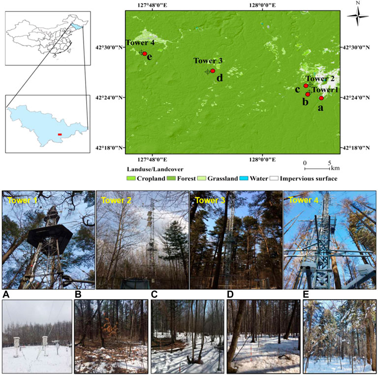
FIGURE 1. The location of the study area (top row), pictures of the open-path eddy covariance (EC) flux system (middle row), and pictures of the plots in the study area in the Changbai Mountains, northeastern China (bottom row). The EC flux system corresponds to the plots one by one: Tower 1-b, Tower 2-c, Tower 3-d, and Tower 4-e. The letters in top and bottom rows correspond to different land types and disturbance intensities: (A) the open site (OS); (B) the natural mixed forest (NMF); (C) the high-intensity cutting mixed forest (HCF); (D) the moderate-intensity cutting mixed forest (MCF); and (E) the low-intensity cutting mixed forest (LCF).
Four plots of mixed forests with different cutting intensities were selected (0, 20%, 40%, and 100%), from a similar altitude (750 m), with a low slope and at same slope orientation, and having a forest stand size of 40 m × 40 m. The plots comprised a natural mixed forest (NMF) without cutting, low-intensity cutting mixed forest (LCF, 20%), moderate-intensity cutting mixed forest (MCF, 40%), and high-intensity cutting mixed forest (HCF, 100%) (Figure 1). These four forests formed gradually after harvesting the original natural mixed forests using different cutting intensities 30 years ago. A nearby open site (OS) was used as a contrast plot or control to study the effect of forest canopy structure on snow processes. Field conditions and forest information of the five plots are shown in Figure 1 (bottom row) and Table 1.
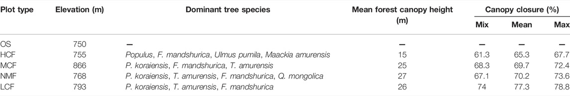
TABLE 1. Detailed information of forest plots.
2.2 Field Observations
2.2.1 Meteorological Observations
Meteorological data were collected from the open site meteorological station (Figure 1A). The main meteorological elements included temperature and humidity (using the HMP45C, Vaisala, Helsinki, Finland), wind speed (A100R, Vector Instruments, Denbighshire, United Kingdom), net radiation (CNR 4, Kipp & Zonen, Delft, the Netherlands), and precipitation (Rain Gauge 52203, Young, Traverse City, MI, United States). Surface snow depth was observed by delayed photography (CC5MPX, Campbell, United States). Each meteorological element was recorded at half-hour intervals. The daily meteorological data were obtained from the conversion of half-hour intervals data.
2.2.2 Snow Surveys
Snow surveys were conducted at five study sites (four forested and one open site) from November to April of each year during 2018–2021 (Figure 2). Snow survey frequency was once weekly to bi-weekly according to the snowfall in the accumulation period, and the frequency was increased to every 3–5 days depending on the accessibility of mountain roads in the ablation period. The investigation strategy to determine the snow depth at the stand level is shown in Figure 2A. Each forest plot (40 m × 40 m) was divided into sub-grids of six rows and six columns, and a snow ruler was placed in each sub-grid (Figure 2A), meaning that each plot had a total of 36 snow depth rulers distributed within it. The positions of the snow rulers were further adjusted according to the distribution positions of the tree trunks and forest gaps in each sub-grid so that each ruler could represent the approximate average snow depth value of the sub-grid as accurate as possible. To reduce the disturbance of the forest snow caused by human activities, we used a telescope to observe the snow depth rulers remotely. The snow depth at the five sites was measured by using fixed snow rulers (Figure 3A). A red and white alternate ruler was fixed on the ground, and the minimum accuracy was 1 cm, and the maximum value was 80 cm (Figure 3A).
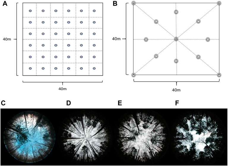
FIGURE 2. Investigation strategy maps of the forest snow depth (A), investigation location of canopy closure at the stand level (B), and forest hemisphere images (bottom row, C, D, E, and F). The circles in (A) represent the location of snow rulers, and the circles in (B) represent image captures in the forest plot. Four forest hemisphere images (bottom row): (C) high-intensity cutting mixed forest (HCF); (D) moderate-intensity cutting mixed forest (MCF); (E) natural mixed forest (NMF); (F) low-intensity cutting mixed forest (LCF).
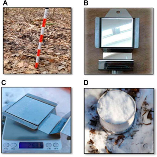
FIGURE 3. Investigation methods to determine snow cover characteristics: (A) snow depth ruler, (B) rectangular snow box cutter, (C) weight to determine the snow mass, and (D) snow sublimation rate measurement method.
The snow density was calculated using the weighing wedge snow density box cutter method (5 cm × 4.54 cm × 4.2 cm, 235.6 g) (Figure 3B). This method had been applied in snow surveys and the performance of this device was evaluated by Hao et al. (2021). In the snow field survey, the method was used together with a high rate of accuracy (0.1 g), low-temperature resistance (−40°C to 40°C), and a waterproof electronic scale (Figure 3C). Before the snow sample was taken, a vertical snow profile was excavated first, and the profiles were layered at 10 cm intervals. Then, the long end of the density device was inserted into the corresponding layer in the same direction as the vertical snow profile to collect the snow samples. After the snow filled up the inner space of the box, the box was removed, the cover was put on top of it, and it was finally placed on the electronic scale for weighing (Figure 3C).
2.2.3 Eddy Covariance Measurement of Snow Sublimation
Near each forest plot, there was an open-path eddy covariance (EC) flux system installed on the meteorological tower in each area to take long-term meteorological records (Figure 1, Tower 1–4). The EC principle uses the deviation in vertical wind speed and the deviation of water vapor concentration to calculate the water vapor flux (ET) as follows:
where ET is the water vapor flux (kg/m2∙s), ρd is the air density (kg/m3), w′ is the vertical wind speed (m/s), and s′ is the dry mole fraction of the gas in water (kg/kg). The overbar represents an average value over 30 min.
The water vapor flux was pre-processed using EddPro-7.0.2 software and post-processed using Tovi™ software. A missing threshold of pre-processed raw data was set to 10%, and the vertical wind speed threshold was set to 3 m/s. After that, we used the double coordinate rotation method proposed by Wilczak et al. (2001) to correct the vertical wind speed and used the Webb-Pearman-Leuning (WPL) correction developed by Webb et al. (1980) to correct the water vapor flux, which was caused by the density effect. Next, we applied the recommended tools from Tovi™ to execute gap-filling (Reichstein et al., 2005), data screening, spectral corrections, and energy balance residual correction (Mauder et al., 2013; Charuchittipan et al., 2014; De Roo et al., 2018). Finally, we converted half-hour data of water flux into day flux.
2.2.4 Forest Structure Measurements
The forest structure parameters (i.e., dominant species, tree height, and canopy closure) were measured and collected. We combined the relative height of the tower to obtain the height information of the main forest species and investigated the dominant species in each plot. Detailed information of forest plots was summarized in Table 1.
Hemispherical Canopy Photography is an indirect optical technique that has been widely used to determine forest canopy structure. The canopy openness of the forest plots was obtained by hemispherical photography based on the optical imaging principle (device information: EOS 5D + EF, 8–15 mm Fisheye, Canon Inc., Japan). An upward-looking method was used to obtain hemispherical images during the winter period when the canopy structure parameters were stable (Figure 2). In each forest plot (40 m × 40 m), a photographing route along the four sides and along the diagonal of the plot was adopted (Figure 2B). The photographing positions were placed in this way: four at the four corners of the square forest plot, one at the plot center, and eight around the center stretching out in eight directions, creating a total of 13 images for each plot (Figure 2B). The images data were analyzed by using the Gap Light Analyzer (GLA) software and the calculation methods by Frazer et al. (1999). The canopy closure (θ) was calculated using the formula: θ = 1 - canopy openness.
2.3 Calculation Methods
2.3.1 Standardizing Snow Depth
The large distance between the four forest plots (25 km) from east to west (Figure 1) may lead to spatial variation in snowfall, so we standardized the snow depth. After multiple snow surveys, we found that the snowfall near plots MCF and LCF had slightly higher snow depth than that in the reference site OS. We synchronously observed the snow depth of the open space near the LCF and found that the ratio between them remained approximately stable over a long period of time. Here, we assumed that the temporal changes in the snow cover caused by wind blowing and snow sublimation in two open areas (OS and the open space near LCF) with similar surface environments were mostly equal. Therefore, the ratio coefficient (α) for the annual snowfall in the two areas was equal to the snow depth ratio in two open areas.
Snowfall was the most important factor in controlling the forest snow depth. To compare the influence of the forest on snow depth under the conditions of unified snowfall, this coefficient was further used to uniformly adjust the measured snow depths of the MCF and LCF. The correction method is as follows:
where P1 is the snowfall observed in the OS (Figure 1A), P2 is the snowfall in the open area near the MCF and LCF, SD is the adjusted or standardized snow depth, SDmeasured is the measured snow depth from survey, and α is the adjusting coefficient. According to the regional snowfall data from the two regions over the three-year period (2018–2019, 2019–2020, and 2020–2021), the coefficients α are α1 = 0.65, α2 = 0.63, and α3 = 0.62, for each year, respectively.
2.3.2 Calculation of Snow Density and Snow Water Equivalent
Snow density sampling at a sampling point was carried out for each layer of the snow profile and repeated on each layer three times. Finally, the density of snow for a sample was calculated as follows:
where ρi is the density corresponding to a layer (g/cm3), m1 is the total weight of the box (g), m2 is the total mass of the empty box (g), and v is the internal volume (cm3). The average snow density of the snow profile was calculated as follows:
where ρ is the average density (g/cm3) and di is the snow depth of the corresponding layer (cm).
The snow water equivalent (SWE) and standard deviation (σ) at the forest stand scale were calculated as follows:
where SWE is the snow water equivalent (mm), SD is the average snow depth at the stand scale obtained by in situ snow depth surveys (n = 36 for each plot) (cm), and σ is the standard deviation for the survey samples within a plot.
2.3.3 Calculation of Canopy Snow Interception Coefficient
The interception coefficient was calculated for individual snowfall event by using variations in the snow depth before and after a single forest snowfall, at the forest site (ΔSDF) and at the open site (ΔSDO). They were observed using the time-lapse photography approach, which has been widely applied in forest snow studies (Garvelmann et al., 2012; Parajka et al., 2012; Dong and Menzel, 2017; Dong, 2018). The interception coefficient (CIE) of forest canopy was calculated as follows:
where ΔSDO and ΔSDF are the variations in snow depth in the open site and in the forest site for every single snowfall event, and they were measured in the open site (OS) and forest plots at three locations in each plot simultaneously, respectively.
The cumulative value of the forest canopy interception coefficient (Ic) over the whole snow season or the winter period was calculated as follows:
where Ic is the cumulative interception coefficient, ∆SDiO-∆SDiF is the canopy interception of a single snowfall event i, the sum is the accumulated interception depth of the entire winter (cm), and Psnowfall is the total snow depth (cm).
2.3.4 Calculation of Snow Sublimation by the Weighing Measurement Method
The snow sublimation in the open site (OS) was measured by the continuous daily weighing snow evaporator method (Figure 3D). Three circular cylindrical tubes that were 20 cm in diameter and made of white PVC plastic material were used as in situ snow collection device and placed in the OS site for the duration of the snow season. The height of the cylinder was able to be adjusted according to the depth of the external snow, and the connecting ring was used to increase or reduce the height of the cylinder to avoid snow exchange in the horizontal direction inside and outside of the weighing cylinder, as well as to control the disturbance caused by frequent manual measurements and to ensure the stability of the snow sample in the cylinder. The cylinder was weighed at 08:00, 12:00, and 16:00 each day, and the weight change from 16:00 on the previous day to 16:00 on the current day was measured as the snow sublimation amount of the day. The daily sublimation of snow in the OS was calculated as follows:
where ET is the snow sublimation (mm/day); M1 and M2 are the weights of the cylinder for the previous day (16:00) and for the present day (16:00) (g); P is the snowfall occurring within the weighing interval, which is measured by other separate empty cylinders for the weighting measurement (g); ρw is the liquid density of water (1.0 g/cm3); D is the diameter of the snow measuring cylinder (20 cm); and π is the circular rate constant (3.14).
2.3.5 Calculation of Snowmelt Rate by the Water Balance Method
To evaluate the impact of forests on the items of the snow water balance, we calculated the water balance during the snow melting period as follows:
where QSWE, QSnowfall, QE↑, and QS are the variation in the surface snow water equivalent during the melting period, snowfall accumulated on the snow surface, the snow sublimation, and the loss of snow via snowmelt which was converted into liquid water, respectively (QSWE is obtained through snow surveys, and QSnowfall is snowfall accumulation for each plot during the ablation period. QSnowfall represents penetrating snow in forests, which is obtained from time-lapse photography of snow depths under the forest and calculated by Eq. 6). It is noted that no rain-on-snow events were observed during the snow ablation periods in 3 years. QS is the loss of snow converted into liquid water in the snow layer during the ablation period and is estimated from Eq. 11. QE↑ is the snow sublimation and it is the total amount water flux returned to the atmosphere in the form of sublimation. Therefore, the value (QE↑) is the sum of the sublimation under the forest and the snow sublimation of the forest canopy which was calculated using the EC method.
In some previous studies for estimating snow water equivalent, the snow melting was calculated from meteorological data with empirical or energy-based methods [e.g., Yao et al. (2012); Yao et al. (2018)]. In our present study, the snow melting was calculated through the water balance equation (Eq. 11), as all other items were obtained by field measurements. The daily snowmelt rate (Sr) was calculated as follows, by similarly using water balance:
where Sr is the daily rate of snowmelt (mm/day), and
2.3.6 Quantification of the Effects of Forest on the Snow Process
To ensure that the impacts that forests have on snow processes are comparable across different years and different forest types, a forest and open site comparison method was used to calculate the effect value (E). This normalization method for different forest snow data was based on the effect value calculated by the reference point OS, and a method similar to that proposed by Varhola et al. (2010) was adopted, which quantified the effect uniformly over the whole season (accumulation and ablation periods). The E was calculated as follows:
where SWEForest is the average snow water equivalent (SWE) of each forest type at the plot scale, SWEOpen site is the average snow water equivalent (SWE) of the open site (OS), which is calculated by Eq. 6 based on the snow surveys. E is the effect value, representing the average value calculated after multiple surveys throughput the entire survey period for each winter. A negative value indicates that there is a decreasing impact of the forest on the understory SWE (snow water equivalent), while a larger absolute value indicates a stronger impact of the forest on the understory SWE.
3 Results
3.1 Meteorological Characteristics During the Study Period
The meteorological conditions varied throughout the whole snow cover period (Figure 4). The rapid shift between snow accumulation and ablation periods is strongly controlled by meteorological factors, such as snowfall, net radiation, air temperature, and other factors. According to various characteristics of meteorological elements (average temperature, net radiation, and the maximum snow depth) in the open area OS, we found that the date of the maximum snow depth appeared when the daily-average temperature was reaching 0°C in our research area, indicating the air temperature was the most important factor controlling the shift from accumulation to ablation. Therefore, the date of the maximum snow depth was used to divide the whole snow process into two periods, the Ac period and the Ab period. The maximum snow depth was reached on 20 February 2019, 20 March 2020, and 15 February 2021, respectively, for the three winter seasons. The maximum snow depth in the OS was 25 cm (2018–2019), 63 cm (2019–2020), and 27 cm (2020–2021), respectively. Overall, both air temperature (Ta) and net radiation (Ra) are the main input sources of snow ablation energy, and their values varied at different periods, which together regulate the transition between the Ac and Ab periods. Over the 3 years, the average of Ta in Ac was about −11.2°C (2018–2019), −9.1°C (2019–2020), and −12°C (2020–2021), and the average of Ra in Ac was 7.75 MJ/m2 (2018–2019), 6.76 MJ/m2 (2019–2020), and 6.6 MJ/m2 (2020–2021), respectively. During the three Ab periods, the average of Ta increased to −2.2°C (2018–2019), 1.86°C (2019–2020), and −6°C (2020–2021), and the average of Ra increased to 13.1 MJ/m2 (2018–2019), 18.8 MJ/m2 (2019–2020), and 9.95 MJ/m2 (2020–2021). The average values of Ta and Ra in the Ac period were lower than those in the Ab period.
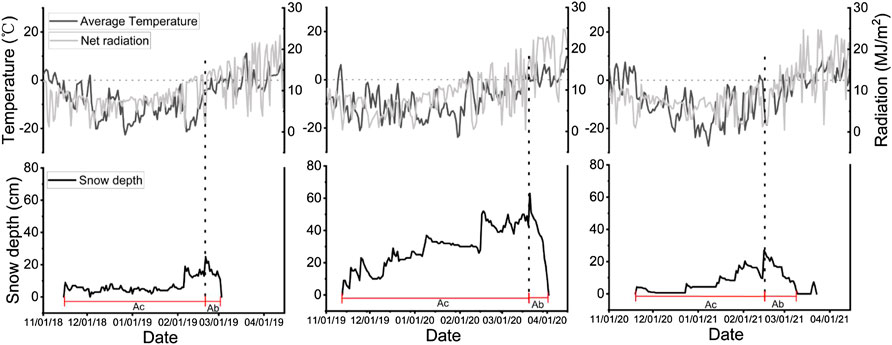
FIGURE 4. Characteristics of meteorological conditions during snow accumulation and ablation processes in the open area OS, for each of the three winter seasons. The maximum snow depth appeared near the 0°C air temperature and was used as the dividing date for two periods, where Ac is the accumulation period that occurred before the maximum snow depth date, and Ab is the ablation period.
The changes in Ta and Ra during the Ab period affected the pattern of snow melting and thus strongly controlled the duration of the snow. Although the maximum snow depth in 2019–2020 (63 cm) was far greater than that in the other 2 years (Figure 4 middle column), the multi-day average of Ta and Ra during the Ab period remained the highest at 1.86°C and 18.8 MJ/m2; thus, fast ablation was observed during this snowmelt period. The ablation curve was also relatively steep, and the Ab period lasted just 13 days. However, the maximum snow depth in 2020–2021 was only 27 cm in the OS (Figure 4 right column). The multi-day average of Ta and Ra in the Ab period were only −6°C and 9.95 MJ/m2 and showed a slow increasing trend. As a result, the snow had showed a slow ablation, and the Ab period lasted for the longest amount of time: 23 days (2020–2021). Correspondingly, there were 11 (2018–2019), 13 (2019–2020), and 23 (2020–2021) snow ablation days for the 3 years. Thus, the ablation pattern and ablation duration in the Ab period were mainly controlled by the Ta and Ra. The higher the values of Ta and Ra, the faster the ablation rate, and correspondingly, the shorter the ablation period.
3.2 Variations in Snow Density and Snow Depth at Five Sites
The snow density (ρ) varied largely with the day of winter (DOW) within the different land types: between 0.14 and 0.45 g/cm3 at the five sites (Figure 5). Throughout the three winters, the ρ of the five sites in the Ac period was smaller than that in the Ab period, and ρ increased with the DOW. The ρ during the Ac period was about 0.14–0.35 g/cm3, while during the Ab period, the ρ of the five sites all showed an increasing trend, varying between 0.35 and 0.45 g/cm3. The relationship between ρ and DOW of the five sites showed the best (R2 = 0.84) linear correlation in 2019–2020, and the correlation results in 2018–2019 (R2 = 0.34) and in 2020–2021 (R2 = 0.45) were relatively weaker. Changes in meteorological conditions also affected the relationship between ρ and DOW. The annual snowfall in 2019–2020 was close to the average annual snowfall in the region for many years, but 2018–2019 and 2020–2021 were abnormal years where there was less snowfall in this region (Table 2). Thus, in the early Ac period of the two snow years with less snow, the surface snow depth showed a long-term weak fluctuation in the low range (<10 cm, Figure 4) and snow density lacked the process of compaction due to the small snow depth accumulation. Moreover, Ta and Ra in the Ac period were low for a long time and there existed a role for new snowfall to reduce the average snow density of the snow profile, and these factors eventually affected the evolutionary process of snow density. This was the main reason for the relatively weak relationship between ρ and DOW in 2018–2019 and 2020–2021.
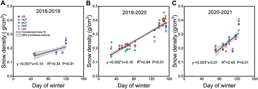
FIGURE 5. Relationship of snow density (ρ) with day of winter (DOW) for 3 years at five sites: (A) 2018–2019, (B) 2019–2020, and (C) 2020–2021. Day of winter (DOW) represents the number of days, starting from November 1 to the seasonal end of April 8. The different icons indicate different land types: OS, open site; HCF, high-intensity cutting mixed forest; MCF, moderate-intensity cutting mixed forest; NMF, natural mixed forests; LCF, low-intensity cutting mixed forest. The solid line is a fitted regression for snow density and DOW for all land types, and the shaded range indicates the 95% conference interval.
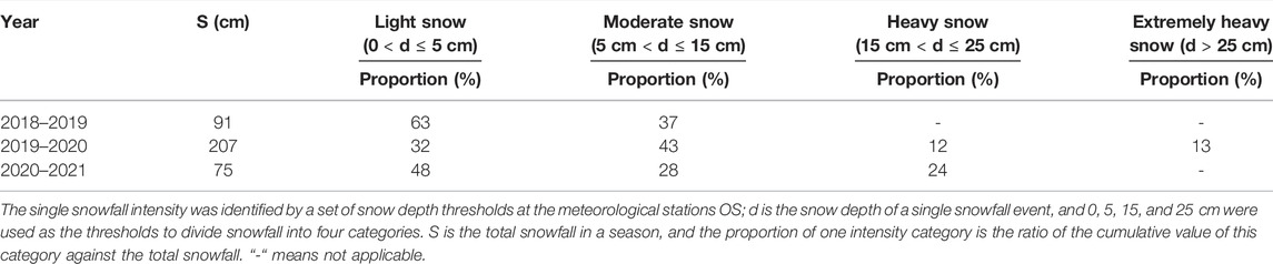
TABLE 2. Statistical characteristics of snowfall for 3 years.
The snow depth in the forest correlated to the forest canopy closure (Figure 6). The SD in the OS was greater than that in all the forests for the same SN. Moreover, the SD of the four forests in the same SN also decreased as the closure θ increased. The size order of the SD was OS > HCF > MCF > NMF > LCF (Figure 6), but the θ order was OS < HCF < MCF < NMF < LCF (Table 1), showing opposite sizes. This indicated that the forest had an obvious snow depth reduction effect. Forests with a larger θ tend to have a smaller SD.
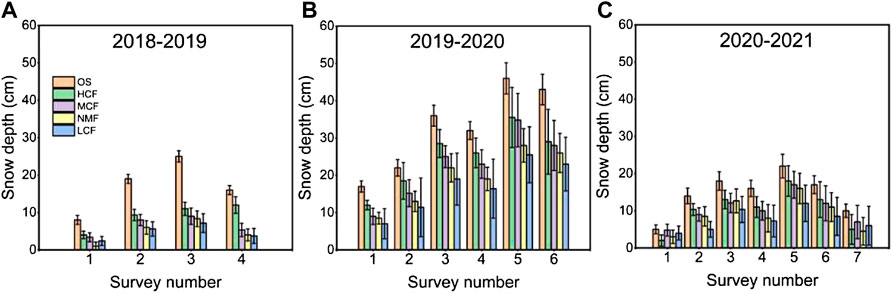
FIGURE 6. Snow depth distribution characteristics at stand level for five sites in three years, (A) 2018–2019, (B) 2019–2020, and (C) 2020–2021. The histogram is the average snow depth (SD) at the plot scale, and the error bar is the standard deviation (n = 36). Different color histograms indicate different sites: OS, open site; HCF, high-intensity cutting mixed forest; MCF, moderate-intensity cutting mixed forest; NMF, natural mixed forests; LCF, low-intensity cutting mixed forest; SD is snow depth (cm). The survey number (SN) is the serial number of the field snow survey conducted, and snow depth surveys were carried out weekly to bi-weekly.
3.3 The Relationship Between Forest Canopy Interception and Snowfall
The forest canopy interception correlated fairly with snowfall (Figure 7). The CIE of the canopy decreased as the amount of snowfall increased for an event, during 2018–2021. The CIE of the HCF, NMF, MCF, and LCF for a single snowfall event varied from 0.1 to 0.9. A single snowfall event in the study area ranged between 1.5 and 42 mm (converted to liquid water). On the whole, the CIE showed interannual variation (seeing the three sub-graphs for 3 years in Figure 7), and the fitting effectiveness of the regression curve was better in the 2019–2020 winter than in the other two winters, which was mainly because of the higher interception effect of the canopy on light snows. The proportion of the cumulative amount of light snow in the total snowfall amount was the lowest in the 2019–2020 season (Table 2). Figure 7 also shows that there was an interval difference relationship between the variation range of the interception coefficient and snowfall. The smaller the snowfall, the greater the variation range of the interception coefficient. Additionally, as snowfall increased, the variation range of the interception coefficient gradually became narrower. Furthermore, as illustrated by the fitting curves, there was a different maximum interception coefficient among different forest types. In other words, when the amount of snowfall was the same, the forest with a larger closure had a higher CIE (i.e., NMF > HCF, LCF > MCF).
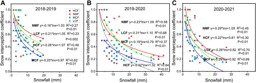
FIGURE 7. Relationship between the forest canopy interception coefficient (CIE) and snowfall for each of the three years, (A) 2018–2019, (B) 2019–2020, and (C) 2020–2021. The different icons indicate different forest types. One dot is for one snowfall event. The fitted curves are logarithmic functions of the snowfall.
3.4 The Relationship Between Canopy Closure and Snow Interception Coefficient
The snow interception coefficient is strongly related to forest canopy closure (Figure 8). The Ic and θ had a good positive correlation, and Ic increased with θ. This means that in the same year, when the θ of the forest was larger among the four forest plots, more snow was intercepted by the canopy. In the 2018–2019 winter, the Ic of the four plots varied from 0.59 to 0.9, and the forest canopy intercepted 59%–90% of the snowfall. The correlation’s slope parameter was 2.75 (R2 = 0.95). When the θ increased by 0.1, the Ic would increase by 0.27, and the corresponding snow interception increased by 27%. In the 2019–2020 winter, the Ic of the four forests varied from 0.34 to 0.73, the forest intercepted 34%–73% of the snowfall that occurred. When θ increased by 0.1, the Ic increased by 0.33 (R2 = 0.98), and the corresponding snow interception increased by 33%. In the 2020–2021 winter, the Ic of the four forests varied from 0.41 to 0.58, and the forest canopy intercepted 41%–58% of the total snowfall. For every 0.1 increase in θ, the Ic increased by 0.13 (R2 = 0.96), and the corresponding snowfall interception increased by 13%. Thus, we found that the relationship between Ic and θ was the strongest in 2019–2020, followed by in 2018–2019 and in 2020–2021. There were different linear correlations between Ic and θ in different years, indicating that the relationship had interannual variation that were largely related to changes in the annual snowfall and intensity composition of snowfall events.
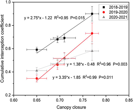
FIGURE 8. Relationship between cumulative interception coefficient (Ic) and forest canopy closure (θ). Points with different colors and shapes represent different years: the black square points represent 2018–2019, the red points represent 2019–2020, and the gray triangle points represent 2020–2021.
The interception coefficients of the four mixed forests all showed a decreasing trend as the snowfall intensity increased. This feature appeared the highest with light snow, the second highest with moderate snow, and the lowest with heavy snow and extremely heavy snow (Figure 7). As a consequence of this, when there was a higher proportion of light snow in a year, the cumulative interception was larger (Figure 8, 2018–2019), which means that when more snow was lost due to canopy interception, there was less snow understory of the canopy. From Table 2, in 2018–2019, light snow comprised 63% of the annual snowfall, and this was why the cumulative snow interception rates at the four forests in 2018–2019 were all higher than they were in the other 2 years (Figure 8).
3.5 The Relationship Between Canopy Closure and Snow Sublimation Rate
The forest canopy closure affected the snow sublimation rate (Figures 9A,C,E). There were obvious differences in the snow sublimation dynamics between the OS and the four forests. The Ss in the OS and the variation range in the 3 years were both much larger than those in the four forests over the entirety of both the Ac and Ab periods. Over the course of 3 years, the Ss in the OS varied from 0 to 4.5 mm/day, while the Ss in the four forests (HCF, MCF, NMF, and LCF) varied from 0 to 1.0 mm/day. During the different snow periods (Ac and Ab) for the same site, the Ss in the Ab period was greater than that during the Ac period (Figures 9B,D,F). Moreover, the Ss in the OS showed a much faster increase than it did in the four forests (Figure 9 left column).
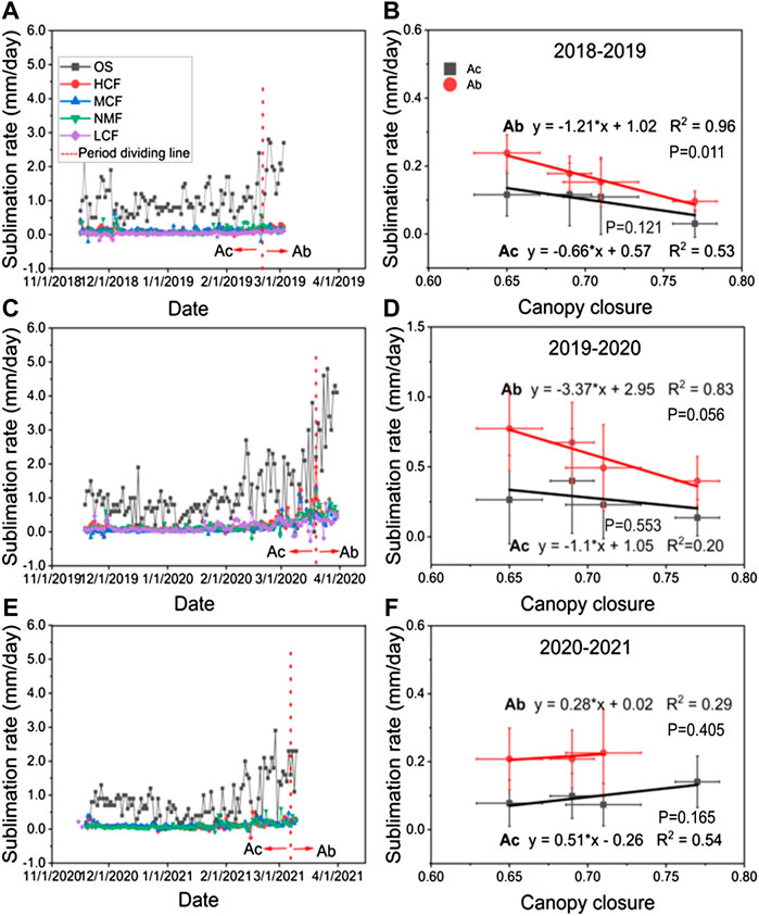
FIGURE 9. Snow sublimation rate (Ss) daily dynamics of five sites: (A) 2018–2019, (C) 2019–2020, and (E) 2020–2021; the relationship between the multi-day average snow sublimation rate (Ss-A) and forest canopy closure (θ) in the different periods: (B) 2018–2019, (D) 2019–2020, and (F) 2020–2021. Ac is the accumulation period (right column, grey point), Ab is the ablation period (right column, red point), and red dotted line (left column) is the dividing line for the Ac and Ab periods.
The forest closure affected the snow sublimation rate in both the snow accumulation and ablation periods. The snow sublimation rate (Ss) of four forests in the accumulation period was lower than that in the ablation period (Figures 9B,D,F). In 2018–2019, the Ss in the accumulation period was 0.3 ± 0.04–0.12 ± 0.14 mm/day, while it increased to 0.09 ± 0.03–0.24 ± 0.05 mm/day in the ablation period. In 2019–2020, the Ss was 0.13 ± 0.13–0.4 ± 0.37 mm/day in the snow accumulation period, while it increased to 0.39 ± 0.18–0.77 ± 0.31 mm/day in the ablation period. In 2020–2021, the Ss was 0.07 ± 0.06–0.14 ± 0.08 mm/day during the snow accumulation period and increased to 0.20 ± 0.08–0.23 ± 0.13 mm/day during the ablation period.
The effects of forest canopy closure on the snow sublimation rate showed interannual variations for both the periods. Figures 9B,D,F showed the relationship between Ss-A and θ during the different periods. The Ss-A of the four forests during the Ac and Ab periods all decreased as the θ increased for the first 2 years (2018–2019 and 2019–2020). The slope and correlation coefficient (−1.21, R2 = 0.96, 2018–2019; −3.37, R2 = 0.83, 2019–2020) were steeper and stronger during the Ab period than they were during the Ac period (−0.66, R2 = 0.53, 2018–2019; −1.1, R2 = 0.20, 2019–2020). This difference reflected how forest canopy closure had a reduction effect on Ss in 2018–2019 and 2019–2020. Additionally, the effects of forest canopy closure on snow sublimation rate during the Ab period was stronger than that in the Ac period. However, for the year 2020–2021, Ss-A and θ showed a weak positive correlation (Figure 9F), which was opposite to the correlations in the other 2 years. This indicated that forest canopy closure increased the snow sublimation rate slightly in 2020–2021.
3.6 The Relationship Between Canopy Closure and Snowmelt Rate
The snowmelt rate was also affected by forest canopy closure (Figure 10). The average Sr in the four forests was about 1.52 mm/day (2018–2019), 10.5 mm/day (2019–2020), and 2.69 mm/day (2020–2021). The large variation in the Sr among the years was related to the varying Ta and Ra. The higher they were, the higher the Sr and the faster the snowmelt. During the three Ab periods, there were different correlations between θ and Sr. The Sr was negatively correlated with θ in 2018–2019 (R2 = 0.73), and Sr decreased by 0.4 mm/day when the θ increased by 0.1. Similarly, there was a good negative correlation between Sr and θ in 2019–2020 (R2 = 0.77), and Sr decreased by 3 mm/day when the θ increased by 0.1. This suggested that elevated forest canopy closure reduced the snowmelt rate in two of the studied years. However, Sr showed a slight increase alone with the θ in 2020–2021, which indicated that the θ increased the Sr slightly during the Ab period (Sr increased by 0.79 mm/day for every 0.1 increase in θ). In summary, there was a good correlation between θ and Sr, and the relationship between them showed interannual variation.
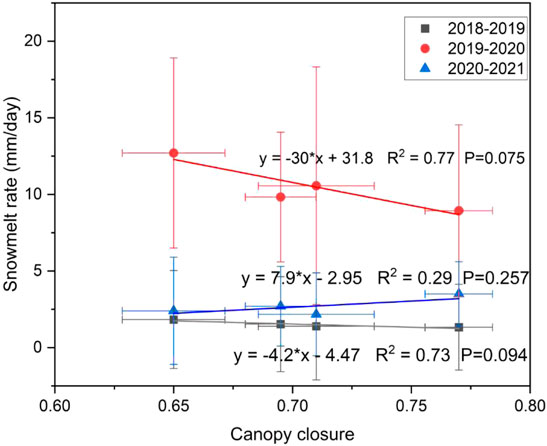
FIGURE 10. Relationship between forest canopy closure (θ) and snowmelt rate (Sr). Points of different colors and shapes represent different years. The gray square points represent 2018–2019, the red circle points represent 2019–2020, and the blue triangle points represent 2020–2021.
3.7 The Relationship Between Forest Effect on the Snow Process and Canopy Closure
Forests have a significant impact on snow processes, and with the increase of forest canopy closure, the influence of forest on snow processes also increased correspondingly (Figure 11). All four forests show a reduction in the understory surface snow water equivalent, and there is a good linear correlation between θ and the influence effect E over the 3 years. In a normal snow year (2019–2020), the E ranged from −27% to −52% among the four plots, and it decreased as θ increased across plots. Four forests showed a stronger effect on the snow in extreme low snow years (2018–2019 and 2020–2021). The mean values of the effect of the four mixed forests on understory SWE (snow water equivalent) over the 3 years ranged from −45% to −65%. Therefore, the effects of canopy closure on the forest snow processes had interannual variation. The slope of the fitted linear line (Figure 11) showed that the relationship between θ and E changed a little among different years. In 2018–2019, when θ increased by 0.1, the E of the forest on the SWE showed a relative increase of 13% (R2 = 0.98). In 2019–2020, when θ increased by 0.1, the E increased by 17% (R2 = 0.96), or in 2020–2021 it increased by 14% (R2 = 0.95). This was mainly due to the changes in snowfall characteristics in different years (Table 2). Canopy closure had a negative effect on snow processes. When θ was larger, the effect was stronger, and accordingly, there was less SWE under the forest. The higher the proportion of light snowfall annually, the stronger the influence effect of the forest on snow processes. For example, E (2019–2020) > E (2020–2021) > E (2018–2019), corresponding to the proportion of light snowfall to annual snowfall, which was 0.32 (2019–2020) < 0.48 (2020–2021) < 0.63 (2018–2019).
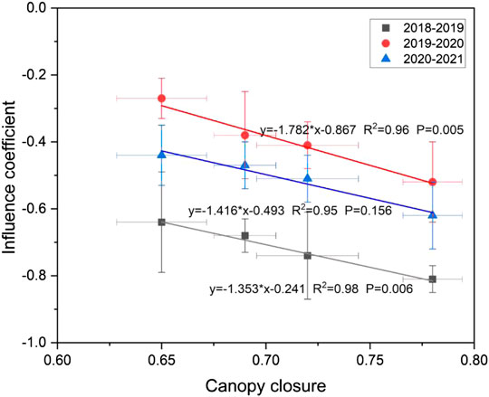
FIGURE 11. Relationship between forest influence effect (E) on snow processes and canopy closure (θ). Points of different colors and shapes represent different years.
4 Discussion
4.1 Influence Mechanisms of Forest on Snow Density and Snow Depth
Snow density and snow depth are indicators of the impacts that a forest has on snow processes. The duration date factors of snow (DOY, day of year or Julian day) have been used in snow density models: e.g., Sturm model (Lea et al., 2010) and Sexstone model (Sexstone and Fassnacht, 2014). Similar to the snow density research by Yao et al. (2018) at the Dorset Environment Science Centre site, we also found that there was a good correlation between density ρ and DOW (day of winter) during a normal snow year (R2 = 0.84, 2019–2020), indicating that the evolution of snow density can be reconstructed and characterized by DOW. However, the relationship was weak in snow-anomaly years (R2 = 0.34, 2018–2019; R2 = 0.45, 2020–2021). This indicates that snow depth (SD) should be taken into account when using the DOW to simulate snow density in less snow years. Although the snow density showed a distinguishable relationship at different sites after certain snow surveys in our study, no regular relationship was observed throughout the whole snow season. The main reason for this is that the forest canopy had a complex and persistent impact on snow density through changing a variety of comprehensive factors (such as snow depth, temperature, humidity, sublimation, and ablation), which ultimately affected the snow density under the forest canopy. A single survey event reveals only the results of the comprehensive impact of various factors on snow density in a limited period. The intensity and mechanism of different factors are changed constantly. Therefore, during the entire snow period, the snow density at various sites did not show a stable relationship with distinguishability and consistency.
The forest canopy closure affected the snow depth obviously, and the snow depth had a good relationship with the canopy closure gradient over the 3 years (Figure 6). When θ was larger, the SD was smaller. This was mainly because the greater the θ, the stronger the interception effect of the canopy on snow (Figure 8), resulting in less snow accumulating on the ground surface.
4.2 Influence Mechanism of Forest Canopy Closure on the Snow Process
Canopy closure indirectly reflects the interception area in the horizontal direction of the canopy, and it is a canopy indicator that controls the energy input and mass input to the snow surface of the understory. When the interception area increases, both the snow and energy input to the surface through the canopy are weakened. Therefore, the interception effect and influence effect decreased as θ increased (Figures 8, 11). In this study, the canopy’s interception effect on the snow was about −34% to −73%. Similar to the study by Storck et al. (2002), Roth and Nolin (2017), and Xiao et al. (2019), canopy interception was still the strongest factor affecting understory surface snow accumulation in this region. However, we found that for extreme low snow years, the canopy interception effect was stronger than in normal snow years. Additionally, the radiation transmission and wind speed under the canopy decreased as the canopy closure increased (Stähli et al., 2009), and they further changed the snow sublimation rate and snowmelt rate. All of these is the reason why the Ss in the four forests was lower than that of the open site (Figure 9), Ss and Sr both decreased as θ increased (Figures 9, 10). More importantly, at the forest stand level (40 m wide) of our study, θ showed a good correlation relationship with all the snow sub-processes (interception, sublimation, and snowmelt). Similar to previous studies on the relationship between canopy closure (or LAI) and snow processes as determined using different scales and methods by Krogh et al. (2020), Broxton et al. (2021), and Russell et al. (2021), we also found that θ was an ideal canopy index factor to explain the variations in SD, Ic, Ss, Sr, and SWE in the mixed forests of the Changbai Mountains.
Moreover, the effects of θ on Ss and Sr take place during different periods and show interannual variations. The relationship between θ and Ss or Sr appeared to be positively correlated in two of the studied years (2018–2019 and 2019–2020) but negatively correlated in the other year (2020–2021). The sublimation results in NMF forest by Li et al. (2013) showed that the sublimation rate has quadratic curves and exponential relationships with net radiation and the average temperature, respectively. Therefore, the influence of forests on snow sublimation was highly sensitive to changes in two climate factors. The multi-day Ta and Ra were −6°C and 9.95 MJ/m2 during the Ab period (2020–2021), so the energy required for snowmelt mainly came from the Ra. Because the extinction of short-wave radiation by canopy can increase the long-wave radiation of the trunk (Pomeroy et al., 2009), when the canopy has a greater θ, more energy can be absorbed by the canopy in the form of net solar radiation. This further increased the energy supply (long-wave radiation) of the snow surface and promoted the Ss and Sr of the forest snow. Therefore, Ss and Sr increased as θ increased in 2020–2021 (Figures 9, 10). The results show that the effects (positive or negative) of forest canopy closure on snow sub-processes (i.e., sublimation and snowmelt) mainly depend on the changes in different meteorological factors during the different periods.
4.3 Influence Mechanism of Snowfall on the Interaction Between Forest and Snow
The forest had a significant effect on reducing the amount of snow (Figures 6, 11). Meanwhile, there was a good negative correlation between canopy closure and the effect value (Figure 11), which is consistent with the previous research results obtained by Gelfan et al. (2004) and Varhola et al. (2010). However, the results based on the 3 years of our study showed the interannual variation in the correlation between the two. One reason was the composition of snowfall. The canopy interception coefficient was the strongest for light snow, followed by moderate snow, and was the smallest in heavy snow and extremely heavy snow (Figure 7). Accordingly, the higher the proportion of light snow, the higher effect value on the snow process. As such, forests had a stronger effect in 2018–2019 than it did during the other 2 years (Figure 11). Similarly, the proportion of light snow in 2019–2020 was the smallest (32%), and the four forests showed a smaller effect value (2019–2020) than the other 2 years. In addition, the total annual snowfall was another reason, as they had a joint effect on the snow processes. Ultimately, the impact of forests on the snow process was relatively stronger in extreme low snow years than in normal snow years. Likewise, we speculated that the intensity of the nested and interactive effects of large-scale factors (climatic conditions) and small-scale factors (forest structure) likely changed over the 3 years. This indicates that in different regions, or at different spatial scales, strong local and interannual variations may happen in the relationship between canopy closure and snow processes.
Our study serves as a case study for enriching our knowledge of forest and snow interactions. The results herein also suggest that the establishment of statistical models or physical models based on canopy structure factors in forest areas need to consider interannual effects, types of snowfall, type of forest, and scale dependences. If available, the corresponding parameters of the spatiotemporal interpolation method and remote sensing algorithm, such as the pixel decomposition algorithm by Jiang et al. (2014) and Yang et al. (2019), should be flexibly adjusted according to the relationship between SWE and forest closure in forest areas, and this may improve the accuracy of snow estimation in forest areas. Our study presents the effect of mixed forests on snow processes in the Changbai Mountain area over the course of three snow years and will compensate for the lack of snow process research in northeast China. Moreover, it may provide helpful information for forest management, snow model verification, remote sensing product development, algorithm improvement, and verification for this region in the future.
5 Conclusion
This study explored the impact of forest canopy closure on snow processes by combining in situ snow survey, eddy covariance, and water balance method to research snow processes at five sites (four forest sites and an open site). We found that forest snow processes were largely controlled by the changes in snowfall or intensity, micrometeorological conditions, and forest canopy closure. The interception of snow by the forest canopy was an important factor affecting the snow depth of understory. The forest interception effect ranged from −33% to −90%. The good correlation between forest canopy closure and the interception effect also showed interannual changes, which were mainly related to different snowfall events. Changes in forest closure altered the snow sublimation and snowmelt processes, and canopy closure showed a good correlation with the snow sublimation rate and snowmelt rate. Compared to the open site, the four mixed forests affected the SWE of understory by −27% to −81% and strongly reduced the SWE over the 3 years. Canopy closure can explain well the impact of mixed forest structure changes on the snow processes in the Changbai Mountain area. We also found that there were interannual variations in the impact effects caused by forest closure on the snow processes, suggesting that dynamic effects need to be considered when comparing snow models in forest area or when conducting the snow mapping tasks. More importantly, changes in snowfall caused by future winter warming may further complicate the impact of forests on snow processes in this region.
Data Availability Statement
The original contributions presented in the study are included in the article/supplementary material; further inquiries can be directed to the corresponding author.
Author Contributions
YG and LS contributed to conception and design of the study. YG and RC organized the database and performed the statistical analysis. YG wrote the first draft of the manuscript. LS, AW, FY, JW, DG, and HY revised the manuscript and provided for revision. All authors contributed to manuscript revision and read and approved the submitted version.
Funding
This research was supported by the National Natural Science Foundation of China (Grant Nos. 31971728, 32171873, 41975150, and 31870625).
Conflict of Interest
The authors declare that the research was conducted in the absence of any commercial or financial relationships that could be construed as a potential conflict of interest.
Publisher’s Note
All claims expressed in this article are solely those of the authors and do not necessarily represent those of their affiliated organizations, or those of the publisher, the editors and the reviewers. Any product that may be evaluated in this article, or claim that may be made by its manufacturer, is not guaranteed or endorsed by the publisher.
References
Bebi, P., Kulakowski, D., and Rixen, C. (2009). Snow Avalanche Disturbances in Forest Ecosystems-State of Research and Implications for Management. For. Ecol. Manag. 257 (9), 1883–1892. doi:10.1016/j.foreco.2009.01.050
Broxton, P. D., Harpold, A. A., Biederman, J. A., Troch, P. A., Molotch, N. P., and Brooks, P. D. (2015). Quantifying the Effects of Vegetation Structure on Snow Accumulation and Ablation in Mixed‐conifer Forests. Ecohydrol. 8 (6), 1073–1094. doi:10.1002/eco.1565
Broxton, P. D., Moeser, C. D., and Harpold, A. (2021). Accounting for Fine‐Scale Forest Structure is Necessary to Model Snowpack Mass and Energy Budgets in Montane Forests. Water Resour. Res. 57, e2021WR029716. doi:10.1029/2021WR029716
Burles, K., and Boon, S. (2011). Snowmelt Energy Balance in a Burned Forest Plot, Crowsnest Pass, Alberta, Canada. Hydrol. Process. 25, 3012–3029. doi:10.1002/hyp.8067
Casteller, A., Häfelfinger, T., Cortés Donoso, E., Podvin, K., Kulakowski, D., and Bebi, P. (2018). Assessing the interaction between mountain forests and snow avalanches at Nevados de Chillan, Chile and its implications for ecosystem-based disaster risk reduction. Nat. Hazards Earth Syst. Sci. 18 (4), 1173–1186. doi:10.5194/nhess-18-1173-2018
Chang, J., Wang, G.-x., Gao, Y.-h., and Wang, Y.-b. (2014). The Influence of Seasonal Snow on Soil Thermal and Water Dynamics under Different Vegetation Covers in a Permafrost Region. J. Mt. Sci. 11 (3), 727–745. doi:10.1007/s11629-013-2893-0
Charuchittipan, D., Babel, W., Mauder, M., Leps, J.-P., and Foken, T. (2014). Extension of the Averaging Time in Eddy-Covariance Measurements and its Effect on the Energy Balance Closure. Boundary-Layer Meteorol. 152 (3), 303–327. doi:10.1007/s10546-014-9922-6
De Roo, F., Zhang, S., Huq, S., and Mauder, M. (2018). A Semi-empirical Model of the Energy Balance Closure in the Surface Layer. PLoS One 13 (12), e0209022. doi:10.1371/journal.pone.0209022
Dong, C., and Menzel, L. (2017). Snow Process Monitoring in Montane Forests with Time-Lapse Photography. Hydrol. Process. 31 (16), 2872–2886. doi:10.1002/hyp.11229
Dong, C. (2018). Remote Sensing, Hydrological Modeling and In Situ Observations in Snow Cover Research: A Review. J. Hydrol. 561, 573–583. doi:10.1016/j.jhydrol.2018.04.027
Ellis, C. R., Pomeroy, J. W., Brown, T., and MacDonald, J. (2010). Simulation of Snow Accumulation and Melt in Needleleaf Forest Environments. Hydrol. Earth Syst. Sci. 14 (6), 925–940. doi:10.5194/hess-14-925-2010
Frazer, G. W., Canham, C. D., and Lertzman, K. P. (1999). Gap Light Analyzer (GLA): Imaging Software to Extract Canopy Structure and Gap Light Transmission Indices from True-Colour Fisheye Photographs, Users Manual and Program Documentation. Burnaby, Millbrook, NY: Simon Fraser University, Institute of Ecosystem Studies.
Frei, A., Tedesco, M., Lee, S., Foster, J., Hall, D. K., Kelly, R., et al. (2012). A Review of Global Satellite-Derived Snow Products. Adv. Space Res. 50 (8), 1007–1029. doi:10.1016/j.asr.2011.12.021
Garvelmann, J., Pohl, S., and Weiler, M. (2012). Applying a Time-Lapse Camera Network to Observe Snow Processes in Mountainous Catchments. doi:10.5194/hessd-9-10687-2012
Gelfan, A. N., Pomeroy, J. W., and Kuchment, L. S. (2004). Modeling Forest Cover Influences on Snow Accumulation, Sublimation, and Melt. J. Hydrometeorol. 5 (5), 785–803. doi:10.1175/1525-7541(2004)005<0785:mfcios>2.0.co;2
Guan, D.-X., Wu, J.-B., Zhao, X.-S., Han, S.-J., Yu, G.-R., Sun, X.-M., et al. (2006). CO2 Fluxes over an Old, Temperate Mixed Forest in Northeastern China. Agric. For. Meteorol. 137 (3-4), 138–149. doi:10.1016/j.agrformet.2006.02.003
Hao, J., Mind'je, R., Feng, T., and Li, L. (2021). Performance of Snow Density Measurement Systems in Snow Stratigraphies. Hydrol. Res. 52 (4), 834–846. doi:10.2166/nh.2021.133
Harpold, A. A., Guo, Q., Molotch, N., Brooks, P. D., Bales, R., Fernandez-Diaz, J. C., et al. (2014). LiDAR-derived Snowpack Data Sets from Mixed Conifer Forests across the Western United States. Water Resour. Res. 50 (3), 2749–2755. doi:10.1002/2013wr013935
Henderson, G. R., Peings, Y., Furtado, J. C., and Kushner, P. J. (2018). Snow-atmosphere Coupling in the Northern Hemisphere. Nat. Clim. Change 8 (11), 954–963. doi:10.1038/s41558-018-0295-6
Hojatimalekshah, A., Uhlmann, Z., Glenn, N. F., Hiemstra, C. A., Tennant, C. J., Graham, J. D., et al. (2021). Tree Canopy and Snow Depth Relationships at Fine Scales with Terrestrial Laser Scanning. Cryosphere 15 (5), 2187–2209. doi:10.5194/tc-15-2187-2021
Jacobs, J. M., Hunsaker, A. G., Sullivan, F. B., Palace, M., Burakowski, E. A., Herrick, C., et al. (2021). Snow Depth Mapping with Unpiloted Aerial System Lidar Observations: a Case Study in Durham, New Hampshire, United States. Cryosphere 15 (3), 1485–1500. doi:10.5194/tc-15-1485-2021
Jiang, L., Wang, P., Zhang, L., Yang, H., and Yang, J. (2014). Improvement of Snow Depth Retrieval for FY3B-MWRI in China. Sci. China Earth Sci. 57 (6), 1278–1292. doi:10.1007/s11430-013-4798-8
Krinner, G., Derksen, C., Essery, R., Flanner, M., Hagemann, S., Clark, M., et al. (2018). ESM-SnowMIP: Assessing Snow Models and Quantifying Snow-Related Climate Feedbacks. Geosci. Model Dev. 11 (12), 5027–5049. doi:10.5194/gmd-11-5027-2018
Krogh, S. A., Broxton, P. D., Manley, P. N., and Harpold, A. A. (2020). Using Process Based Snow Modeling and Lidar to Predict the Effects of Forest Thinning on the Northern Sierra Nevada Snowpack. Front. For. Glob. Change 3, 21. doi:10.3389/ffgc.2020.00021
Lea, J., Jonas, T., Derksen, C., Liston, G.E., Taras, B., and Sturm, M. (2010). Estimating Snow Water Equivalent Using Snow Depth Data and Climate Classes. J. Hydrometeorol. 11 (6), 1380–1394. doi:10.1175/2010jhm1202.1
Lendzioch, T., Langhammer, J., and Jenicek, M. (2019). Estimating Snow Depth and Leaf Area Index Based on UAV Digital Photogrammetry. Sensors 19 (5), 1027. doi:10.3390/s19051027
Li, H. D., Guan, D. X., Wang, A. Z., Wu, J. B., Jin, C. J., and ShiI, T. T. (2013). Characteristics of Evaporation over Broadleaved Korean Pine Forest in Changbai Mountains, Northeast China during Snow Cover Period in Winter. Ying Yong Sheng Tai Xue Bao 24 (4), 1039–1046. doi:10.13287/j.1001-9332.2013.0278
Li, H., Wang, A., Guan, D., Jin, C., Wu, J., Yuan, F., et al. (2016). Empirical Model Development for Ground Snow Sublimation beneath a Temperate Mixed Forest in Changbai Mountain. J. Hydrol. Eng. 21 (11), 04016040. doi:10.1061/(asce)he.1943-5584.0001415
López-Moreno, J. I., and Nogués-Bravo, D. (2006). Interpolating Local Snow Depth Data: an Evaluation of Methods. Hydrol. Process. 20 (10), 2217–2232. doi:10.1002/hyp.6199
Lopez-Moreno, J. I., and Stahli, M. (2008). Statistical Analysis of the Snow Cover Variability in a Subalpine Watershed: Assessing the Role of Topography and Forest, Interactions. J. Hydrol. 348 (3-4), 379–394. doi:10.1016/j.jhydrol.2007.10.018
Lundquist, J. D., Dickerson-Lange, S. E., Lutz, J. A., and Cristea, N. C. (2013). Lower Forest Density Enhances Snow Retention in Regions with Warmer Winters: A Global Framework Developed from Plot-Scale Observations and Modeling. Water Resour. Res. 49 (10), 6356–6370. doi:10.1002/wrcr.20504
Lyu, Z., and Zhuang, Q. (2018). Quantifying the Effects of Snowpack on Soil Thermal and Carbon Dynamics of the Arctic Terrestrial Ecosystems. J. Geophys. Res. Biogeosci. 123 (4), 1197–1212. doi:10.1002/2017jg003864
Mauder, M., Cuntz, M., Drüe, C., Graf, A., Rebmann, C., Schmid, H. P., et al. (2013). A Strategy for Quality and Uncertainty Assessment of Long-Term Eddy-Covariance Measurements. Agric. For. Meteorol. 169, 122–135. doi:10.1016/j.agrformet.2012.09.006
Maurer, G. E., and Bowling, D. R. (2014). Seasonal Snowpack Characteristics Influence Soil Temperature and Water Content at Multiple Scales in Interior Western U.S. Mountain Ecosystems. Water Resour. Res. 50 (6), 5216–5234. doi:10.1002/2013wr014452
Maxwell, J. D., Call, A., and St. Clair, S. B. (2019). Wildfire and Topography Impacts on Snow Accumulation and Retention in Montane Forests. For. Ecol. Manag. 432, 256–263. doi:10.1016/j.foreco.2018.09.021
Montesi, J., Elder, K., Schmidt, R. A., and Davis, R. E. (2004). Sublimation of Intercepted Snow within a Subalpine Forest Canopy at Two Elevations. J. Hydrometeorol. 5 (5), 763–773. doi:10.1175/1525-7541(2004)005<0763:soiswa>2.0.co;2
Musselman, K. N., Molotch, N. P., Margulis, S. A., Kirchner, P. B., and Bales, R. C. (2012). Influence of Canopy Structure and Direct Beam Solar Irradiance on Snowmelt Rates in a Mixed Conifer Forest. Agric. For. Meteorol. 161, 46–56. doi:10.1016/j.agrformet.2012.03.011
Napoly, A., Boone, A., and Welfringer, T. (2020). ISBA-MEB (SURFEX v8.1): Model Snow Evaluation for Local-Scale Forest Sites. Geosci. Model Dev. 13 (12), 6523–6545. doi:10.5194/gmd-13-6523-2020
O'Gorman, P. A. (2014). Contrasting Responses of Mean and Extreme Snowfall to Climate Change. Nature 512 (7515), 416–418. doi:10.1038/nature13625
Parajka, J., Haas, P., Kirnbauer, R., Jansa, J., and Blöschl, G. (2012). Potential of Time-Lapse Photography of Snow for Hydrological Purposes at the Small Catchment Scale. Hydrol. Process. 26 (22), 3327–3337. doi:10.1002/hyp.8389
Parajuli, A., Nadeau, D. F., Anctil, F., Parent, A.-C., Bouchard, B., Girard, M., et al. (2020). Exploring the Spatiotemporal Variability of the Snow Water Equivalent in a Small Boreal Forest Catchment through Observation and Modelling. Hydrol. Process. 34 (11), 2628–2644. doi:10.1002/hyp.13756
Perrot, D., Molotch, N. P., Musselman, K. N., and Pugh, E. T. (2014). Modelling the Effects of the Mountain Pine Beetle on Snowmelt in a Subalpine Forest. Ecohydrol. 7 (2), 226–241. doi:10.1002/eco.1329
Pomeroy, J. W., Gray, D. M., Hedstrom, N. R., and Janowicz, J. R. (2002). Prediction of Seasonal Snow Accumulation in Cold Climate Forests. Hydrol. Process. 16 (18), 3543–3558. doi:10.1002/hyp.1228
Pomeroy, J. W., Gray, D. M., Brown, T., Hedstrom, N. R., Quinton, W. L., Granger, R. J., et al. (2007). The Cold Regions Hydrological Model: a Platform for Basing Process Representation and Model Structure on Physical Evidence. Hydrol. Process. 21 (19), 2650–2667. doi:10.1002/hyp.6787
Pomeroy, J. W., Marks, D., Link, T., Ellis, C., Hardy, J., Rowlands, A., et al. (2009). The Impact of Coniferous Forest Temperature on Incoming Longwave Radiation to Melting Snow. Hydrol. Process. 23 (17), 2513–2525. doi:10.1002/hyp.7325
Pomeroy, J., Fang, X., and Ellis, C. (2012). Sensitivity of Snowmelt Hydrology in Marmot Creek, Alberta, to Forest Cover Disturbance. Hydrol. Process. 26 (12), 1891–1904. doi:10.1002/hyp.9248
Pugh, E., and Gordon, E. (2013). A Conceptual Model of Water Yield Effects from Beetle-Induced Tree Death in Snow-Dominated Lodgepole Pine Forests. Hydrol. Process. 27 (14), 2048–2060. doi:10.1002/hyp.9312
Reichstein, M., Falge, E., Baldocchi, D., Papale, D., Aubinet, M., Berbigier, P., et al. (2005). On the Separation of Net Ecosystem Exchange into Assimilation and Ecosystem Respiration: Review and Improved Algorithm. Glob. Change Biol. 11 (9), 1424–1439. doi:10.1111/j.1365-2486.2005.001002.x
Revuelto, J., López-Moreno, J.-I., Azorin-Molina, C., Alonso-González, E., and Sanmiguel-Vallelado, A. (2016). Small-Scale Effect of Pine Stand Pruning on Snowpack Distribution in the Pyrenees Observed with a Terrestrial Laser Scanner. Forests 7 (8), 166. doi:10.3390/f7080166
Roth, T. R., and Nolin, A. W. (2017). Forest Impacts on Snow Accumulation and Ablation across an Elevation Gradient in a Temperate Montane Environment. Hydrol. Earth Syst. Sci. 21 (11), 5427–5442. doi:10.5194/hess-21-5427-2017
Russell, M., Eitel, J. U. H., Link, T. E., and Silva, C. A. (2021). Important Airborne Lidar Metrics of Canopy Structure for Estimating Snow Interception. Remote Sens. 13 (20), 4188. doi:10.3390/rs13204188
Rutter, N., Essery, R., Pomeroy, J., Altimir, N., Andreadis, K., Baker, I., et al. (2009). Evaluation of Forest Snow Processes Models (SnowMIP2). J. Geophys. Res. 114, D06111. doi:10.1029/2008JD011063
Schelker, J., Kuglerová, L., Eklöf, K., Bishop, K., and Laudon, H. (2013). Hydrological Effects of Clear-Cutting in a Boreal Forest - Snowpack Dynamics, Snowmelt and Streamflow Responses. J. Hydrol. 484, 105–114. doi:10.1016/j.jhydrol.2013.01.015
Schwartz, A. J., McGowan, H., and Callow, N. (2020). Impact of Fire on Montane Snowpack Energy Balance in Snow Gum Forest Stands. Agric. For. Meteorol. 294, 108164. doi:10.1016/j.agrformet.2020.108164
Sexstone, G. A., and Fassnacht, S. R. (2014). What Drives Basin Scale Spatial Variability of Snowpack Properties in Northern Colorado? Cryosphere 8 (2), 329–344. doi:10.5194/tc-8-329-2014
Sexstone, G. A., Clow, D. W., Fassnacht, S. R., Liston, G. E., Hiemstra, C. A., Knowles, J. F., et al. (2018). Snow Sublimation in Mountain Environments and its Sensitivity to Forest Disturbance and Climate Warming. Water Resour. Res. 54 (2), 1191–1211. doi:10.1002/2017wr021172
Stähli, M., Jonas, T., and Gustafsson, D. (2009). The Role of Snow Interception in Winter-Time Radiation Processes of a Coniferous Sub-alpine Forest. Hydrol. Process. 23 (17), 2498–2512. doi:10.1002/hyp.7180
Steele, C., Dialesandro, J., James, D., Elias, E., Rango, A., and Bleiweiss, M. (2017). Evaluating MODIS Snow Products for Modelling Snowmelt Runoff: Case Study of the Rio Grande Headwaters. Int. J. Appl. Earth Observ, Geoinf. 63, 234–243. doi:10.1016/j.jag.2017.08.007
Storck, P., Lettenmaier, D. P., and Bolton, S. M. (2002). Measurement of Snow Interception and Canopy Effects on Snow Accumulation and Melt in a Mountainous Maritime Climate, Oregon, United States. Water Resour. Res. 38 (11), 5–1516. doi:10.1029/2002wr001281
Varhola, A., and Coops, N. C. (2013). Estimation of Watershed-Level Distributed Forest Structure Metrics Relevant to Hydrologic Modeling Using LiDAR and Landsat. J. Hydrol. 487, 70–86. doi:10.1016/j.jhydrol.2013.02.032
Varhola, A., Coops, N. C., Weiler, M., and Moore, R. D. (2010). Forest Canopy Effects on Snow Accumulation and Ablation: An Integrative Review of Empirical Results. J. Hydrol. 392 (3-4), 219–233. doi:10.1016/j.jhydrol.2010.08.009
Veatch, W., Brooks, P. D., Gustafson, J. R., and Molotch, N. P. (2009). 'Quantifying the Effects of Forest Canopy Cover on Net Snow Accumulation at a Continental, Mid-latitude Site'. Ecohydrol. 2 (2), 115–128. doi:10.1002/eco.45
Watson, F. G. R., Anderson, T. N., Newman, W. B., Alexander, S. E., and Garrott, R. A. (2006). Optimal Sampling Schemes for Estimating Mean Snow Water Equivalents in Stratified Heterogeneous Landscapes. J. Hydrol. 328 (3-4), 432–452. doi:10.1016/j.jhydrol.2005.12.032
Webb, E. K., Pearman, G. I., and Leuning, R. (1980). Correction of Flux Measurements for Density Effects Due to Heat and Water Vapour Transfer. Q.J R. Metall. Soc. 106, 85–100. doi:10.1002/qj.49710644707
Wilczak, J. M., Oncley, S. P., and Stage, S. A. (2001). Sonic Anemometer Tilt Correction Algorithms. Boundary-Layer Meteorol. 99 (1), 127–150. doi:10.1023/A:1018966204465
Woods, S. W., Ahl, R., Sappington, J., and McCaughey, W. (2006). Snow Accumulation in Thinned Lodgepole Pine Stands, Montana, USA. For. Ecol. Manag. 235 (1-3), 202–211. doi:10.1016/j.foreco.2006.08.013
Wu, J., Guan, D., Yuan, F., Yang, H., Wang, A., and Jin, C. (2012). Evolution of Atmospheric Carbon Dioxide Concentration at Different Temporal Scales Recorded in a Tall Forest. Atmos. Environ. 61, 9–14. doi:10.1016/j.atmosenv.2012.07.013
Xiao, Y., Li, X., Zhao, S., and Song, G. (2019). Characteristics and Simulation of Snow Interception by the Canopy of Primary Spruce‐fir Korean Pine Forests in the Xiaoxing'an Mountains of China. Ecol. Evol. 9 (10), 5694–5707. doi:10.1002/ece3.5152
Yang, J., Jiang, L., Dai, L., Pan, J., Wu, S., and Wang, G. (2019). The Consistency of SSM/I vs. SSMIS and the Influence on Snow Cover Detection and Snow Depth Estimation over China. Remote Sens. 11 (16), 1879. doi:10.3390/rs11161879
Yao, H., McConnell, C., James, A., and Fu, C. (2012). Comparing and Modifying Eight Empirical Models of Snowmelt Using Data from Harp Experimental Station in Central Ontario. Br. J. Environ. Clim. Change 2, 259–277. doi:10.9734/bjecc/2012/2249
Yao, H., Field, T., McConnell, C., Beaton, A., and James, A. L. (2018). Comparison of Five Snow Water Equivalent Estimation Methods across Categories. Hydrol. Process. 32 (12), 1894–1908. doi:10.1002/hyp.13129
Keywords: forest canopy closure, forest snow, interception, sublimation, snowmelt
Citation: Gao Y, Shen L, Cai R, Wang A, Yuan F, Wu J, Guan D and Yao H (2022) Impact of Forest Canopy Closure on Snow Processes in the Changbai Mountains, Northeast China. Front. Environ. Sci. 10:929309. doi: 10.3389/fenvs.2022.929309
Received: 26 April 2022; Accepted: 20 May 2022;
Published: 01 July 2022.
Edited by:
Bo Huang, Norwegian University of Science and Technology, NorwayReviewed by:
Weibin Li, Lanzhou University, ChinaMeng Yang, Nanjing University of Information Science and Technology, China
Copyright © 2022 Gao, Shen, Cai, Wang, Yuan, Wu, Guan and Yao. This is an open-access article distributed under the terms of the Creative Commons Attribution License (CC BY). The use, distribution or reproduction in other forums is permitted, provided the original author(s) and the copyright owner(s) are credited and that the original publication in this journal is cited, in accordance with accepted academic practice. No use, distribution or reproduction is permitted which does not comply with these terms.
*Correspondence: Lidu Shen, c2hlbmxpZHVAaWFlLmFjLmNu