Spatial downscaling of surface ozone concentration calculation from remotely sensed data based on mutual information

Accurate near surface ozone concentration calculation with high spatial resolution data is very important to solve the problem of serious ozone pollution and health impact assessment. However, the existing remotely sensed ozone products cannot meet the requirements of high spatial resolution monitoring. In this study, surface O₃ concentration (at 30 km spatial resolution) was extracted from the daily TROPOMI O₃ profile products. Meanwhile, this study improved the downscaling algorithm based on the mutual information and applied it to the mapping of surface O₃ concentration in China. Combined with the surface O₃ concentration data (with 5 km spatial resolution) obtained by using the Light Gradient Boosting Machine (LightGBM) algorithm and AOD data (at 1 km resolution) from MODIS, the downscaling of TROPOMI ground O₃ concentration data from 30 km to 1 km has been achieved in this study. The downscaled ground O₃ concentration data were subsequently validated using an independent ground O₃ concentration dataset. The main conclusion of this study is that the mutual information entropy between the bottom layer data of the TROPOMI ozone profile (at 30 km resolution), LightGBM surface O₃ concentration data (at 5 km resolution), and MCD19A2 AOD data (at 1 km resolution) can accurately reduce the spatial resolution of ozone concentration in the ground layer. The downscaling procedure not only resulted in increase of the spatial resolution over the whole area but also significant improvements in precision with coefficient of determination (R²) increased from 0.733 to 0.823, mean biased error decreased from 7.905 μg/m³ to 3.887 μg/m³, and root-mean-square error decreased from 14.395 μg/m³ to 8.920 μg/m³ for ground O₃ concentration.

Introduction

With the continuous development and changes of economy and society, air pollution, especially surface-level ozone (O₃) pollution, has been paid more and more attention by the states and people. Different from upper-layer ozone, which is the Earth’s protective umbrella, surface ozone is a polluting gas that can cause photochemical smog, causing many problems to climate change (Skeie et al., 2011; Shindell et al., 2012; Stevenson et al., 2013), ecosystem (Victoria et al., 2009; Ainsworth et al., 2012; Yue and Unger, 2014), and human health (Ebi and McGregor, 2008; Lim et al., 2012; Chen et al., 2017), when the higher ozone concentration is located near the ground surface (0–3 km height). If people are exposed to ozone pollution for a long time, they will suffer from nausea, respiratory inflammation, and other diseases, and even damage lung function or death. Several large population studies in the United States have confirmed that ozone pollution and population mortality are dose-dependent, especially for children, elderly, and patients with some basic diseases (Chen et al., 2017).

In recent years, morbidity and mortality rates related to ozone have increased in many countries (Aaron et al., 2017), and it has become the main culprit of atmospheric environmental pollution in many cities in summer and autumn, second only to particulate matter with a diameter < 2.5 μm (PM_2.5). At present, the most accurate means of surface-level ozone monitoring is measurement by using ground receiving instruments and generate real-time data. In order to monitor air pollution, China has successively established more than 1500 trace gas monitoring stations (Adam-Poupart et al., 2014; Madaniyazi et al., 2016; Sun et al., 2018) in various provinces and cities to measure the hourly local ground O₃ concentration since 2013, which provides strong support for the study of ground O₃. However, the ground detection stations only detect the air quality in the study area in point distribution, with poor spatial resolution and extremely uneven spatial distribution. At the same time, ozone is highly reactive, so their ground-level values are influenced by the deposition process, which in turn depends on the dominant land use. This also adds spatial heterogeneity everywhere. Due to the spatial heterogeneity of ground-level O₃ and the uneven distribution of ground detection stations, traditional spatial interpolation methods cannot obtain high-precision O₃ concentration values and their spatial distribution characteristics.

A space-based remote sensing method such as geostationary remote sensing (Lee et al., 2019) provides the potential to assess long-term trends in atmospheric O₃ concentrations over wide areas to fill the in situ monitoring gaps. However, discriminating O₃ at the surface level from the whole-atmosphere O₃ columns is challenging because only about 10% of the O₃ is within the lower troposphere (Hayashida et al., 2018). Based on the current development level of satellite remote sensing technology, there is no sensor that can directly obtain the ground layer O₃ data (as shown in Table 1), but the spatial resolution of the ground O₃ concentration is too rough to use.

TABLE 1

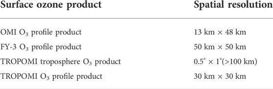
TABLE 1. Surface ozone product and its spatial resolution. OMI, ozone monitoring instrument; FY-3, Fengyun-3 satellite; and TROPOMI, TROPOspheric Monitoring Instrument.

Therefore, downscaling the existing ground O₃ concentration map to obtain higher resolution round O₃ concentration data is of great practical significance to environmental management, disease prevention, research, and other industries. There are three downscaling methods in remote sensing (Atkinson, 2013): 1) assumptions or prior knowledge about the character of the target spatial variation coupled with spatial optimization, 2) spatial prediction through interpolation, and 3) direct information on the relation between spatial resolutions in the form of a downscaling (such as regression) model. Among them, methods 1) and 2) are less effective in improving the spatial resolution or increasing the information contained. At present, there are many studies on obtaining ground ozone by using method 3.

Among many studies that use downscaling models to estimate the O₃ concentration in the high-resolution ground-level, machine learning or deep learning models are mostly used, such as the geographically weighted regression (GWR) model (Zhang et al., 2020), space-time extremely randomized trees (STET) algorithm (Wei et al., 2021), multivariate adaptive regression splines (MARS) model (Gauthier-Manuel et al., 2022), gradient boosting regression tree (GBRT) algorithm (Gauthier-Manuel et al., 2022), and spatiotemporally embedded deep residual neural network (STE-ResNet) model (Li and Cheng, 2021). The basic principle of these downscaling methods is the same. First, relevant data such as meteorological data, satellite images, reanalysis data, emission data, or others are spatiotemporally matched and input into the machine learning model or the deep learning model as independent variables. Then the O₃ measurement of the ground station is taken as the dependent variable, and the mapping relationship between the independent variable and the dependent variable is obtained by using the powerful computing ability of the learning model. Finally, the ground-level O₃ concentration in the high-resolution is estimated by using this mapping relationship. These algorithms are different in the selection of independent variables, selection of models, input nodes of variables, verification methods of estimation results, and so on.

The mechanism opacity and relatively poor scalability of the learning model also make the relevant research questioned to a certain extent. However, this cannot hide the high accuracy and resolution of the calculation results of such methods, and many of them have also achieved novel and effective results in spatiotemporal information. Li and Cheng (2021) proposed to embed time and space into the deep learning model as classification variables so that the model estimation has higher accuracy in time and space (Li and Cheng, 2021). Sun et al. (2021) used the spatiotemporal indices as mandatory inputs to the spatiotemporal statistical model to reproduce the spatiotemporal autocorrelation of their observations (Sun et al., 2021).

Therefore, this study tried to combine the high-quality results of the machine learning model with the non-learning downscaling model (mutual information algorithm) to improve its interpretability and reliability while maintaining its high-resolution and high-accuracy characteristics. In this study, a downscale estimation method of ground O₃ concentration over China based on the mutual information (MI) entropy model is improved, and the downscaling of ground ozone concentration from 30 km to 1 km was realized.

Data

The ground ozone concentration of the TROPOspheric Monitoring Instrument

The TROPOspheric Monitoring Instrument (TOPOMI), mounted on the Sentinel-5 Predictor (Sentinel-5P) satellite, is an atmospheric monitoring spectrometer with the most advanced technical performance and the highest spatial resolution so far. Sentinel-5P was launched on 13 October 2017 and flew in the polar orbit and the solar synchronous orbit. The time for the satellite to cross the equator is about 13:30 local time. TROPOMI O₃ profile data were officially released in November 2021. The classic ozone profile retrieval algorithm (optimal estimation method, OE) was used to retrieve the ozone profile, with an original spatial resolution of 30 km × 30 km (ESA, 2021a). In order to ensure the accuracy of the data, this study eliminated bad values of the ozone profile provided by TROPOMI according to the following three aspects (ESA, 2021b):

1) If the data quality value ($qa\_value$) is too low, it is not recommended (ESA, 2021b).

$\begin{array}{c}qa\_value\le 0.5.\end{array}(1)$

2) Inspection of the data shows that for some of the retrievals unphysical solutions are found, which pass the $qa\_value$ filtering guidelines provided in Eq. 1. Therefore, it is recommended to disregard a pixel that matches the following criteria (ESA, 2021b).

$\begin{array}{c}{\sum }_{i=0}^{i=32}\left|n\left(i\right)-n_{ap}\left(i\right)\right|>1.66\times {10}^{-5}mole\bullet m^{-3},\end{array}(2)$

where $i$ is index for the altitude or pressure level, $n\left(i\right)$ is the ozone concentration in $mole\bullet m^{-3}$, and $n_{ap}\left(i\right)$ is the a priori ozone concentration.

3) The fitting quality of some ground pixels (especially in polar regions) is low. These data can be filtered by removing pixels for which the $cost\_function$ data field exceeds 200 (ESA, 2021b).

$\begin{array}{c}cost\_function>200\end{array}(3)$

The obtained ozone profile is divided into 33 layers from the ground to 1Pa (about 80 km) at the vertical height of the atmosphere. The typical ozone profile is shown in Figure 1. In addition, the ozone concentration of each layer of the ozone profile product provided by TROPOMI is in $mole\bullet m^{-3}$, which can be converted into micrograms per cubic meter ($\mu g\bullet m^{-3}$) through the following formula, where $M$ is the molar mass of ozone and its value is 48 g/mol.

$\begin{array}{c}O3\mathit{PR}\left(mol\bullet m^{-3}\right)\times M\left(g\bullet {mol}^{-1}\right)\times {10}^6=O3\mathit{PR}\left(\mu g\bullet m^{-3}\right).\end{array}(4)$

FIGURE 1

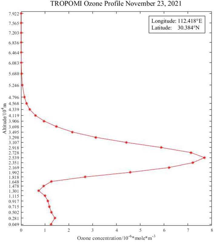
FIGURE 1. Tropomi ozone profile (November 23, 2021).

As shown in Figure 1, the bottom layer data of TROPOMI ozone profile are the inversion data of ozone profile concentration about 500 m away from the surface. This study separated this part of data and converted the unit into micrograms per cubic meter ($\mu g\bullet m^{-3}$), consistent with ground observation stations. Then this part of data was evaluated by the observation data at the corresponding positions.

Figure 2 shows the evaluation results of the measured O₃ concentration of the station about the original ground O₃ data extracted from the profile data. The determination coefficient (R²) is 0.672, the root-mean-square error (RMSE) is 17.973 μg/m³, and the average deviation error (MBE) is 7.836 μg/m³, which indicates that the bottom layer data of the TROPOMI ozone profile have good correlation with the measured O₃ concentration at the station, and there is little difference. The normalized root-mean-square error (nRMSE) is 29.789%, which is also within a reasonable range, indicating that the bottom layer data of the TROPOMI ozone profile can be used to characterize the ground O₃ concentration to a certain extent.

FIGURE 2

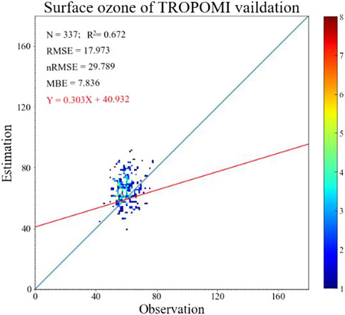
FIGURE 2. Validation result of the TROPOMI surface-level ozone concentration map in 30 km. N means total matched points, R² is the correlation coefficient, RMSE is the root-mean-square error, nRMSE is the normalized root-mean-square error, and MBE represents mean biased error. The solid blue line is the 1:1 line. The solid red line is the fitting line of observation and surface ozone of TROPOMI, and the equation marked in red is the fitting formula, where X represents surface ozone observation and Y represents surface ozone of TROPOMI. The color bars in (a)-(l) indicate the number of samples in the 1.5 μg/m³ square.

The ground ozone concentration of the Light Gradient Boosting Machine algorithm

The surface O₃ concentration dataset covering China can be used to assist the downscaling of surface O₃ concentration. Based on the analysis of the source and the sink of ground ozone, the Light Gradient Boosting Machine (LightGBM) algorithm (Ke et al., 2017) was used to fuse various satellite-based variables (from TROPOMI), meteorological variables based on numerical models (from the European Centre for Medium-Range Weather Forecasts, ECWMF), and land variables (from National Aeronautics and Space Administration, NASA) to estimate the surface O₃ concentration (The details of the aforementioned variables are shown in Table 2). That model was developed to estimate surface ozone mass concentrations by selecting relevant data corresponding to each component of the source and the sink as independent variables and in situ surface O₃ concentration as dependent variables (Kang et al., 2021). The time of LightGBM algorithm estimation in this study is 13:30 local time daily, and the spatial resolution is 0.05° × 0.05° (about 5 km × 5 km). In that case, LightGBM model parameters were set as follows: boosting_type = “gbdt,” objective = “regression,” learning_rate = 0.07, metric = “rmse,” max_depth = 9, min_child_weight = 0.01, min_child_samples = 20, reg_alpha = 0.03, reg_lambda = 0.05, n_estimators = 167, task = “train,” feature_fraction = 0.98, bagging_fraction = 0.92, num_leaves = 200, and bagging_freq = 5. The LightGBM model is verified by the 10-fold cross-validation random method. Figure 3 shows the verification results. The estimated mass concentration of surface ozone is in good agreement with the measured value at ground stations, with a high correlation coefficient (R² = 0.959) and a relatively low RMSE (9.483 μg/m³).

TABLE 2

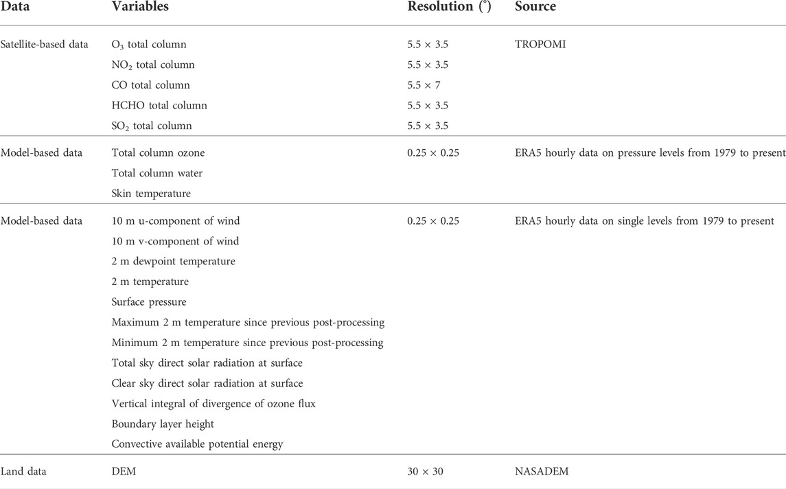
TABLE 2. Independent variables of the LightGBM model.

FIGURE 3

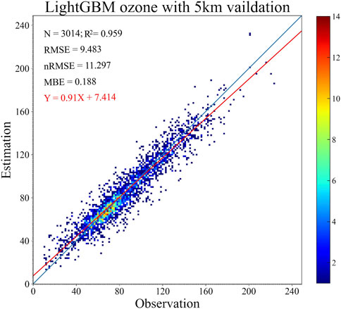
FIGURE 3. Estimated value and ground station cross-validation results of surface-level O₃.

Using the aforementioned model, the surface O₃ concentration dataset with 5 km resolution covering China was obtained. The dataset, as part of the development of MI model in this study, was used to improve the accuracy of downscaling results.

The aerosol optical depth product of moderate resolution imaging spectrometer

Many studies have pointed out that the complex physical and chemical characteristics of aerosols would affect the formation and loss of O₃ in the ground layer (Shao et al., 2017). Aerosol particles can change the atmospheric heterogeneous reaction process, which can affect the formation of O₃ (Li et al., 2014; Lou et al., 2014). In addition, the absorption and scattering of radiation by external aerosol particles can affect the photolysis process of O₃ precursor, which also affects the formation of O₃ (Li et al., 2014; Lou et al., 2014). In the Earth’s atmosphere, there is a certain correlation between O₃ and aerosol optical depth (AOD), as one of the most important parameters of aerosol. Many studies have found that when the solar radiation is strong, the formation of near surface O₃ is also quite sensitive to the change of AOD (Ran et al., 2009; Pozzoli et al., 2011). At the same time, some studies (such as Kang et al. (2021)) have used AOD as input data when estimating surface ozone concentration.

Moderate resolution imaging spectrometer (MODIS) has 36 bands. It is a large space remote sensing instrument developed by National Aeronautics and Space Administration (NASA) to understand the changes of global climate and the impact of human activities on climate. It can provide surface parameters such as surface temperature and the vegetation index with different temporal and spatial resolutions (Han et al., 2018; Cao et al., 2019). In this study, the aerosol optical depth product (MCD19A2) was selected for the downscaling of O₃ concentration map in the ground. MCD19A2 is the shortname for the multi-angle implementation of atmospheric correction (MAIAC) algorithm–based level-2 gridded (L2G) aerosol optical thickness over land surfaces product (Lyapustin et al., 2018). This product is obtain using Terra and Aqua MODIS input with daily 1 km resolution, which is available from NASA’s website (https://ladsweb.modaps.eosdis.nasa.gov/) for free. In this study, the product with high spatial resolution and close relationship with ground O₃, as a part of the development of the MI model, was used to reduce the spatial scale of ground O₃ concentration data.

The ground-based measurements

The measured O₃ concentration data (2021, Figure 4) of stations used in this study are from the national air quality data provided by the National Real-Time Release Platform for Urban Air Quality of the China National Environmental Monitoring Station, with a total of 1925 stations. In addition, in order to ensure the accuracy of the data, this study eliminated the invalid values (null) and abnormal values (greater than 1000 and less than 0) caused by instrument calibration problems. Because of the limited temporal resolution of TROPOMI, the present study targeted once a day (i.e., 13:30 local time). The observation data used in this study were the average values at 13:00 and 14:00, which is consistent with TROPOMI and LightGBM data.

FIGURE 4

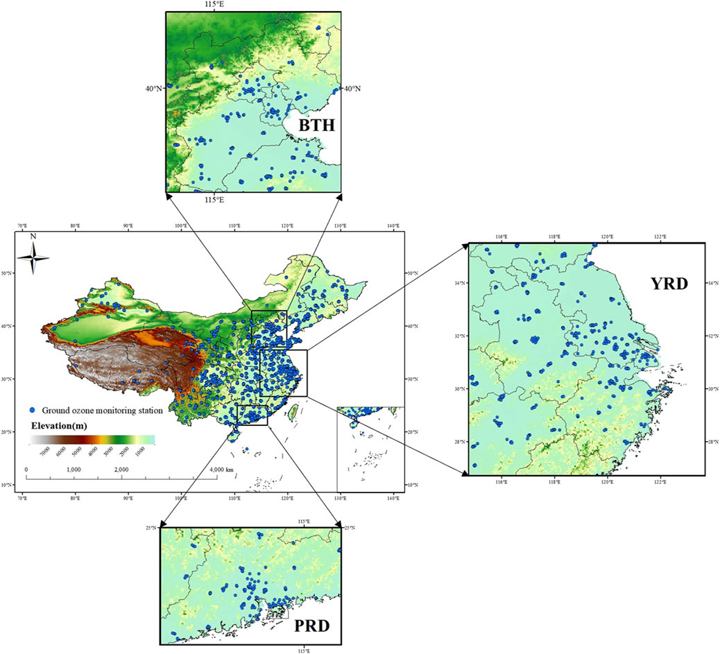
FIGURE 4. Spatial distributions of ground O₃ monitoring stations (blue dots) in 2021 across China, where the background is surface elevation (m). The uppermost, lowermost, and rightmost panels show the three regions of interest in this study: the Beijing–Tianjin–Hebei (BTH) region, Pearl River Delta (PRD), and Yangtze River Delta (YRD).

At the same time, the ground-based measured O₃ concentration dataset was randomly divided into a calibration subset (90%) and a test subset (10%). The calibration subset was used as a dependent variable in the LightGBM model to calibrate the model and generate a 5 km LightGBM surface ozone dataset, whereas the test subset was used as an independent ground O₃ concentration dataset to validate and evaluate the accuracy of input data (30 km TROPOMI surface O₃ concentration data, 5 km LightGBM surface O₃ concentration data, and 1 km MCD19A2 AOD data) and MI method results.

Methodology

The overall procedure of the downscaling surface O₃ concentrations, shown in Figure 5, consists of two parts: 1) model development and 2) model evaluation. First, the original ground O₃ concentration data with relatively low resolution was extracted through the TROPOMI O₃ profile product. Second, the MI downscaling model was developed to obtain the 1 km TROPOMI ground O₃ concentration by inputting the 30 km TROPOMI surface O₃ data, 5 km LightGBM O₃ data, and 1 km MODIS AOD data into it. Then the MI downscaling model was validated with the hourly ground monitoring station dataset followed by the description of error.

FIGURE 5

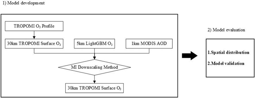
FIGURE 5. Process flow diagram for downscaling transformation of surface O₃ concentration guided by mutual information entropy.

Model development

Mutual information (MI) is an important concept in information theory, which can represent a measure of the relative entropy between two sets and can be described as a measure of information redundancy. Generally speaking, MI can represent the amount of information about variable X in the random vector Y. From this definition, it can be easily shown that the MI of two images is at its maximum when these two images are identical (Johnson et al., 2001). In MI computing, if $X$ and $Y$ are two images, then the joint probability distribution is $p\left(x,y\right)$ of $X$ and $Y$, when $p\left(x\right)$ and $p\left(y\right)$ are defined as the marginal probability distributions. The entropy of $X$ and $H\left(X\right)$ is then defined as follows (Shannon, 1948):

$\begin{array}{c}H\left(X\right)=-{\displaystyle \sum }_{x}p\left(x\right)logp\left(x\right),\end{array}(5)$

$\begin{array}{c}H\left(Y\right)=-{\displaystyle \sum }_{y}p\left(y\right)logp\left(y\right).\end{array}(6)$

The joint entropy of $X$, $Y$, and $H\left(X,Y\right)$ is as follows (Li et al., 2012):

$\begin{array}{c}H\left(X,Y\right)=-{\displaystyle \sum }_x{\displaystyle \sum }_{y}p\left(x,y\right)logp\left(x,y\right).\end{array}(7)$

So that the mutual information of $X$, $Y$, and $MI\left(X,Y\right)$ is as follows (Li et al., 2012):

$\begin{array}{c}MI\left(X,Y\right)=H\left(X\right)+H\left(Y\right)-H\left(X,Y\right)=-{\displaystyle \sum }_{xy}p\left(x,y\right)\mathit{log}\frac{p\left(x,y\right)}{p\left(x\right)p\left(y\right)}.\end{array}(8)$

Also, in the actual calculation, the joint probability distribution $p\left(X,Y\right)$ is typically replaced by a joint histogram $\mathcal{h}\left(X,Y\right)$ (Li et al., 2012):

$\begin{array}{c}p\left(x,y\right)=\frac{h\left(x,y\right)}{{\displaystyle \sum }_{x,y}h\left(x,y\right)},\end{array}(9)$

$\begin{array}{c}p\left(x\right)={\displaystyle \sum }_{y}p\left(x,y\right),p\left(y\right)={\displaystyle \sum }_{x}p\left(x,y\right).\end{array}(10)$

The downscaling method based on MI was first proposed by Li et al. (2012). In the study of Li et al., the MI between the MODIS image and the CCD upscaled image was maximized by adjusting the coefficients, so as to obtain the weights and coefficients required for downscaling transformation (Li et al., 2012). Finally, they realized the downscaling of MODIS image from 500 m to 100 m by using these weights and coefficients.

This study comprehensively coordinated all the spatial scales and strictly matched and aligned each input data based on the spatial scale of the original ground O₃ concentration data (as shown in Figure 6). In order to realize the downscaling of TROPOMI ground O₃ concentration data from 30 km to 1 km, the assumptions of this study are as follows (Li et al., 2012):

1) The downscaled image should contain the information and physical meaning of both the two original images;

2) The MI between the downscaled images and the LightGBM surface O₃ concentration image should be maximized;

3) The downscaling should be reversible that means if we upscale the downscaled image back, it should be as the same as the original;

4) The physical meaning of the downscaled image should be remained.

FIGURE 6

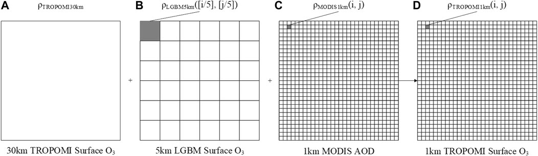
FIGURE 6. Downscaling of 30 km TROPOMI surface O₃ pixel to 1 km pixels.

In Figure 6, 5 km LightGBM surface O₃ image and 1 km MODIS AOD image are shown as 6 × 6 and 30 × 30 pixel matrixes, respectively, which corresponds to a 30 km TROPOMI surface O₃ pixel on the left. On the far right, there are the downscaled 1 km TROPOMI surface O₃ pixels in the box. Each pixel value in it should contain the information of 30 km TROPOMI surface O₃ pixel, 5 km LightGBM surface O₃ pixel, and 1 km MODIS AOD pixels and keep them within the effective range. In addition, the MI value between 1 km TROPOMI surface O₃ image and 5 km LightGBM surface O₃ image should be maximized. According to these assumptions, the pixel downscaling transformation formula in this study should be as follows:

${\rho }_{TROPOMI1km}\left(i,j\right)=k_1{\rho }_{TROPOMI30km}+k_2{\rho }_{LGBM5km}\left(\left[i/5\right],\left[j/5\right]\right)$

$\begin{array}{c}+k_3{\rho }_{MOSID1km}\left(i,j\right)+k_4\end{array}(11)$

where ${\rho }_{TROPOMI30km}$ is the value of a 30 km TROPOMI surface O₃ pixel; ${\rho }_{MOSID1km}$ and ${\rho }_{TROPOMI1km}$ are the value of 1 km MODIS AOD pixel and 1 km TROPOMI surface O₃ pixel located at $\left(i,j\right)$ in the box, respectively; ${\rho }_{LGBM5km}$ is the value of 5 km LightGBM surface O₃ pixel located at $\left(\left[i/5\right],\left[j/5\right]\right)$ in the box. In the formula, $k_1$, $k_2$, $k_3$, and $k_4$ are coefficients where $k_1$, $k_2$, and $k_3$ are the weights of 30 km TROPOMI surface O₃, 5 km LightGBM surface O₃, and 1 km MODIS AOD images, respectively, and $k_4$ is an adjustment coefficient that is used to fit the assumptions 3) and 4).

During parameter estimation, we first set the initial weights $k_1$, $k_2$, and $k_3$ according to the characteristics of different inputs (such as uncertainty), and then we calculated Eq. 11. When the downscaled image data violates assumptions 3) or 4), we would use the adjustment coefficient $k_4$ to make it meet assumptions 1), 2), 3), and 4) at the same time. Then we calculated the MI between the downscaled image and the 5 km LightGBM surface O₃ image and judged whether this MI value was the current maximum value. Finally, we continuously iterated the above process until getting $k_1$, $k_2$, $k_3$, and $k_4$ that can satisfy assumptions 1), 2), 3), and 4) simultaneously and has the largest MI. In this way, we can make the downscaling transformation results to have sufficient physical coincidence with the original data and supplement the details of the high-resolution image.

Model evaluation

In order to evaluate the performance of the proposed models, the test subset of ground-based O₃ observation data was used in this study to validate the accuracy of the model. The accuracy evaluation index—coefficient of determination (R²), root-mean-square error (RMSE), normalized root-mean-square error (nRMSE), and mean biased error (MBE) —were used.

$\begin{array}{c}{R}^2=\frac{{\sum }_{i=1}^n\left|\left(x_i-\overline{x}\right)\left(y_i-\overline{y}\right)\right|}{\sqrt{{\sum }_{i=1}^n{\left(x_i-\overline{x}\right)}^2{\sum }_{i=1}^n{\left(y_i-\overline{y}\right)}^2}},\end{array}(12)$

$\begin{array}{c}RMSE=\sqrt{\frac{{\sum }_{i=1}^n{\left(x_i-y_i\right)}^2}{n}},\end{array}(13)$

$\begin{array}{c}nRMSE=\frac{100\times \sqrt{\frac{{\sum }_{i=1}^n{\left(x_i-y_i\right)}^2}{n}}}{\overline{y}},\end{array}(14)$

$\begin{array}{c}MBE=\frac{{\sum }_{i=1}^n\left(x_i-y_i\right)}{n},\end{array}(15)$

where $x_i$ and $y_i$ are the result and observed data, respectively; $\overline{x}$ and $\overline{y}$ are the mean of the result and observed data, respectively, when $n$ is the number of the observations. The value of R² indicates the degree of the correlation between the result data and the observed data. $R^2=1$ indicates complete correlation, and $R^2=0$ indicates that the observation data is completely irrelevant to the result data. RMSE representing the deviation between the observed data and the result data. The nRMSE is calculated by dividing the RMSE by the mean observed data, which was used to prevent judgment errors due to the size of units and numbers (Bouman and van Laar, 2006). MBE measures the average bias between observed and result data, using the same scale as the data being measured, $\mu g\bullet m^{-3}$.

Results

Spatial distribution

The Figures 7A–C are 30 km TROPOMI surface O₃ concentration data, 5 km LightGBM surface O₃ concentration data, and 1 km MCD19A2 AOD data as model input data, respectively, and the corresponding time of the data used in this study is daily 13:30 local time. Figure 7D is the downscaling result of 30 km TROPOMI surface O₃ concentration data based on the MI method, which contains the information from Figures 7A–C. However, Figure 7D added many fine texture features and spatial details, compared with Figure 7A. Figure 7E is the round-based O₃ observation data, which was used to validate the aforementioned data.

FIGURE 7

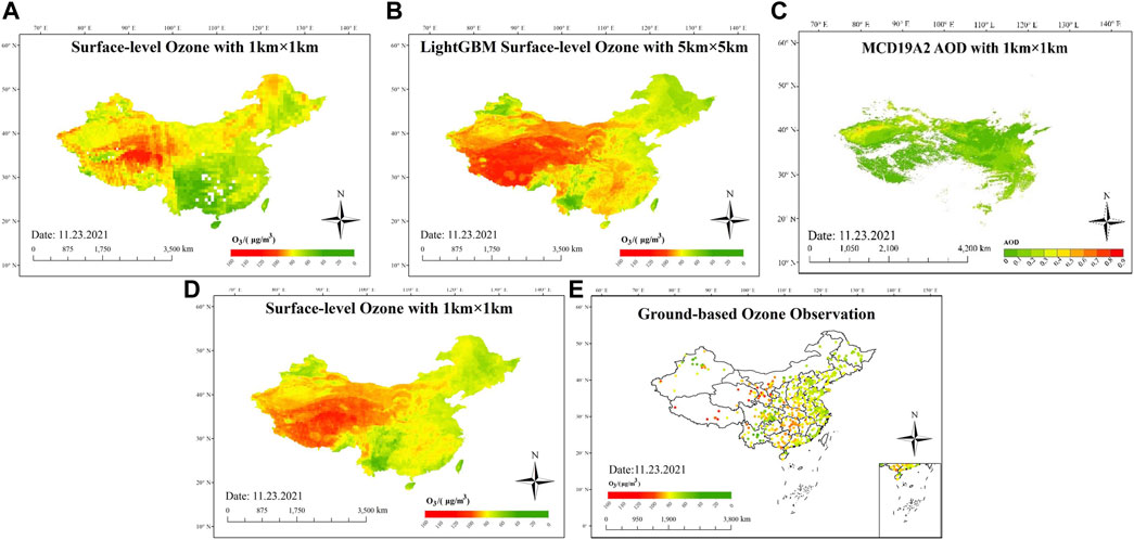
FIGURE 7. Downscaled result based on the MI method. (A) 30 km TROPOMI surface O₃ concentration image, (B) 5 km LightGBM surface O₃ concentration image, (C) 1 km MCD19A2 AOD image,(D) 1 km TROPOMI surface O₃ concentration image based on MI method, and (E) ground-based O₃ observation image.

In Figure 7A, there is a small amount of missing data, which is the result of eliminating the bad value of the bottom data of the original TROPOMI O₃ profile product. The missing amount is small and has little impact on the final downscaling result. Through comparison, it can be found that there is a very obvious spatial correlation between 30 km TROPOMI surface O₃ data image and 5 km LightGBM surface O₃ data image: The highest values of surface O₃ concentration appear in the Qinghai Tibet Plateau, and the low value surrounds the high value step by step with the Qinghai Tibet Plateau as the center.

The 1 km MCD19A2 AOD data image (Figure 6C) also shows a certain correlation compared with the two ground O₃ concentration maps (a) and (b). For example, the values in the middle part are relatively low and the values on both sides are relatively high. In addition, due to the limitation of inversion algorithm and the influence of cloud interference, there is a certain lack of effective value in Figure 6C (Levy et al., 2013). In order to avoid this situation in the downscaling result image, this study adopted the cubic convolution interpolation method to realize the downscaling of spatial resolution from 5km to 1 km at the corresponding position where AOD data is missing, which based on the calculation results of MI method. This method is based on the calculation results of MI model with 30 km TROPOMI surface O₃ concentration data and 5 km LightGBM surface O₃ data as inputs.

From the perspective of spatial distribution, Figure 6D has great spatial correlation with Figures 6A,B have great spatial correlation, which shows that this downscaling result does not lose its spatial geographical features while improving the accuracy and spatial resolution. However, there are many fine texture features and spatial details in Figure 6D which are not available in Figure 6A, enabling it to further indicate more detailed ground ozone concentration characteristics. These data can provide a reasonable and reliable basis for pollution supervision and the prevention and control of epidemic diseases caused by high O₃ concentration.

Figure 7E shows the ground-based O₃ observation data, covering almost the whole of China. However, due to geographical and economic constraints, the distribution of these stations is very uneven. Although the distribution of stations is very sparse in western and northern China, its value can also correspond to the surface ozone concentration at the corresponding position in Figure 7D. Meanwhile, the observed values of ground stations in other areas of China are very related to the surface ozone concentration at the corresponding position in Figure 7D. It can be seen that the improved MI downscaling method in this study can not only reduce the data scale of surface ozone concentration but also ensure that its accuracy is not lost.

Figure 8 shows the spatial distribution of the three regions of interest in this study. Among them, the Beijing–Tianjin–Hebei (BTH) region, the Yangtze River Delta (YRD) region and Pearl River Delta (PRD) are relatively developed regions in China, which have been affected by O₃ pollution for a long time and have attracted more attention. Figures 8A–C show the initial ground O₃ concentration in the YRD region, BTH region, and PRD region, respectively. Figures 8D–F show the performance of 1 km ozone concentration values after downscaling by MI model in the YRD region, BTH region, and PRD region, respectively, and the corresponding ground observation values are shown on them. Through comparison, it is found that in these key urban areas, MI models can significantly improve their information richness. However, the specific spatial distribution is still different. Among them, the coincidence degree of spatial distribution of images in the BTH region before and after downscaling is the best. Although, the images of the YRD region and the PRD region before and after downscaling can also ensure that the overall concentration change trend is consistent, they are not completely consistent in detail. This is the performance of the increase in the amount of information and therefore the increase in accuracy. In addition, the results show that the measured O3 concentrations at these sites are in close agreement with those estimated by the MI model.

FIGURE 8

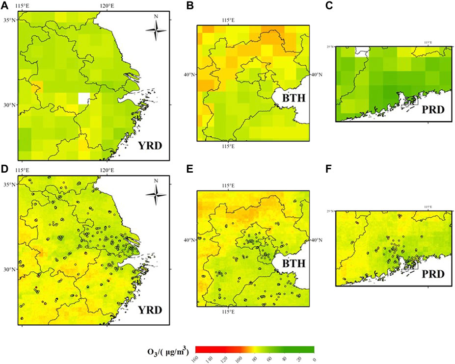
FIGURE 8. Downscaling results based on the MI method in YRD, BTH, and PRD. (A) and (D) are the 30 km TROPOMI surface O₃ concentration image and the 1 km TROPOMI surface O₃ concentration image based on the MI method in BTH, respectively. (B) and (E) are the 30 km image and 1 km image in YRD, respectively. (C) and (F) are the 30 km image and 1 km image in PRD, respectively.

Model validation

In this study, the ground observation O₃ concentration dataset was used to verify the effectiveness of the MI downscaling method in the mapping of ground O₃ concentration data. We extracted the original low resolution TRTOPOMI surface O₃ concentration data and downscaling result data of the station location and calculated the validation index. The verification result (23 November 2021) is shown in Figure 9. The downscaled 1 km TROPOPMI surface O₃ concentration is good agreement with the measured value at ground stations, with a high determination coefficient (R² = 0.877) and a relatively low RMSE (7.385 μg/m³), nRMSE (11.471%), and MBE (2.893 μg/m³). Compared with the index of original data (R² = 0.668, RMSE = 14.533 μg/m³, nRMSE = 24.365%, and MBE = 5.761 μg/m³), it can be concluded that the downscaling procedure significantly increased the determination coefficient R² and reduced RMSE, nRMSE, and MBE. The downscaled ground O₃ concentration images have higher accuracy than the 30 km TROPOMI surface O₃ concentration images, and its spatial resolution has been greatly improved, which shows that the improved MI downscaling method in this study has a good application prospect.

FIGURE 9

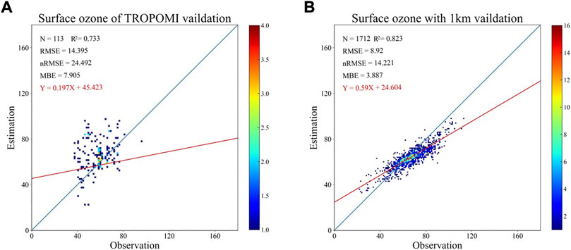
FIGURE 9. Validation of surface O₃ concentration downscaling results (23 November 2021). (A) Validation of original 30 km TROPOPMI surface O₃ concentration data and (B) validation of downscaled 1 km TROPOPMI surface O₃ concentration data.

We further tested the model performance in interest regions in China. This model is most applicable in the Yangtze River Delta (YRD, Figure 10B) region with coefficient of determination R² values of 0.925. The model performance is slightly poorer (e.g., R² = 0.786 and R² = 0.888) in the Beijing–Tianjin–Hebei (BTH, Figure 10A) region and the Pearl River Delta (PRD, Figure 10C). Overall, there are certain uncertainties in the model, and also certain differences in the robustness of the model in different regions (e.g., RMSE = 3.962–8.253 μg/m³, nRMSE = 6.253–13.603 μg/m3, and MBE = −0.519–6.998), which is also the direction we will continue to work on next.

FIGURE 10

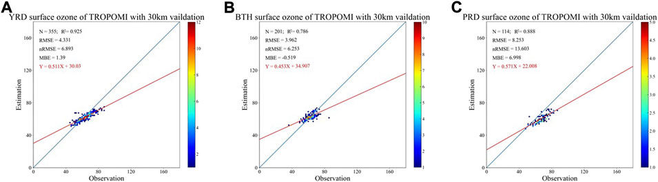
FIGURE 10. Validation of surface O₃ concentration downscaling results (23 November 2021). (A) Yangtze River Delta (YRD), (B) Beijing-Tianjin-Hebei (BTH) region, (C) Pearl River Delta (PRD) region.

Conclusion

This study improved a downscaling method based on mutual information, using TROPOMI O₃ profile product (at 30 km resolution), LightGBM surface O₃ concentration data (at 5 km resolution), and MCD19A2 AOD data (at 1 km resolution). The TROPOMI surface O₃ concentration data (at 1 km resolution) was obtained, and the downscaling results were validated using the observation data of the ground monitoring station. The improved downscaling method based on MI significantly resulted in very significant improvements in the spatial resolution and accuracy of TROPOMI surface O₃ concentration data. In the subsequent studies, the analysis of annual and seasonal variations in surface O₃ and some test of significance will be carried out.

Data availability statement

The original contributions presented in the study are included in the article/supplementary material; further inquiries can be directed to the corresponding author.

Author contributions

XW is responsible for the idea proposal, literature inquiry, data download, data experiment, analysis of experimental results, chart making, main content writing, and integration; YX is responsible for guiding and checking the content of the article, revising the manuscript, communication, and academic interpretation of the manuscript; CJ provided the original verification code of ground ozone concentration map based on ground station data and assisted in the production of Figure 3; YS helped to download and process MCD19A2 data; NL provided the processing code of MCD19A2 data.

Funding

This work was supported in part by the National Natural Science Foundation of China (NSFC) under Grant No. 41871260. The TROPOMI data and ERA5 hourly data were obtained from the ESA Copernicus Open Access Hub and the European Centre for Medium-Range Weather Forecasts (ECWMF). The MCD19A2 AOD data were obtained from EARTHDATA Open Access for Open Science. The ground measurement data for validation are from National Real-Time Release Platform for Urban Air Quality in China.

Acknowledgments

The authors thank all the principal investigators and their staff for providing the data and products used in this investigation.

Conflict of interest

The authors declare that the research was conducted in the absence of any commercial or financial relationships that could be construed as a potential conflict of interest.

Publisher’s note

All claims expressed in this article are solely those of the authors and do not necessarily represent those of their affiliated organizations, or those of the publisher, the editors, and the reviewers. Any product that may be evaluated in this article, or claim that may be made by its manufacturer, is not guaranteed or endorsed by the publisher.

References

Aaron, J. C., Michael, B., Richard, B., H, R. A., Joseph, F., Kara, E., et al. (2017). Estimates and 25-year trends of the global burden of disease attributable to ambient air pollution: An analysis of data from the global burden of diseases study 2015. Lancet 389 (10082), 1907–1918. doi:10.1016/s0140-6736(17)30505-6

PubMed Abstract | CrossRef Full Text | Google Scholar

Adam-Poupart, A., Brand, A., Fournier, M., Jerrett, M., and Smargiassi, A. (2014). Spatiotemporal modeling of ozone levels in quebec (Canada): A comparison of kriging, land-use regression (LUR), and combined bayesian maximum entropy-LUR approaches. Environ. health Perspect. 122 (9), 970–976. doi:10.1289/ehp.1306566

PubMed Abstract | CrossRef Full Text | Google Scholar

Ainsworth, E. A., Yendrek, C. R., Sitch, S., Collins, W. J., and Emberson, L. D. (2012). The effects of tropospheric ozone on net primary productivity and implications for climate change. Annu. Rev. Plant Biol. 63 (1), 637–661. doi:10.1146/annurev-arplant-042110-103829

PubMed Abstract | CrossRef Full Text | Google Scholar

Atkinson, P. M. (2013). Downscaling in remote sensing. Int. J. Appl. Earth Observation Geoinformation 22, 106–114. doi:10.1016/j.jag.2012.04.012

CrossRef Full Text | Google Scholar

Bouman, B. A. M., and van Laar, H. H. (2006). Description and evaluation of the rice growth model ORYZA2000 under nitrogen-limited conditions. Agric. Syst. 87 (3), 249–273. doi:10.1016/j.agsy.2004.09.011

CrossRef Full Text | Google Scholar

Cao, Y., Yuan, Y., Zheng, X., and Zhou, S. (2019). Study on cloud characteristics in huaibei area based on MODIS data. J. remote Sens. 23 (02), 349–358.

Google Scholar

Chen, L., Zhao, C., Guan, M., and Song, J. (2017). Current situation of air ozone pollution and its impact on population health in China. Environ. Occup. Med. 34 (11), 1025–1030.

Google Scholar

Ebi, K. L., and McGregor, G. (2008). Climate change, tropospheric ozone and particulate matter, and health impacts. Environ. health Perspect. 116 (11), 1449–1455. doi:10.1289/ehp.11463

PubMed Abstract | CrossRef Full Text | Google Scholar

ESA (2021b). S5P mission performance Centre ozone profile. [ L2__O3__PR] Readme, URL: https://sentinel.esa.int/documents/247904/3541451/Sentinel-5P-Ozone-profile-Product-Readme-File.pdf.

Google Scholar

ESA (2021a). Sentinel-5P-TROPOMI-ATBD-Ozone-Profile. URL: https://sentinel.esa.int/documents/247904/2476257/Sentinel-5P-TROPOMI-ATBD-Ozone-Profile.pdf.

Google Scholar

Gauthier-Manuel, H., Mauny, F., Boilleaut, M., Ristori, M., Pujol, S., Vasbien, F., et al. (2022). Improvement of downscaled ozone concentrations from the transnational scale to the kilometric scale: Need, interest and new insights. Environ. Res. 210, 112947. doi:10.1016/j.envres.2022.112947

PubMed Abstract | CrossRef Full Text | Google Scholar

Han, H., Bai, J., Zhang, B., and Ma, G. (2018). Temporal and spatial variation characteristics of vegetation phenology in Shaanxi Province Based on MODIS time series. Remote Sens. land Resour. 30 (04), 125–131. doi:10.6046/gtzyyg.2018.04.19

CrossRef Full Text | Google Scholar

Hayashida, S., Kajino, M., Deushi, M., Sekiyama, T. T., and Liu, X. (2018). Seasonality of the lower tropospheric ozone over China observed by the Ozone Monitoring Instrument. Atmos. Environ. 184, 244–253. doi:10.1016/j.atmosenv.2018.04.014

CrossRef Full Text | Google Scholar

Johnson, K., ColeRhodes, A., Zavorin, I., and Le Moigne, J. (2001). “Mutual information as a similarity measure for remote sensing image registration,” in Morgan state univ. (United States);Univ. Of Maryland/College Park and NASA goddard space flight ctr. (United States);NASA goddard space flight ctr. (United States), 438, 351–361.

Google Scholar

Kang, Y., Choi, H., Im, J., Park, S., Shin, M., Song, C., et al. (2021). Estimation of surface-level NO2 and O3 concentrations using TROPOMI data and machine learning over East Asia. Environ. Pollut. 288, 117711. doi:10.1016/j.envpol.2021.117711

PubMed Abstract | CrossRef Full Text | Google Scholar

Ke, G., Meng, Q., Finley, T., Wang, T., Chen, W., Ma, W., et al. (2017). “LightGBM: A highly efficient gradient boosting decision tree,” in 31st conference on neural information processing systems (Long Beach, CA: NIPS), 3149–3157.

Google Scholar

Lee, S. J., Ahn, M. H., and Ha, S. (2019). Total column ozone retrieval from the infrared measurements of a geostationary imager. IEEE Trans. Geosci. Remote Sens. 57 (8), 5642–5650. doi:10.1109/tgrs.2019.2901173

CrossRef Full Text | Google Scholar

Levy, R. C., Mattoo, S., Munchak, L. A., Remer, L. A., Sayer, A. M., Hsu, N. C., et al. (2013). The Collection 6 MODIS aerosol products over land and ocean. Atmos. Meas. Tech. 6 (1), 2989–3034. doi:10.5194/amt-6-2989-2013

CrossRef Full Text | Google Scholar

Li, T., and Cheng, X. (2021). Estimating daily full-coverage surface ozone concentration using satellite observations and a spatiotemporally embedded deep learning approach. Int. J. Appl. Earth Observation Geoinformation 101, 102356. doi:10.1016/j.jag.2021.102356

CrossRef Full Text | Google Scholar

Li, Y., Xue, Y., He, X., and Jie, G. (2012). High-resolution aerosol remote sensing retrieval over urban areas by synergeticuse of HJ-1 CCD and MODIS data. Atmos. Environ. 46, 173–180. doi:10.1016/j.atmosenv.2011.10.002

CrossRef Full Text | Google Scholar

Li, J., Han, Z., and Zhang, R. (2014). Influence of aerosol hygroscopic growth parameterization on aerosol optical depth and direct radiative forcing over East Asia. Atmos. Res. 140-141, 14–27. doi:10.1016/j.atmosres.2014.01.013

CrossRef Full Text | Google Scholar

Lim, S. S., Vos, T., Flaxman, A. D., Danaei, G., Shibuya, K., Adair-Rohani, H., et al. (2012). A comparative risk assessment of burden of disease and injury attributable to 67 risk factors and risk factor clusters in 21 regions, 1990–2010: A systematic analysis for the global burden of disease study 2010. Lancet 380 (9859), 2224–2260. doi:10.1016/s0140-6736(12)61766-8

PubMed Abstract | CrossRef Full Text | Google Scholar

Lou, S., Liao, H., and Zhu, B. (2014). Impacts of aerosols on surface-layer ozone concentrations in China through heterogeneous reactions and changes in photolysis rates. Atmos. Environ. 85, 123–138. doi:10.1016/j.atmosenv.2013.12.004

CrossRef Full Text | Google Scholar

Lyapustin, A., Wang, Y., Korkin, S., and Huang, D. (2018). MODIS Collection 6 MAIAC algorithm. Atmos. Meas. Tech. 11 (10), 5741–5765. doi:10.5194/amt-11-5741-2018

CrossRef Full Text | Google Scholar

Madaniyazi, L., Nagashima, T., Guo, Y., Pan, X., and Tong, S. (2016). Projecting ozone-related mortality in East China. Environ. Int. 92-93, 165–172. doi:10.1016/j.envint.2016.03.040

PubMed Abstract | CrossRef Full Text | Google Scholar

Pozzoli, L., Janssens-Maenhout, G., Diehl, T., Bey, I., Dentener, F., Feichter, J., et al. (2011). Re-analysis of tropospheric sulfate aerosol and ozone for the period 1980-2005 using the aerosol-chemistry-climate model ECHAM5-HAMMOZ. Atmos. Chem. Phys. 11 (18), 9563–9594. doi:10.5194/acp-11-9563-2011

CrossRef Full Text | Google Scholar

Ran, L., Zhao, C., Geng, F., Tie, X., Tang, X., Peng, L., et al. (2009). Ozone photochemical production in urban Shanghai, China: Analysis based on ground level observations. J. Geophys. Res. 114 (D15), D15301. doi:10.1029/2008jd010752

CrossRef Full Text | Google Scholar

Shannon, C. E. (1948). A mathematical theory of communication. Bell Syst. Tech. J. 27 (4), 623–656. doi:10.1002/j.1538-7305.1948.tb00917.x

CrossRef Full Text | Google Scholar

Shao, P., Xin, J., An, J., Wang, J., Wu, F., Ji, D., et al. (2017). Study on the relationship between near surface ozone and particulate matter pollution in the industrial zone of the Yangtze River Delta in summer. Atmos. Sci. 41 (03), 618–628.

Google Scholar

Shindell, D., Kuylenstierna, J. C. I., Vignati, E., Dingenen, R. V., Amann, M., Klimont, Z., et al. (2012). Simultaneously mitigating near-term climate change and improving human health and food security. Science 335 (6065), 183–189. doi:10.1126/science.1210026

PubMed Abstract | CrossRef Full Text | Google Scholar

Skeie, R. B., Berntsen, T. K., Myhre, G., Tanaka, K., Kvalevåg, M. M., and Hoyle, C. R. (2011). Anthropogenic radiative forcing time series from pre-industrial times until 2010. Atmos. Chem. Phys. 11 (8), 11827–11857. doi:10.5194/acp-11-11827-2011

CrossRef Full Text | Google Scholar

Stevenson, D. S., Young, P. J., Naik, V., Lamarque, J. F., Shindell, D. T., Voulgarakis, A., et al. (2013). Tropospheric ozone changes, radiative forcing and attribution to emissions in the atmospheric chemistry and climate model intercomparison project (ACCMIP). Atmos. Chem. Phys. 13 (6), 3063–3085. doi:10.5194/acp-13-3063-2013

CrossRef Full Text | Google Scholar

Sun, Q., Wang, W., Chen, C., Ban, J., Xu, D., Zhu, P., et al. (2018). Acute effect of multiple ozone metrics on mortality by season in 34 Chinese counties in 2013-2015. J. Intern. Med. 283 (5), 481–488. doi:10.1111/joim.12724

PubMed Abstract | CrossRef Full Text | Google Scholar

Sun, Z., Shin, Y. M., Xia, M., Ke, S., Archibald, A. T., Yuan, L., et al. (2021). Spatial resolved surface ozone with urban and rural differentiation during 1990-2019: A space-time bayesian neural network downscaler. Environ. Sci. Technol. 11 (56), 7337–7349. doi:10.1021/acs.est.1c04797

PubMed Abstract | CrossRef Full Text | Google Scholar

Victoria, E. W., Elizabeth, A. A., Shawna, L. N., David, F. K., and Stephen, P. L. (2009). Quantifying the impact of current and future tropospheric ozone on tree biomass, growth, physiology and biochemistry: A quantitative meta‐analysis. Glob. Change Biol. 15 (2), 396–424. doi:10.1111/j.1365-2486.2008.01774.x

CrossRef Full Text | Google Scholar

Wei, J., Li, Z., Li, K., Dickerson, R., and Cribb, M. (2021). Full-coverage mapping and spatiotemporal variations of near-surface ozone pollution from 2013 to 2020 across China. Remote Sens. Environ. 270, 112775. doi:10.1016/j.rse.2021.112775

CrossRef Full Text | Google Scholar

Yue, X., and Unger, N. (2014). Ozone vegetation damage effects on gross primary productivity in the United States. Atmos. Chem. Phys. 14 (17), 9137–9153. doi:10.5194/acp-14-9137-2014

CrossRef Full Text | Google Scholar

Zhang, X. Y., Zhao, L. M., Cheng, M. M., and Chen, D. M. (2020). Estimating ground-level ozone concentrations in eastern China using satellite-based precursors. IEEE Trans. Geosci. Remote Sens. 58 (7), 4754–4763. doi:10.1109/tgrs.2020.2966780

CrossRef Full Text | Google Scholar