Temporal Difference-Based Graph Transformer Networks For Air Quality PM2.5 Prediction: A Case Study in China

Air quality PM2.5 prediction is an effective approach for providing early warning of air pollution. This paper proposes a new deep learning model called temporal difference-based graph transformer networks (TDGTN) to learn long-term temporal dependencies and complex relationships from time series PM2.5 data for air quality PM2.5 prediction. The proposed TDGTN comprises of encoder and decoder layers associated with the developed graph attention mechanism. In particular, considering the similarity of different time moments and the importance of temporal difference between two adjacent moments for air quality PM2.5prediction, we first construct graph-structured data from original time series PM2.5 data at different moments without explicit graph structure. Then we improve the self-attention mechanism with the temporal difference information, and develop a new graph attention mechanism. Finally, the developed graph attention mechanism is embedded into the encoder and decoder layers of the proposed TDGTN to learn long-term temporal dependencies and complex relationships from a graph prospective on air quality PM2.5 prediction tasks. Experiment results on two collected real-world datasets in China, such as Beijing and Taizhou PM2.5 datasets, show that the proposed method outperforms other used methods on both short-term and long-term air quality PM2.5 prediction tasks.

1 Introduction

With the rapid development of economy, industrialization, and urbanization, a large number of urban cities throughout the world are undergoing increasingly serious air pollution problems, thereby threatening human health and lives, the environment, and sustainable social development (Darçın, 2014; Ke et al., 2021). In pariticular, long exposure to polluted air leads to a variety of cardiovascular and respiratory sicknesses like lung cancer, bronchial asthma, atherosclerosis, chronic obstructive pulmonary diseases, etc (Schwartz, 1993; Chang Q. et al., 2020; Yan et al., 2020). Wherein, PM2.5 (fine particulate with an aerodynamic diameter of 2.5 μm or smaller) has become the primary factor of air pollution, and the increasing PM2.5 concentration directly threats to human health (Zhang B. et al., 2020). Aa a result, real-time, accurate and long-term PM2.5 concentration predictions in advance play a significant role in preventing and curbing air pollution, government decision-making, as well as protecting human health, and so on.

So far, a large number of studies have explored the performance of various methods for air quality PM2.5 prediction (Liao et al., 2020; Liu et al., 2021). Prior methods for air quality prediction can be mainly grouped into two categories, namely physical prediction methods and statistical prediction methods. The physical prediction methods are a numerical simulation model on the basis of aerodynamics, atmospheric physics, and chemical reactions for studying pollutant diffusion mechanism (Geng et al., 2015). The well-known physical prediction models include chemical transport models (CTMs) (Mihailovic et al., 2009; Ponomarev et al., 2020), community multiscale air quality (CMAQ) (Zhang et al., 2014), weather research and forecasting (WRF) (Powers et al., 2017), the GEOS-Chem model (Lee et al., 2017), and so on. Nevertheless, owing to the complicated pollutant diffusion mechanism, leveraging these models leads to several limitations such as expensitive computation, the complexity of processing, uncertainty of parameters, and low prediction accuracy (Wang J. et al., 2019). Statistical prediction methods employ a statistical modeling strategy to forecast future air quality on the basis of the observed historical time series PM2.5 data. In comparison with physical prediction methods, statistical prediction methods have low compuation since they can avoid the complicated pollutant diffusion mechanism. In this case, they can still obtain competitive performance to physical prediction methods on air quality PM2.5 prediction tasks (Suleiman et al., 2019). Owing to these advantages, leverage statistical prediction methods for air quality PM2.5 prediction is more extensive. There are two kinds of statistical prediction models: linear and nonlinear. The commonly-used linear statistical prediction models, which is based on the supposed linearity of real-world observed data, are autoregressive moving average (ARMA) (Graupe et al., 1975), and autoregressive integrated moving average (ARIMA) (Jian et al., 2012; Cekim, 2020). Considerning the nonlinearity of real-world observed data, the conventional nonlinear statistical prediction methods are machine learning (ML) models. At present, Various common machine learning (ML) algorithms, including multiple linear regression (MLR) (Donnelly et al., 2015), artificial neural network (ANN) (Arhami et al., 2013; Agarwal et al., 2020), support vector regression (SVR) (Yang et al., 2018; Chu et al., 2021), random forest (RF) (Gariazzo et al., 2020), as well as ensemble learning of multple ML models (Xiao et al., 2018), have been employed for air quality PM2.5 prediction. Among these models, as non-linear tool ANN has become the most popular one, since ANN is able to effectively simulate nonlinearities and interactive relationships when dealing with non-linear systems, especially when theoretical models are hard to be developed (Feng et al., 2015). The widely-used ANN models contain multilayer perceptron (MLP), back propagation neural network (BPNN) (Wang W. et al., 2019), and general regression neural network (GRNN) models (Zhou et al., 2014). These ML methods have distinct mathematical logic in which the correlation between input and output data is relatively definite. Additionally, they have relatively shallow network structure, resulting in the limited ability of modelling dependency on time series PM2.5 data.

To address the above-mentioned issue, the recently-emerged deep learning (Hinton and Salakhutdinov, 2006; LeCun et al., 2015) methods may provide a possible clue. With the aid of multi-layer network architecture, deep learning algorithms are able to aumomatally extract multiple levels of abstract feature representations from input data. Due to such powerful feaure learning capability, deep learning methods have made great breakthroughs (LeCun et al., 2015; Pouyanfar et al., 2018) in object detection and image classification, natural language processing (NLP), speech signal processing, and so on.

In recent years, various deep learning models have also been successfully employed for air quality PM2.5 prediction (Liao et al., 2020; Aggarwal and Toshniwal, 2021; Saini et al., 2021; Seng et al., 2021; Zaini et al., 2021). In particular, Ragab et al., presented a method of air pollution index (AQI) prediction by means of using one-dimensional convolutional neural network (1D-CNN) and exponential adaptive gradients optimization for Klang city, in Malaysia (Ragab et al., 2020). In addition, recurrent neural network (RNN) (Elman, 1990), and its variants such as long short term memory (LSTM) (Hochreiter and Schmidhuber, 1997) and gated recurrent unit (GRU) (Chung et al., 2014), have become popular techniques for forecasting time series PM2.5 data. This is attributed to the fact these RNN-based models have excellent capablity of capturing temporal dependency from input time series PM2.5 data. A bidirectional LSTM (BiLSTM) consisting of both forward and backward LSTM units was provided for univariate air quality PM2.5 prediction (De Melo et al., 2019). In this study, they also adopted transfer learning techniques to further improve air quality prediction performance. at wider daily and weekly temporal intervals. Jin et al., proposed a new model integrating multiple nested long short term memory networks (MN-LSTMs) for accurate AQI forecasting enlightened with the federated learning (Jin et al., 2021).

At present, several hybrid deep learning framework (Chang Y.-S. et al., 2020; Aggarwal and Toshniwal, 2021; Du et al., 2021; Zhang et al., 2021) have attracted extentive attention for air quality PM2.5 forecasting. Specially, a hybrid deep learning model, based on one-dimensional CNNs (1D-CNN) and bidirectional LSTMs for spatial-temporal feature learning, was developed for air quality prediction (Du et al., 2021). This hybrid deep learning framework focused on learning the spatial-temporal correlation features and interdependence of multivariate air quality data. A spatio-temporal CNN and LSTM (CNN-LSTM) model (Pak et al., 2020) was provided to forecast the next day’s daily average PM2.5 concentration in Beijing City. In this CNN-LSTM model, the mutual information (MI) was used for the spatio-temporal correlation analysis, which took into account both the linear and nonlinear correlation between target and observed parameter values. A new spatial-temporal deep learning method with bidirectional gated recurrent unit integrated with attention mechanism (BiAGRU) (Zhang K. et al., 2020), was proposed for accurate air quality forecasting. A hierarchical deep learning framework comprising of three components like the encoder, STAA-LSTM, and the decoder was presented for forecasting the real-world air quality data of Delhi (Abirami and Chitra, 2021). In their work, the encoder was used to encode all spatial relations from input data. The STAA-LSTM, as a variant of LSTM, aimed to forecast future spatiotemporal relations in the latent space. The decoder was leveraged to decode these relations for the actual forecasting.

In addition, graph neural networks (GNN) (Scarselli et al., 2008) have become an emerging active research subject in machine learning, and obtained great success in processing graph-structured data owing to their powerful graph-based feature learning ability. The representative GNN method is graph convolutional neural network (GCN) (Kipf and Welling, 2016). GCN is a generalization of conventional CNNs to deal with homogeneous graph, in which the graph nodes and edge types should be identical. Considering the fact that different air quality monitoring stations may have different topological structure in space, GCNs can be intuitively used to capture the spatial dependencies among multiple air quality monitoring stations. Specially, Xu et al. proposed a hierarchical GCN Method called HighAir (Xu et al., 2021) for air quality prediction, in which a city graph and station graphs were constructed to take into account the city-level and station-level patterns of air quality, respectively. Chen et al. presented the group-aware graph neural network (GAGNN) (Chen et al., 2021) for nationwide city air quality prediction. GAGNN aimed to build up a city graph and a city group graph to learn the spatial and latent dependencies between cities, respectively. In addition, combining GNN with LSTM has recently become a popular method to model spatio-temporal dependencies for air quality PM2.5 forecasting. Specially, a graph-based LSTM (GLSTM) model (Gao and Li, 2021) was developed to forecast PM2.5 concentration in Gansu Province of Northwest China. They regarded all air quality monitoring stations as a graph, and yielded a parameterized adjacency matrix based on the adjacency matrix of the graph. Then, integrating the parameterized adjacency matrix with LSTMs was employed to learn spatio-temporal dependecies for air quality PM2.5 prediction. These existing graph-based works aim to capture the spatial dependencies among multiple air quality monitoring stations rather than the single air quality monitoring station.

More recently, the attention mechanism (Niu et al., 2021) has become an important direction in the field of deep learning. In particular, the temporal attention mechanism is capable of adaptively assigning greater weights to input data at different times from a sequence with higher correlations for target prediction tasks. Moreover, it can be also calculated in parallel, thereby improving the computational efficiency. Among attention-based deep learning methods, the recently-developed Transformer (Vaswani et al., 2017) technique achieving great success for machine translation tasks in NLP, has become fashionable at present. The original Transformer model does not contain any recurrent structures and convolutions and aims to model temporal dependencies in machine translation tasks with the aid of the powerful self-attention mechanism. So far, the Transformer models have exhibit better performance than RNN and LSTM in capable of learning long-range dependencies in a number of areas ranging from NLP (Vaswani et al., 2017; Neishi and Yoshinaga, 2019), object detection and classification (Bazi et al., 2021; Duke et al., 2021; Lanchantin et al., 2021), to electricity consuming load analysis (Yue et al., 2020; Zhou et al., 2021).

Although the recently-emerged Transformer techniques have achieved promising performance in various domains, few studies focus on the applications of Transformer techniques to air quality PM2.5 prediction. Additionally, as a typical graph-based deep learning method, GNNs have a powerful graph-based feature learning ability when processing graph-structured data. As a typical attention-based deep learning method, Transformer techniques are able to effectively model temporal dependencies due to the used self-attention mechanism. In this case, how to integrate the advantages of GNNs and Transformer techniques based on a graph attention mechanism for air quality PM2.5 prediction is a challenging problem, which is under-exploited in existing works.

Inspired by the recent great success of GNNs and Transformer, this paper combines the advantages of GNNs processing graph-structured data and Transformer modeling temporal dependencies, and proposes a novel graph attention-based deep learning model called temporal difference-based graph transformer networks (TDGTN) for air quality PM2.5 prediction. The main contributions of this paper are summarized as follows:

1) Considering the similarity of different time moments and the importance of temporal difference between two adjacent moments for air quality prediction, for the single air monitoring station we aim to construct graph-structured data from the obtained time series PM2.5 data at different moments without explicit graph structure. To the best of our knowledge, this is the first attempt to exploit graph-based air quality PM2.5 prediction for the single air monitoring station from a graph-based perspective.

2) This paper combines the advantages of both GNNs and Transformer, and proposes a new deep learning model called TDGTN to learn long-term temporal dependencies and complex relationships from time series PM2.5 data for air quality PM2.5 prediction. In the proposed TDGTN model, we improve the self-attention mechanism with the temporal difference information and develop a new graph attention mechanism.

3) This paper evaluates the performance of the proposed TDGTN on two real-world datasets, in China, including Beijing and Taizhou PM2.5 datasets and compares it with the state-of-the-art models such as ARMA, SVR, CNN, LSTM, and the original Transformer. Experimental results demonstrate that TDGTN outperforms existing models both short-term (1 h) and long-term (6, 12, 24, 48 h) air quality prediction tasks.

2 Data and Methods

2.1 Study Area and Data Collection

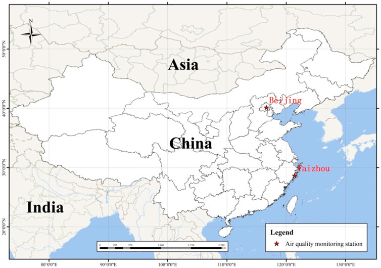
To verify the effectiveness of the proposed method on air quality prediction tasks, we adopt two real-world hourly air quality PM2.5 datasets to perform air quality prediction experiments. They are Beijing PM2.5 dataset (Liang et al., 2015), and Taizhou PM2.5 dataset. Figure 1 shows the location of Beijing and Taizhou air quality monitoring stations in China. In particular, Beijing city is located at $116°66^{\prime }$ east longitude and $40°13^{\prime }$ north latitude. Taizhou is located at $121°42^{\prime }$ east longitude and $28°65^{\prime }$ north latitude. Taizhou city lies in the southeast of Zhejiang Province, China. These two cities represent two distinct climate areas in China. Specially, Beijing city is a typical dry area in the north of China, whereas Taizhou city is a typical wet area in the south of China.

FIGURE 1

FIGURE 1. The location of Beijing and Taizhou air quality monitoring stations in China.

The used Beijing PM2.5 dataset contains around 43,800 samples, each of which was recorded with an hourly interval ranging from 01/01/2010 to 12/31/2014. In this dataset, the PM2.5 data (http://www.mee.gov.cn/) was collected from the United States Embassy in Beijing, and the corresponding meteorological data (http://tianqi.2345.com/) was collected from Beijing Capital International Airport. This dataset comprises of eight feature items, including PM2.5 concentration (ug/m³), dew point, temperature, pressure, combined wind direction, cumulated wind speed (m/s), cumulated hours of snow, cumulated hours of rain. Figure 2 presents an illustration of hourly PM2.5 values from 5/01/2014 to 5/31/2014 on Beijing PM2.5 dataset.

FIGURE 2

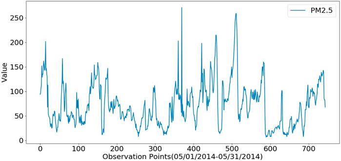
FIGURE 2. An illustration of hourly PM2.5 values (ug/m³) from 5/01/2014 to 5/31/2014 on Beijing PM2.5 dataset [Each observation point in the horizontal axis denotes a timescale (hour) related to the collected PM2.5 value, as described in the vertical axis in this figure].

The used Taizhou PM2.5 dataset contains about 26,000 hourly records ranging from 01/01/2017 to 12/31/2019. They were collected by our teams from the single Hongjia monitoring station, which is located in Jiaojiang urban district from Taizhou city in the southeast of Zhejiang Province. This dataset also include eight feature items, such as PM2.5 concentration (ug/m³), dew point, temperature, pressure, combined wind direction, cumulated wind speed (m/s), cumulated hours of rain, cumulated hours of relative humidity. Figure 3 provides an illustration of hourly PM2.5 values from 10/01/2019-10/31/2019 on Taizhou PM2.5 dataset.

FIGURE 3

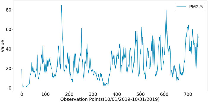
FIGURE 3. An illustration of hourly PM2.5 values (ug/m³) from 10/01/2019-10/31/2019 on Taizhou PM2.5 dataset [Each observation point in the horizontal axis denotes a timescale (hour) related to the collected PM2.5 value, as described in the vertical axis in this figure].

2.2 Method

Figure 4 presents an overview of our proposed temporal difference-based graph transformer networks (TDGTN) for air quality PM2.5 prediction. Like the original Transformer (Vaswani et al., 2017), our proposed TDGTN model comprises of encoder and decoder layers associated with the graph attention mechanism, as depicted in Figure 4. Compared with the original Transformer (Vaswani et al., 2017), TDGTN has two distinct properties. One is that we embed the graph attention into the encoder and decoder instead of the common multi-head attention in the original Transformer except for the used masked multi-head attention. The other is that based on time series PM2.5 data, the first-order backward difference information between two adjacent moments is embedded into the constructed graph so as to learn long-term dependency and complex relationships from a graph perspective. In the following, we will describe the relevant details of TDGTN.

FIGURE 4

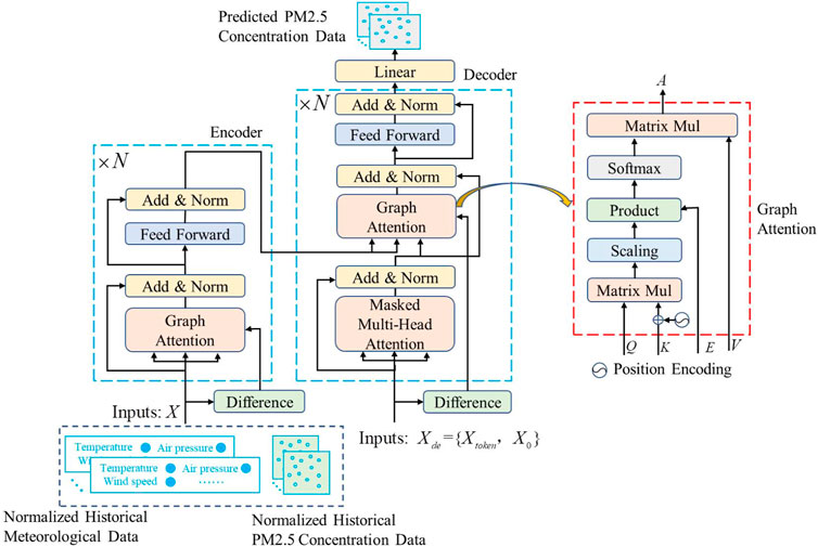
FIGURE 4. An overview of our proposed temporal difference-based graph transformer networks (TDGTN) for air quality PM2.5 prediction.

2.2.1 Problem Description

Given a length $L_x$ of input time series data $X=\left\{x_1\text{, }{x}_2,\dots ,x_{L_x}\right\}$ $\left(x_i\in R^{d_x}\right)$ with feature dimension $d_x$, the used air quality prediction methods aim to forecast the corresponding time series PM2.5 data $Y=\left\{y_1\text{, }{y}_2,\dots ,y_{L_y}\right\}$ $\left(y_i\in R^{d_y}\right)$ with a length $L_y$ and feature dimension $d_y$. The encoder aims to learn hidden continuous feature representations $Z=\left\{z_1\text{, }{z}_2,\dots ,z_{L_z}\right\}$ with a length $L_z$ from input time series data $X$. Then, the decoder produces an output of $Y=\left\{y_1\text{, }{y}_2,\dots ,y_{L_y}\right\}$ from the obtained hidden continuous feature representations in the encoder. This inference is performed by means of an step-by-step implementation, in which the decoder computes a new hidden feature representation $z_{k+1}$ from the previous feature representation $z_k$ and other outputs in $k$-th step, and then predict $\left(k+1\right)$-th time series data $y_{k+1}$.

2.2.2 Graph Construction

Graphs, as a special form of data, aim to characterize the relationships between different entities. GNNs endow each node in a graph with an ability of learning its neighborhood context by means of propagating information through graph-based structures. In this case, air quality PM2.5 prediction for the single air monitoring station can be intuitively regarded as a problem of graph-based multivariate time series forecasting from a view point of graphs. Considering the similarity of different time moments and the importance of temporal difference between two adjacent moments for air quality prediction, for the single air monitoring station we first construct graph-structured data from the obtained time series PM.25 data at different moments without explicit graph structure, as described below. Based on the constructed graph-structured data, modeling time series PM2.5 data from a graph prospective may be a good way to maintain their temporal trajectory while exploring the temporal dependencies among time series PM2.5 data.

A graph is defined as $G=\left(\Lambda ,\Gamma \right)$ where $\Lambda$ represents its nodes, and $\Gamma$ denotes its edges. The number of nodes in a graph is denoted by $n$. The graph adjacency matrix $U\in R^{n\times n}$ is used to characterize the relationships among nodes.

As shown in Figure 5, the moment $t_i$ $\left(i=\mathrm{1,2},\mathrm{...}n\right)$ from time series PM2.5 data can be regarded as the $i$-th node in a graph, and they are interconnected by using their hidden dependency relationships. Therefore, all the nodes in a graph can be defined as

$\mathrm{\Lambda }=\left(t_1,t_2,\cdots t_n\right)(1)$

FIGURE 5

FIGURE 5. (A) an illustration of constructing graph-structured data from time series PM2.5 data at four different moments, (B) the graph adjacency matrix is computed by using a Hadamard product $A\odot E$ between the attention scores $A$ and first-order backward difference matrix $E$.

The graph adjacency matrix is computed by a Hadamard product

$U=A\odot E(2)$

Where $A\in R^{n\times n}$ denotes the initial multiplicative attention scores calculated by $A=X{X}^{\prime }$, and $E\in R^{n\times n}$ represents the first-order backward difference matrix, which is obtained by

$E=E^{\prime }\cdot W(3)$

$E^{\prime }=\left({\nabla }_{10},{\nabla }_{21},{\nabla }_{32},\mathrm{...},{\nabla }_{n,n-1}\right)(4)$

${\nabla }_{i,i-1}=x_i-x_{i-1},i=\mathrm{1,2},\cdots ,n(5)$

Where $W$ is the linear transformation of the original first-order backward difference matrix $E^{\prime }\in R^{n\times 1}$, and ${\nabla }_{i,i-1}$ is the first-order backward difference between two adjacent nodes in a graph representing the meteorological dynamical changes between two adjacent moments. In this way, the edge values in $\Gamma$ from a graph correspond to the element values in the produced graph adjacency matrix $U$, as depicted in Figure 5A.

It’s worth pointing that there are two distinct properties about our constructed graph-structured data from original time series PM2.5 data without explicit graph structures. First, the attention score $A$ is used to weigh the similarity of different nodes (i.e., time moments). The higher the similarity of different nodes is, the larger the attention score values are. Moreover, the dynamical changing information in time series PM2.5 data between two adjacent moments is very important for air quality prediction. Therefore, the Hadamard product $A\odot E$ between the attention score $A$ and first-order backward difference matrix $E$ is designed to weigh the similarity of different nodes, and the dynamical changing in time series PM2.5 data simultaneously. Second, it is known that in long-term time series data the obtained information with close nodes (such as two neighboring nodes) is more important for air quality prediction than the obtained information with far nodes. Multiplying the attention scores of far nodes with the first-order backward difference of neighboring nodes, thus makes the graph adjacency matrix $U$ not only focuses on the information of far nodes, but also pays more attention to the neighboring nodes.

After constructing graph-structured data, the self-attention mechanism in Transformer (Vaswani et al., 2017) can be operated on these graph-structured data. Then, we improve the self-attention mechanism with the temporal difference information. This yields our graph attention mechanism used in the proposed TDGTN model for learning long-term temporal dependencies from a graph prospective on air quality PM2.5 prediction tasks.

2.2.3 The Details of TDGTN Model

Similar to the original Transformer (Vaswani et al., 2017), TDGTN contains encoder and decoder blocks with the developed graph attention mechanism, as described in Figure 4.

Encoder: The encoder is composed of a graph attention layer and a fully connected feed-forward network layer. Around each of two sub-layers, the residual connection (He et al., 2016) is adopted, each of them is followed by an addition and layer-normalization layer (Add and Norm). Given input time series data $X$, the encoder aims to learn the interrelationship of PM2.5 related data in time series data from a graph perspective.

Decoder: The decoder comprises of a masked multi-head attention layer, a graph attention layer and a fully connected feed-forward network layer, and each of them is followed by an addition and layer-normalization layer (Add and Norm). Similar to the encoder, the residual connection is employed around each of two sub-layers. The decoder accepts the input time series data $X_{de}=\left\{X_{token},X_0\right\}$, in which $X_{token}$ denotes the started tokens, and $X_0$ represents the placeholder for target time series data. The decoder aims to produce the output of predicted PM2.5 concentration data in a generative manner based on the obtained hidden continuous feature representations in the encoder.

Graph attention: Based on the constructed graph, we improve the self-attention mechanism with the temporal difference information and embed it into the produced graph-structured data to calculate the hidden representations of each node in the graph. As shown in (Vaswani et al., 2017), the canonical self-attention consists of three parts: query, key and value, and is computed by performing scaling dot product calculation:

$\mathrm{Attention}\left(Q,K,V\right)=\mathrm{softmax}\left(\frac{Q{K}^{{\rm T}}}{\sqrt{d}}\right)V(6)$

Where $Q\in R^{L\times d}$ is the query matrix, $K\in R^{L\times d}$ is the key matrix, $V\in R^{L\times d}$ is the value matrix, $L$ is the length of input data, and $d$ is the feature dimension of input data.

As mentioned-above, the first-order backward difference between two adjacent nodes in a graph can be used to represent the meteorological dynamical changes between two adjacent moments. This difference information is useful for air quality prediction, and can be embedded into the canonical self-attention. In order to simultaneously capture the interrelation and dynamical changes among different nodes, we modify the attention calculation in Eqn. 6 by multiplying the first-order backward difference matrix $E$ as follows:

$\mathrm{Attention}=\mathrm{softmax}\left(\left(\frac{Q\cdot K^{{\rm T}}}{\sqrt{d}}\right)\cdot E\right)V(7)$

For graph-based time series PM2.5 data prediction, we employed fixed position encoding with the nonlinear sine and cosine functions (Vaswani et al., 2017) to provide the temporal information of time series data for graph attention calculation.

3 Evaluation Criteria

To verify the performance of air quality PM2.5 prediction methods, three representative evaluation metrics, including mean absolute error (MAE), root mean square error (RMSE), and mean absolute percentage error (MAPE), were employed for experiments. MAE, RMSE, and MAPE are defined as:

$\mathrm{MAE}\left(y,\stackrel{\wedge }{y}\right)=\frac{1}{m}{\displaystyle \sum _{i=1}^m\left|y_i-\stackrel{\wedge }{y_i}\right|}(8)$

$\mathrm{RMSE}\left(y,\stackrel{\wedge }{y}\right)=\sqrt{\frac{1}{m}{\displaystyle \sum _{i=1}^m{\left(y_i-\stackrel{\wedge }{y_i}\right)}^2}}(9)$

$\mathrm{MAPE}\left(y,\stackrel{\wedge }{y}\right)=\frac{1}{m}{\displaystyle \sum _{i=1}^m\frac{\left|y_i-\stackrel{\wedge }{y_i}\right|}{y_i}}(10)$

Where $y$ and $\stackrel{\wedge }{y}$ separately denotes the ground-truth and predicted PM2.5 value, and $m$ represents the whole number of testing data. The smaller the values of MAE, RMSE, and MAPE are, the higher the final prediction results are. Since MAPE is very sensitive to outlier data, the obtained MAPE values are often higher than MAE and RMSE. In this case, MAE, RMSE and MAPE are employed simultaneously to evaluate the performance of all used methods.

3.1 Implementation Details

We implement all the experiments on a PC server with a GPU NVIDIA Quadro P6000 with 24G memory. The open source Pytorch tools are leveraged to conduct all machine learning models for air quality prediction. For deep learning models, the open source Tensorflow library is installed and configured. The Adam optimizer is adopted, and the initial learning rate is set to le-4. The batch size is set to 32, the maximum epoch number is 200, and the mean squared error loss function is employed. Normalization is conducted to be [0, 1] for air quality time series data. The lookup size (window size), which is used to represent historical observations as input size of all machine learning models, is 24 for its promising performance. We evaluate the performance of our method in comparison with other representative methods, such as the traditional ARMA and SVR, as well as the recently-emerged deep models like CNNs, LSTMs, original Transformer methods, as describe below.

ARMA is a traditional linear statistical method for time series data prediction. Here, ARMA is just used for singe-step air quality prediction since it is limited multi-step air quality prediction strategy. For ARMA, there are two key parameters ARMA (p, q) affecting its performance, in which p is the order of the AR part and q is the order of the MA part. In this work, we seek the optimal p and q in a simple exhausting search way in the range of [1, 10] with an interval of 1 to produce the best performance for ARMA. As a result, we separately employ ARMA (4, 1) on Beijing dataset and ARMA (1, 9) on Taizhou dataset for experiments due to its best performance. SVR is a kernel method on the basis of non-linear statistical machine learning theories. We adopt the linear kernel for SVR on air quality PM2.5 prediction tasks.

CNNs are a well-known deep model originally processing two-dimension (2D) image data. Due to the used 1D time-series PM2.5 data, 1D-CNN is adopted in this work. The network configuration for 1D-CNN is that it consists of 256 convolution kernels with a kernel width of 5 and a stride of 1. Then, a batch normalization layer, max-pooling layer, rectified linear units (RLU) layer, a dropout (0.3) layer, and a fully-connected (FC) layer are used after the convolution layers.

LSTMs are a typical kind of recurrent architecture modeling long-range dependencies of time series data. Bidirectional LSTM (BiLSTM) is employed for air quality prediction. BiLSTM contains a forward LSTM and a backward LSTM. We leveraged a two-layer BiLSTM for air quality forecasting in this work. Each layer of BiLSTM contains 256 hidden neurons, followed by a dropout (0.05) layer. For the original Transformer model (Vaswani et al., 2017) and our proposed TDGTN model, we leverage three encoders and two decoders for their promising performance on air quality PM2.5 prediction. Moreover, in these two Transformer-based models the number of multi-head attention is 8, and the used single feed-forward network has 2048 nodes.

In this work, we adopt a year-independent strategy for air quality forecasting experiments which is definitely close to the real-world sceneries. More specially, the training, and testing sets are selected from different years. In detail, on the used Beijing PM2.5 dataset, the first four-year data (01/01/2010 to 12/31/2013) is selected as the training net, and the last year data (01/01/2014-12/31/2014) is adopted for testing. On the used Taizhou PM2.5 dataset, the first two-year data (01/01/2017 to 12/31/2018) is employed for training, and the last year data (01/01/2019 to 12/31/2019) is adopted for testing. During the training of deep models, we randomly select 10% of the entire training set as the validation set for model validation.

3.2 Results and Analysis

To verify the performance of different air quality PM2.5 prediction methods, we presented two types of experimental results: single-step prediction for the next 1 h, and multi-step prediction for the next multiple hours.

3.2.1 Single-Step Prediction Results

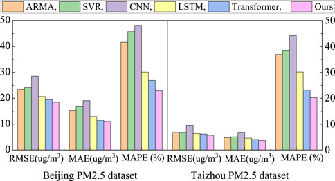
Figure 6 provides performance comparisons of different air quality prediction methods on Beijing and Taizhou PM2.5 datasets for single-step PM2.5 prediction tasks when the forward-step prediction size is 1 for the next 1 h (h1). These comparing methods contain ARMA, the linear SVR, CNN, LSTM, the original Transformer (abbreviated as Transformer), as well as our method. As shown in Figure 6, it can be seen that our method outperforms other used methods on Beijing and Taizhou PM2.5 datasets for single-step PM2.5 prediction tasks. In detail, our method obtains the lowest RSME, MAE, and MAPE on these two datasets. More specially, our method is able to reduce RMSE to 18.51 (ug/m³), MAE to 11.06 (ug/m³), and MAPE to 22.91 (%) on Beijing PM2.5 dataset, whereas on Taizhou PM2.5 dataset our method can reduce RMSE to 5.70 (ug/m³), MAE to 3.66 (ug/m3), and MAPE to 20.23 (%). This indicates the effectiveness of our proposed method for air quality PM2.5 prediction from a graph perspective. In comparison with other methods like ARMA, SVR, CNN, LSTM, and Transformer, our method has stronger capability of capturing long-term dependency and complex relationships from time series PM2.5 data for air quality prediction. In addition, our method yields better performance than Transformer, showing the advantages of our method on the basis of graph attention.

FIGURE 6

FIGURE 6. Comparisons of different methods for single-step PM2.5 prediction tasks for the next 1 h.

Besides, compared with traditional shallow learning methods like ARMA and SVR, deep learning methods, including LSTM, Transformer and our method, produce better performance for air quality prediction. This demonstrates the superiority of deep learning techniques over traditional shallow learning techniques on air quality prediction tasks. However, the used 1D-CNN obtains slight lower performance than SVR on single-step PM2.5 prediction tasks. This indicates that CNN may not very effective to learn long-term dependency and complex relationships from 1D time series PM2.5 data.

3.2.2 Multi-Step Prediction Results

For multi-step prediction results, we provided performance comparisons of different air quality prediction methods for the next multiple hours (6, 12, 24, 48). For the next 6 h, the average prediction results in the next forward 6 h were reported as the testing error of different methods. For more than the next 6 h, we divided them into a number of adjacent intervals and trained individual models corresponding to every interval. Then, we figured out the average prediction results for every interval. In particular, for the next 12 h prediction, we split it into three intervals: 0–3 h, 3–6 h, and 6–12 h. For the next 24 h prediction, we split it into four intervals: 0–3 h, 3–6 h, 6–12 h, and 12–24 h. For the next 48 h prediction, we split it into four intervals: 0–6 h, 6–12 h, 12–24 h and 24–48 h.

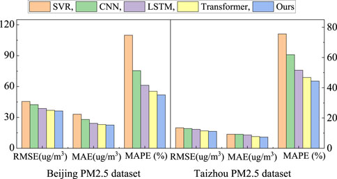
Figure 7 presents the obtained results (RMSE, MAE and MAPE) of different methods for the next 6 h on Beijing and Taizhou PM2.5 datasets. It can be seen from the results in Figure 7, compared with other methods, our method achieves the smaller RSME, MAE and MAPE on Beijing and Taizhou PM2.5 datasets. This indicates the superiority of the proposed method on long-term air quality prediction tasks. More specially, our method reduces RMSE to 36.27 (ug/m³), MAE to 22.61 (ug/m³), MAPE to 51.88 (%) on Beijing PM2.5 dataset, and RMSE to 11.19 (ug/m³), MAE to 7.40 (ug/m³), and MAPE to 44.37 (%) on Taizhou PM2.5 dataset, respectively. The ranking order for other methods is Transformer, LSTM, CNN, and SVR. Note that CNN provides slightly smaller RMSE, MAE, and MAPE than SVR on multi-step PM2.5 prediction tasks for the next 6 h. This is opposite to single-step PM2.5 prediction tasks for the next 1 h, as shown in Figure 6. This shows that CNN is capable of promoting the prediction performance with the increasing forward-step prediction size from the next 1 h to the next 6 h. This finding of CNN will be verified further in the next 12, 24 and 48 h.

FIGURE 7

FIGURE 7. Comparisons of different methods for multi-step prediction results for the next 6 h.

Figures 8, 9 separately show the prediction results (RMSE, MAE and MAPE) of different methods for the next 12 h (three intervals) on Beijing and Taizhou PM2.5 datasets. Figures 10, 11 individually depict the prediction results (RMSE, MAE and MAPE) of different methods for the next 24 h (four intervals) on Beijing and Taizhou PM2.5 datasets. Figures 12, 13 independently present the prediction results (RMSE, MAE and MAPE) of different methods for the next 48 h (four intervals) on Beijing and Taizhou PM2.5 datasets. From the results in Figures 8–13, we can observe that when the forward prediction size increases from 12 to 48 h, the multi-step PM2.5 prediction accuracies of all used methods clearly drop down. This may be attributed to the fact that the larger the forward prediction size is, the more difficult and challenging the accurate air quality prediction task is. In addition, Figures 8–13 show that our method still presents the lowest prediction error (RMSE, MAE, MAPE) among all used methods when the forward prediction size changes from 12 to 48 h. Besides, CNN performs better than SVR again for the next 12–48 h, and outperforms LSTM for the next 48 h. This shows that CNN is more appropriate to implement long-term air quality prediction compared with short-term air quality prediction tasks.

FIGURE 8

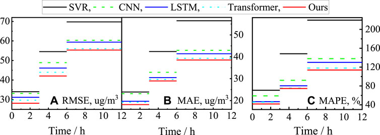
FIGURE 8. Comparisons of different methods for multi-step prediction results for the next 12 h on Beijing dataset.

FIGURE 9

FIGURE 9. Comparisons of different methods for multi-step prediction results for the next 12 h on Taizhou dataset.

FIGURE 10

FIGURE 10. Comparisons of different methods for multi-step prediction results for the next 24 h on Beijing dataset.

FIGURE 11

FIGURE 11. Comparisons of different methods for multi-step prediction results for the next 24 h on Taizhou dataset.

FIGURE 12

FIGURE 12. Comparisons of different methods for multi-step prediction results for the next 48 h on Beijing dataset.

FIGURE 13

FIGURE 13. Comparisons of different methods for multi-step prediction results for the next 48 h on Taizhou dataset.

To intuitively exhibit the superiority of our method over the original Transformer method, Figures 14, 15 separately provide the visualization of their single-step ground truth and predicted PM2.5 values for the next 1 h, and multi-step ground truth and predicted PM2.5 values for the next 48 h on Beijing and Taizhou PM2.5 datasets. The forward prediction size is 4/01/2014-4/30/2014 on Beijing PM2.5 dataset, and 4/01/2019-4/30/2019 on Taizhou PM2.5 dataset. Here, an illustration of their difference is labeled with a red circle in Figures 14, 15.

FIGURE 14

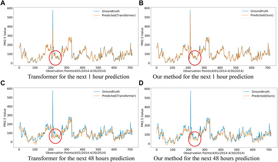
FIGURE 14. Comparisons of our method and Transformer on single-step (h1) and multi-step (h48) ground truth and air quality prediction tasks during 1 month (4/01/2014-4/30/2014) on Beijing dataset.

FIGURE 15

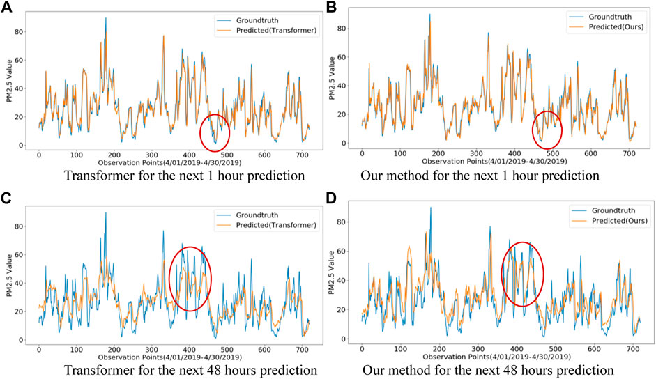
FIGURE 15. Comparisons of our method and Transformer on single-step (h1) and multi-step (h48) ground truth and air quality prediction tasks during 1 month (4/01/2019-4/30/2019) on Taizhou dataset.

As shown in Figures 14, 15, we can observe that both of them obtain promising performance on single-step prediction tasks for the next 1 h. Nevertheless, our method slightly outperforms Transformer on subtle changes in the time period of wave valley and the wave peak of air quality PM2.5 testing data from these two datasets. Moreover, such superiority of our method over Transformer is more obvious for multi-step prediction results for the next 48 h. The visualization in Figures 14, 15 show the advantages of our method over Transformer on short-term and long-term air quality PM2.5 prediction tasks, again.

Compared with the results obtained on single-step PM2.5 prediction tasks, all used methods for multi-step PM2.5 prediction achieves much larger RMSE, MAE and MAPE, demonstrating the difficulty in long-term air quality prediction when adopting a year-independent strategy widely used in real-word sceneries. Specially, the obtained MAPE values are much higher than RMSE, and MAE, due to the inherent drawback of MAPE as an error measure, that is, MAPE is very sensitive to outlier data (Kim and Kim, 2016). This is consistent with previous findings (Wen et al., 2019; Du et al., 2021). Nevertheless, the obtained results on multi-step PM2.5 prediction tasks demonstrate the advantage of the proposed TDGTN again, outperforming other methods.

4 Conclusion and Future Work

In this work, a new deep learning model called TDGTN is proposed to learn long-term temporal dependencies and complex relationships from time series PM2.5 data for air quality PM2.5 prediction. The proposed TDGTN model contains a number of encoder and decoder layers associated with the newly-developed graph attention mechanism. Specially, the conventional self-attention mechanism in the original Transformer model is improved by means of integrating the temporal difference information, which gives rise to a new graph attention mechanism used in the proposed TDGTN model. Based on the constructed graph-structured data, we are the first to implement air quality PM2.5 prediction tasks for the single air monitoring station from a view point of graphs. Experiment results on Beijing and Taizhou PM2.5 datasets demonstrate the promising performance of the proposed TDGTN method on both short-term and long-term air quality prediction tasks.

It is noted that for air quality prediction on different cities, all used machine learning methods should be trained according to the collected data corresponding to this city. Otherwise, their obtained air quality prediction performance is usually poor due to the distribution difference of collected data from different cities. This is an inherent drawback for all machine learning algorithms. To alleviate this problem, combining deep learning with transfer learning techniques (Wang L. et al., 2019) may be a possible solution for cross-city air quality prediction. Moreover, it is also interesting to exploit a physics-based method (Ponomarev et al., 2020) that is applicable over different locations or regions in future. Besides, this work focuses on air quality prediction on a single city (Beijing or Taizhou) rather than a special region with multiple cities. In particular, we aim to integrate the advantages of GNNs and Transformer techniques and evaluate their performance of air quality PM2.5 prediction from a single monitoring station in two cities. Considering the fact that GNNs are able to capture the spatial dependencies among multiple air quality monitoring stations, it is interesting to extend our model for a regional estimation of PM2.5 from multiple cities throughout the world. Additionally, the proposed method was designed for a single monitoring station from a single city, thereby failing to analyze the spatial variations. To address this issue, it is also meaningful for air quality prediction to incorporate satellite-based air pollution data (Xu et al., 2019) from satellite measurements, which can map air pollution for a broad region instead of a single city.

Data Availability Statement

The raw data supporting the conclusions of this article will be made available by the authors, without undue reservation.

Author Contributions

ZZ Conceptualization, Methodology, Software, Writing-Original draft. SZ: Conceptualization, Software. XZ: Project administration, Writing- Reviewing and Editing. LC and JY: Data collection, Pre-processing.

Funding

This work was supported by Zhejiang Provincial National Science Foundation of China under Grant No. LY20E080013, LZ20F020002, and National Science Foundation of China (NSFC) under Grant No. 61976149.

Conflict of Interest

The authors declare that the research was conducted in the absence of any commercial or financial relationships that could be construed as a potential conflict of interest.

Publisher’s Note

All claims expressed in this article are solely those of the authors and do not necessarily represent those of their affiliated organizations, or those of the publisher, the editors and the reviewers. Any product that may be evaluated in this article, or claim that may be made by its manufacturer, is not guaranteed or endorsed by the publisher.

References

Abirami, S., and Chitra, P. (2021). Regional Air Quality Forecasting Using Spatiotemporal Deep Learning. J. Clean. Prod. 283, 125341. doi:10.1016/j.jclepro.2020.125341

CrossRef Full Text | Google Scholar

Agarwal, S., Sharma, S., R., S., Rahman, M. H., Vranckx, S., Maiheu, B., et al. (2020). Air Quality Forecasting Using Artificial Neural Networks with Real Time Dynamic Error Correction in Highly Polluted Regions. Sci. Total Environ. 735, 139454. doi:10.1016/j.scitotenv.2020.139454

PubMed Abstract | CrossRef Full Text | Google Scholar

Aggarwal, A., and Toshniwal, D. (2021). A Hybrid Deep Learning Framework for Urban Air Quality Forecasting. J. Clean. Prod. 329, 129660. doi:10.1016/j.jclepro.2021.129660

CrossRef Full Text | Google Scholar

Arhami, M., Kamali, N., and Rajabi, M. M. (2013). Predicting Hourly Air Pollutant Levels Using Artificial Neural Networks Coupled with Uncertainty Analysis by Monte Carlo Simulations. Environ. Sci. Pollut. Res. 20 (7), 4777–4789. doi:10.1007/s11356-012-1451-6

CrossRef Full Text | Google Scholar

Bazi, Y., Bashmal, L., Rahhal, M. M. A., Dayil, R. A., and Ajlan, N. A. (2021). Vision Transformers for Remote Sensing Image Classification. Remote Sens. 13 (3), 516. doi:10.3390/rs13030516

CrossRef Full Text | Google Scholar

Cekim, H. O. (2020). Forecasting PM10 Concentrations Using Time Series Models: a Case of the Most Polluted Cities in Turkey. Environ. Sci. Pollut. Res. 27 (20), 25612–25624. doi:10.1007/s11356-020-08164-x

CrossRef Full Text | Google Scholar

Chang, Q., Zhang, H., and Zhao, Y. (2020). Ambient Air Pollution and Daily Hospital Admissions for Respiratory System-Related Diseases in a Heavy Polluted City in Northeast China. Environ. Sci. Pollut. Res. Int. 27, 10055–10064. doi:10.1007/s11356-020-07678-8

PubMed Abstract | CrossRef Full Text | Google Scholar

Chang, Y.-S., Abimannan, S., Chiao, H.-T., Lin, C.-Y., and Huang, Y.-P. (2020). An Ensemble Learning Based Hybrid Model and Framework for Air Pollution Forecasting. Environ. Sci. Pollut. Res. 27 (30), 38155–38168. doi:10.1007/s11356-020-09855-1

CrossRef Full Text | Google Scholar

Chen, L., Xu, J., Wu, B., Qian, Y., Du, Z., Li, Y., et al. (2021). Group-Aware Graph Neural Network for Nationwide City Air Quality Forecasting. Available at: https://arxiv.org/abs/2108.12238.

Google Scholar

Chu, J., Dong, Y., Han, X., Xie, J., Xu, X., and Xie, G. (2021). Short-term Prediction of Urban PM2.5 Based on a Hybrid Modified Variational Mode Decomposition and Support Vector Regression Model. Environ. Sci. Pollut. Res. 28 (1), 56–72. doi:10.1007/s11356-020-11065-8

CrossRef Full Text | Google Scholar

Chung, J., Gulcehre, C., Cho, K., and Bengio, Y. (2014). Empirical Evaluation of Gated Recurrent Neural Networks on Sequence Modeling. Available at: https://arxiv.org/abs/1412.3555.

Google Scholar

Darçın, M. (2014). Association between Air Quality and Quality of Life. Environ. Sci. Pollut. Res. 21 (3), 1954–1959. doi:10.1007/s11356-013-2101-3

CrossRef Full Text | Google Scholar

De Melo, W. C., Granger, E., and Hadid, A. (2019). “Depression Detection Based on Deep Distribution Learning,” in 2019 IEEE International Conference on Image Processing (ICIP), Taipei, Taiwan, 22-25 September 2019, 4544–4548. doi:10.1109/ICIP.2019.8803467

CrossRef Full Text | Google Scholar

Donnelly, A., Misstear, B., and Broderick, B. (2015). Real Time Air Quality Forecasting Using Integrated Parametric and Non-parametric Regression Techniques. Atmos. Environ. 103, 53–65. doi:10.1016/j.atmosenv.2014.12.011

CrossRef Full Text | Google Scholar

Du, S., Li, T., Yang, Y., and Horng, S.-J. (2021). Deep Air Quality Forecasting Using Hybrid Deep Learning Framework. IEEE Trans. Knowl. Data Eng. 33 (6), 2412–2424. doi:10.1109/tkde.2019.2954510

CrossRef Full Text | Google Scholar

Duke, B., Ahmed, A., Wolf, C., Aarabi, P., and Taylor, G. W. (2021). “Sstvos: Sparse Spatiotemporal Transformers for Video Object Segmentation,” in Proceedings of the IEEE/CVF Conference on Computer Vision and Pattern Recognition, Nashville, TN, USA, 20-25 June 2021, 5912–5921. doi:10.1109/CVPR46437.2021.00585

CrossRef Full Text | Google Scholar

Elman, J. L. (1990). Finding Structure in Time. Cognitive Sci. 14 (2), 179–211. doi:10.1207/s15516709cog1402_1

CrossRef Full Text | Google Scholar

Feng, X., Li, Q., Zhu, Y., Hou, J., Jin, L., and Wang, J. (2015). Artificial Neural Networks Forecasting of PM2.5 Pollution Using Air Mass Trajectory Based Geographic Model and Wavelet Transformation. Atmos. Environ. 107, 118–128. doi:10.1016/j.atmosenv.2015.02.030

CrossRef Full Text | Google Scholar

Gao, X., and Li, W. (2021). A Graph-Based LSTM Model for PM2.5 Forecasting. Atmos. Pollut. Res. 12 (9), 101150. doi:10.1016/j.apr.2021.101150

CrossRef Full Text | Google Scholar

Gariazzo, C., Carlino, G., Silibello, C., Renzi, M., Finardi, S., Pepe, N., et al. (2020). A Multi-City Air Pollution Population Exposure Study: Combined Use of Chemical-Transport and Random-Forest Models with Dynamic Population Data. Sci. Total Environ. 724, 138102. doi:10.1016/j.scitotenv.2020.138102

PubMed Abstract | CrossRef Full Text | Google Scholar

Geng, G., Zhang, Q., Martin, R. V., van Donkelaar, A., Huo, H., Che, H., et al. (2015). Estimating Long-Term PM2.5 Concentrations in China Using Satellite-Based Aerosol Optical Depth and a Chemical Transport Model. Remote Sens. Environ. 166, 262–270. doi:10.1016/j.rse.2015.05.016

CrossRef Full Text | Google Scholar

Graupe, D., Krause, D., and Moore, J. (1975). Identification of Autoregressive Moving-Average Parameters of Time Series. IEEE Trans. Autom. Contr. 20 (1), 104–107. doi:10.1109/tac.1975.1100855

CrossRef Full Text | Google Scholar

He, K., Zhang, X., Ren, S., and Sun, J. (2016). “Deep Residual Learning for Image Recognition,” in Proceedings of the IEEE conference on computer vision and pattern recognition, Las Vegas, NV, USA, 27-30 June 2016, 770–778. doi:10.1109/CVPR.2016.90

CrossRef Full Text | Google Scholar

Hinton, G. E., and Salakhutdinov, R. R. (2006). Reducing the Dimensionality of Data with Neural Networks. science 313 (5786), 504–507. doi:10.1126/science.1127647

PubMed Abstract | CrossRef Full Text | Google Scholar

Hochreiter, S., and Schmidhuber, J. (1997). Long Short-Term Memory. Neural Comput. 9 (8), 1735–1780. doi:10.1162/neco.1997.9.8.1735

PubMed Abstract | CrossRef Full Text | Google Scholar

Jian, L., Zhao, Y., Zhu, Y. P., Zhang, M. B., and Bertolatti, D. (2012). An Application of ARIMA Model to Predict Submicron Particle Concentrations from Meteorological Factors at a Busy Roadside in Hangzhou, China. Sci. Total Environ. 426, 336–345. doi:10.1016/j.scitotenv.2012.03.025

PubMed Abstract | CrossRef Full Text | Google Scholar

Jin, N., Zeng, Y., Yan, K., and Ji, Z. (2021). Multivariate Air Quality Forecasting with Nested Long Short Term Memory Neural Network. IEEE Trans. Ind. Inf. 17 (12), 8514–8522. doi:10.1109/tii.2021.3065425

CrossRef Full Text | Google Scholar

Ke, J., Zhang, J., and Tang, M. (2021). Does City Air Pollution Affect the Attitudes of Working Residents on Work, Government, and the City? an Examination of a Multi-Level Model with Subjective Well-Being as a Mediator. J. Clean. Prod. 295, 126250. doi:10.1016/j.jclepro.2021.126250

CrossRef Full Text | Google Scholar

Kim, S., and Kim, H. (2016). A New Metric of Absolute Percentage Error for Intermittent Demand Forecasts. Int. J. Forecast. 32 (3), 669–679. doi:10.1016/j.ijforecast.2015.12.003

CrossRef Full Text | Google Scholar

Kipf, T. N., and Welling, M. (2016). Semi-supervised Classification with Graph Convolutional Networks. Available at: https://arxiv.org/abs/1609.02907.

Google Scholar

Lanchantin, J., Wang, T., Ordonez, V., and Qi, Y. (2021). “General Multi-Label Image Classification with Transformers,” in Proceedings of the IEEE/CVF Conference on Computer Vision and Pattern Recognition, Nashville, TN, USA, 20-25 June 2021, 16478–16488. doi:10.1109/cvpr46437.2021.01621

CrossRef Full Text | Google Scholar

LeCun, Y., Bengio, Y., and Hinton, G. (2015). Deep Learning. Nature 521 (7553), 436–444. doi:10.1038/nature14539

PubMed Abstract | CrossRef Full Text | Google Scholar

Lee, H.-M., Park, R. J., Henze, D. K., Lee, S., Shim, C., Shin, H.-J., et al. (2017). PM2.5 Source Attribution for Seoul in May from 2009 to 2013 Using GEOS-Chem and its Adjoint Model. Environ. Pollut. 221, 377–384. doi:10.1016/j.envpol.2016.11.088

PubMed Abstract | CrossRef Full Text | Google Scholar

Liang, X., Zou, T., Guo, B., Li, S., Zhang, H., Zhang, S., et al. (2015). Assessing Beijing's PM 2.5 Pollution: Severity, Weather Impact, APEC and Winter Heating. Proc. R. Soc. A 471 (2182), 20150257. doi:10.1098/rspa.2015.0257

CrossRef Full Text | Google Scholar

Liao, Q., Zhu, M., Wu, L., Pan, X., Tang, X., and Wang, Z. (2020). Deep Learning for Air Quality Forecasts: a Review. Curr. Pollut. Rep. 6 (4), 399–409. doi:10.1007/s40726-020-00159-z

CrossRef Full Text | Google Scholar

Liu, H., Yan, G., Duan, Z., and Chen, C. (2021). Intelligent Modeling Strategies for Forecasting Air Quality Time Series: A Review. Appl. Soft Comput. 102, 106957. doi:10.1016/j.asoc.2020.106957

CrossRef Full Text | Google Scholar

Mihailovic, D. T., Alapaty, K., and Podrascanin, Z. (2009). Chemical Transport Models. Environ. Sci. Pollut. Res. 16 (2), 144–151. doi:10.1007/s11356-008-0086-0

CrossRef Full Text | Google Scholar

Neishi, M., and Yoshinaga, N. (2019). “On the Relation between Position Information and Sentence Length in Neural Machine Translation,” in Proceedings of the 23rd Conference on Computational Natural Language Learning (CoNLL), Hong Kong, China, November 3–4, 2019, 328–338. doi:10.18653/v1/k19-1031

CrossRef Full Text | Google Scholar

Niu, Z., Zhong, G., and Yu, H. (2021). A Review on the Attention Mechanism of Deep Learning. Neurocomputing 452, 48–62. doi:10.1016/j.neucom.2021.03.091

CrossRef Full Text | Google Scholar

Pak, U., Ma, J., Ryu, U., Ryom, K., Juhyok, U., Pak, K., et al. (2020). Deep Learning-Based PM2.5 Prediction Considering the Spatiotemporal Correlations: A Case Study of Beijing, China. Sci. Total Environ. 699, 133561. doi:10.1016/j.scitotenv.2019.07.367

PubMed Abstract | CrossRef Full Text | Google Scholar

Ponomarev, N. A., Elansky, N. F., Kirsanov, A. A., Postylyakov, O. V., Borovski, A. N., and Verevkin, Y. M. (2020). Application of Atmospheric Chemical Transport Models to Validation of Pollutant Emissions in Moscow. Atmos. Ocean. Opt. 33 (4), 362–371. doi:10.1134/s1024856020040090

CrossRef Full Text | Google Scholar

Pouyanfar, S., Sadiq, S., Yan, Y., Tian, H., Tao, Y., Reyes, M. P., et al. (2018). A Survey on Deep Learning: Algorithms, Techniques, and Applications. ACM Comput. Surv. (CSUR) 51 (5), 1–36. doi:10.1145/3234150

CrossRef Full Text | Google Scholar

Powers, J. G., Klemp, J. B., Skamarock, W. C., Davis, C. A., Dudhia, J., Gill, D. O., et al. (2017). The Weather Research and Forecasting Model: Overview, System Efforts, and Future Directions. Bull. Am. Meteorological Soc. 98 (8), 1717–1737. doi:10.1175/bams-d-15-00308.1

CrossRef Full Text | Google Scholar

Ragab, M. G., Abdulkadir, S. J., Aziz, N., Al-Tashi, Q., Alyousifi, Y., Alhussian, H., et al. (2020). A Novel One-Dimensional CNN with Exponential Adaptive Gradients for Air Pollution Index Prediction. Sustainability 12 (23), 10090. doi:10.3390/su122310090

CrossRef Full Text | Google Scholar

Saini, T., Chaturvedi, P., and Dutt, V. (2021). Modelling Particulate Matter Using Multivariate and Multistep Recurrent Neural Networks. Front. Environ. Sci. 614. doi:10.3389/fenvs.2021.752318

CrossRef Full Text | Google Scholar

Scarselli, F., Gori, M., Tsoi, A. C., Hagenbuchner, M., and Monfardini, G. (2008). The Graph Neural Network Model. IEEE Trans. Neural Netw. 20 (1), 61–80. doi:10.1109/TNN.2008.2005605

PubMed Abstract | CrossRef Full Text | Google Scholar

Schwartz, J. (1993). Particulate Air Pollution and Chronic Respiratory Disease. Environ. Res. 62 (1), 7–13. doi:10.1006/enrs.1993.1083

PubMed Abstract | CrossRef Full Text | Google Scholar

Seng, D., Zhang, Q., Zhang, X., Chen, G., and Chen, X. (2021). Spatiotemporal Prediction of Air Quality Based on LSTM Neural Network. Alexandria Eng. J. 60 (2). doi:10.1016/j.aej.2020.12.009

CrossRef Full Text | Google Scholar

Suleiman, A., Tight, M. R., and Quinn, A. D. (2019). Applying Machine Learning Methods in Managing Urban Concentrations of Traffic-Related Particulate Matter (PM10 and PM2.5). Atmos. Pollut. Res. 10 (1), 134–144. doi:10.1016/j.apr.2018.07.001

CrossRef Full Text | Google Scholar

Vaswani, A., Shazeer, N., Parmar, N., Uszkoreit, J., Jones, L., Gomez, A. N., et al. (2017). “Attention Is All You Need,” in Advances in Neural Information Processing Systems, 5998–6008.

Google Scholar

Wang, J., Bai, L., Wang, S., and Wang, C. (2019). Research and Application of the Hybrid Forecasting Model Based on Secondary Denoising and Multi-Objective Optimization for Air Pollution Early Warning System. J. Clean. Prod. 234, 54–70. doi:10.1016/j.jclepro.2019.06.201

CrossRef Full Text | Google Scholar

Wang, L., Geng, X., Ma, X., Liu, F., and Yang, Q. (2019). “Cross-city Transfer Learning for Deep Spatio-Temporal Prediction,” in Proceedings of the 28th International Joint Conference on Artificial Intelligence (IJCAI), Macao, China, August 10–16, 2019, 1893–1899. doi:10.24963/ijcai.2019/262

CrossRef Full Text | Google Scholar

Wang, W., Zhao, S., Jiao, L., Taylor, M., Zhang, B., Xu, G., et al. (2019). Estimation of PM2.5 Concentrations in China Using a Spatial Back Propagation Neural Network. Sci. Rep. 9 (1), 13788–13810. doi:10.1038/s41598-019-50177-1

PubMed Abstract | CrossRef Full Text | Google Scholar

Wen, C., Liu, S., Yao, X., Peng, L., Li, X., Hu, Y., et al. (2019). A Novel Spatiotemporal Convolutional Long Short-Term Neural Network for Air Pollution Prediction. Sci. total Environ. 654, 1091–1099. doi:10.1016/j.scitotenv.2018.11.086

PubMed Abstract | CrossRef Full Text | Google Scholar

Xiao, Q., Chang, H. H., Geng, G., and Liu, Y. (2018). An Ensemble Machine-Learning Model to Predict Historical PM2.5 Concentrations in China from Satellite Data. Environ. Sci. Technol. 52 (22), 13260–13269. doi:10.1021/acs.est.8b02917

PubMed Abstract | CrossRef Full Text | Google Scholar

Xu, H., Bechle, M. J., Wang, M., Szpiro, A. A., Vedal, S., Bai, Y., et al. (2019). National PM2.5 and NO2 Exposure Models for China Based on Land Use Regression, Satellite Measurements, and Universal Kriging. Sci. Total Environ. 655, 423–433. doi:10.1016/j.scitotenv.2018.11.125

PubMed Abstract | CrossRef Full Text | Google Scholar

Xu, J., Chen, L., Lv, M., Zhan, C., Chen, S., and Chang, J. (2021). HighAir: A Hierarchical Graph Neural Network-Based Air Quality Forecasting Method. Available at: https://arxiv.org/abs/2101.04264.

Google Scholar

Yan, X., Zang, Z., Luo, N., Jiang, Y., and Li, Z. (2020). New Interpretable Deep Learning Model to Monitor Real-Time PM2.5 Concentrations from Satellite Data. Environ. Int. 144, 106060. doi:10.1016/j.envint.2020.106060

PubMed Abstract | CrossRef Full Text | Google Scholar

Yang, W., Deng, M., Xu, F., and Wang, H. (2018). Prediction of Hourly PM2.5 Using a Space-Time Support Vector Regression Model. Atmos. Environ. 181, 12–19. doi:10.1016/j.atmosenv.2018.03.015

CrossRef Full Text | Google Scholar

Yue, Z., Witzig, C. R., Jorde, D., and Jacobsen, H.-A. (2020). “BERT4NILM: A Bidirectional Transformer Model for Non-intrusive Load Monitoring,” in Proceedings of the 5th International Workshop on Non-Intrusive Load Monitoring, Virtual conference, November 18, 2020, 89–93.

Google Scholar

Zaini, N. a., Ean, L. W., Ahmed, A. N., and Malek, M. A. (2021). A Systematic Literature Review of Deep Learning Neural Network for Time Series Air Quality Forecasting. Environ. Sci. Pollut. Res. 29, 4958–4990. doi:10.1007/s11356-021-17442-1

CrossRef Full Text | Google Scholar

Zhang, B., Wu, B., and Liu, J. (2020). PM2.5 Pollution-Related Health Effects and Willingness to Pay for Improved Air Quality: Evidence from China's Prefecture-Level Cities. J. Clean. Prod. 273, 122876. doi:10.1016/j.jclepro.2020.122876

CrossRef Full Text | Google Scholar

Zhang, H., Chen, G., Hu, J., Chen, S.-H., Wiedinmyer, C., Kleeman, M., et al. (2014). Evaluation of a Seven-Year Air Quality Simulation Using the Weather Research and Forecasting (WRF)/Community Multiscale Air Quality (CMAQ) Models in the Eastern United States. Sci. Total Environ. 473-474, 275–285. doi:10.1016/j.scitotenv.2013.11.121

PubMed Abstract | CrossRef Full Text | Google Scholar

Zhang, K., Thé, J., Xie, G., and Yu, H. (2020). Multi-step Ahead Forecasting of Regional Air Quality Using Spatial-Temporal Deep Neural Networks: A Case Study of Huaihai Economic Zone. J. Clean. Prod. 277, 123231. doi:10.1016/j.jclepro.2020.123231

CrossRef Full Text | Google Scholar

Zhang, Z., Zeng, Y., and Yan, K. (2021). A Hybrid Deep Learning Technology for PM2.5 Air Quality Forecasting. Environ. Sci. Pollut. Res. 28 (29), 39409–39422. doi:10.1007/s11356-021-12657-8

CrossRef Full Text | Google Scholar

Zhou, H., Zhang, S., Peng, J., Zhang, S., Li, J., Xiong, H., et al. (2021). “Informer: Beyond Efficient Transformer for Long Sequence Time-Series Forecasting,” in Proceedings of AAAI, Virtual conference, February 2–9, 2021, 11106–11115.

Google Scholar

Zhou, Q., Jiang, H., Wang, J., and Zhou, J. (2014). A Hybrid Model for PM 2.5 Forecasting Based on Ensemble Empirical Mode Decomposition and a General Regression Neural Network. Sci. Total Environ. 496, 264–274. doi:10.1016/j.scitotenv.2014.07.051

PubMed Abstract | CrossRef Full Text | Google Scholar