Boosted Regression Tree Algorithm for the Reconstruction of GRACE-Based Terrestrial Water Storage Anomalies in the Yangtze River Basin

The terrestrial water storage anomaly (TWSA) from the previous Gravity Recovery and Climate Experiment (GRACE) covers a relatively short period (15 years) with several missing periods. This study explores the boosted regression trees (BRT) and the artificial neural network (ANN) to reconstruct the TWSA series between 1982 and 2014 over the Yangtze River basin (YRB). Both algorithms are trained with several hydro-climatic variables (e.g., precipitation, soil moisture, and temperature) and climate indices for the YRB. The results from this study show that the BRT is capable of reconstructing TWSA and shows Nash–Sutcliffe efficiency (NSE) of 0.89 and a root-mean-square error (RMSE) of 18.94 mm during the test stage, outperforming ANN in about 2.3% and 7.4%, respectively. As a step further, the reliability of this technique in reconstructing TWSA beyond the GRACE era was also evaluated. Hence, a closed-loop simulation using the artificial TWSA series over 1982–2014 under the same scenarios for the actual GRACE data shows that BRT can predict TWSA (NSE of 0.92 and RMSE of 6.93 mm). Again, the BRT outperformed the ANN by approximately 1.1% and 5.3%, respectively. This study provides a new perspective for reconstructing and filling the gaps in the GRACE–TWSA series over data-scarce regions, which is desired for hydrological drought characterization and environmental studies. BRT offers such an opportunity for the GRACE Follow-On mission to predict 11 months of missing TWSA data by relying on a limited number of predictive variables, hence being adjudged to be more economical than the ANN.

1 Introduction

The terrestrial water storage anomaly (TWSA) from the observations of the preceding Gravity Recovery and Climate Experiment (GRACE) and the contemporary follow-one (GRACE-FO) missions is the sum of the water stored as snow/ice, surface waters, soil moisture, groundwater, and biomass. It is assumed to be concentrated on a virtual layer of water thickness at the Earth’s surface (Ferreira et al., 2020b). TWSA is a critical component of the hydrologic cycle, and thus, an instrumental dataset that underpins our understanding of water availability on different spatial scales and how its variability is affected by climate change and anthropogenic activities. Consequently, the monthly fields of TWSA have been used globally in hydrological studies to provide essential outcomes such as identifying key drivers of land water storage across the globe (Rodell et al., 2018). For example, a GRACE hydrological assessment over North India, as was undertaken by Rodell et al. (2009), highlighted the unsustainable consumption of groundwater for irrigation and other anthropogenic uses. While this assessment was revisited by Long et al. (2016), the combined impacts of climate variability and human water management on freshwater stocks across several continents have been detailed (see, e.g., Ahmed et al., 2014; Ndehedehe and Ferreira, 2020). Also notable is the work of Reager et al. (2014), who investigated the suitability of GRACE observations to infer the flood potential of various river basins at a lead time of several months. Indeed, GRACE applications are varied and transdisciplinary. This includes the possibility of estimating the evapotranspiration (Rodell et al., 2004a), river discharge (Syed et al., 2005) over data-poor regions, estimating water mass changes over permafrost regions (Velicogna et al., 2012), and data assimilations to improve the outputs of hydrological models (Zaitchik et al., 2008). Despite the importance of the TWSA datasets retrieved from the GRACE mission in hydrological studies, the relatively short period of approximately 20 years which contain a 11-month gap between the GRACE and GRACE-FO missions pose a challenge to an accurate assessment of key hydrological metrics. In particular, several gaps due to the lack of reliable measurements constrain the full potential of TWSA in, for example, drought studies and understanding the pace of climate change (e.g., Vishwakarma, 2020).

Several studies have attempted to reconstruct the TWSA series to cover long-term periods relying on different methods. For instance, Li et al. (2021) incorporated machine learning, analysis of time series, with techniques of statistical decomposition to globally reconstruct TWSA fields from 1979 to 2020. Wang et al. (2021) combined the GRACE data with soil moisture, precipitation, evapotranspiration, and temperature to reconstruct a long-term TWSA based on an extended short-term memory model. A simple linear version combining TWSA above the Amazon together with sea surface temperature (SST) indices has additionally been proposed (de Linage et al., 2014). Utilizing GRACE-derived TWSA and in situ river discharge data, Becker et al. (2011) applied a principal component analysis, which makes a linear and steady time-series supposition, to reconstruct GRACE–TWSA from 1980 to 2008 over the Amazon Basin. Other approaches include the use of an autoregressive model with the independent component analysis to predict TWSA in West Africa incorporating precipitation records and SST indices (Forootan et al., 2014b). However, this autoregressive version assumes a constant status of TWSA over the area and the prediction accuracy decreases after a 2-year forecast length. The water balance approach has also been applied to increase the TWSA series back to 1980 (cf. Yin et al., 2019). This approach uses multi-source datasets as inputs in the terrestrial water budget equation. All examples mentioned here require the use of mathematical models. It must be mentioned that the formulation of these techniques, which is primarily based on experimental datasets, and the rise in performance, has frequently been undertaken by way of increased model complexity, and the manner that they come to decisions, makes them a pattern/machine learning recognition problem (Wilby et al., 2003).

There is no mathematical model that can efficiently describe hydrological phenomena (cf. Mukhopadhyay, 2003). However, algorithms that make supposition(s) of the time-series with adaptive abilities provide an excellent alternative to predict the TWSA fields over a region. Consequently, many studies have explored the feasibility of artificial neural networks (ANNs) to reconstruct the TWSA series due to their ability to model linear and non-linear systems based on learning and prediction algorithms (Ahmed et al., 2019). ANN extracts complex relationships between model inputs and targets and builds complex and non-linear relationships that are robust as a forecasting tool for hydrological variables. For instance, extended TWSA time- series using an ANN approach to examine the long-term hydrological properties of TWSA have been investigated by several authors (see, e.g., Long et al., 2014; Zhang et al., 2016; Mukherjee and Ramachandran, 2018; Ferreira et al., 2019; Ahmed et al., 2019; Chen et al., 2019, and references therein). Overall, these studies agreed that the ANN’s performance improved when climatic observations were integrated with the GRACE–TWSA datasets. Nevertheless, this might be a disadvantage since the accuracy of the reconstruction depends a lot on data availability, especially for architectures with many layers. For many regions and river basins, this might impose limitations in using ANN. As a result, economical methods that can still faithfully reconstruct actual observations would be preferable, especially over data-poor regions. The present study proposes the use of a new approach, the boosted regression tree (BRT) technique to reconstruct the TWSA series.

The BRT technique depends on the insights and methodologies of both statistical and machine-learning approaches. This method varies mainly from conventional regression strategies, which produce a single excellent model, rather than utilizing the boosting approach to adaptively combine a large number of several simple tree models to improve the predictive process (Elith et al., 2006; Leathwick et al., 2006; Leathwick et al., 2008). The boosting process utilized in BRT locates its origins within machine learning (Schapire, 2003). However, posterior evolutions within the society of statistics re-explain it as a developed type of regression (Friedman et al., 2000). BRT has many vital benefits of tree-based strategies: 1) it could be used with an assortment type of response (binomial, Gaussian, and Poisson) through specifying the distribution of the error and the link function; 2) it contains a probabilistic or random component, which improves predictive performance, decreasing the definitive model variance through the use of just a random data subset to adequate every new tree (Friedman, 2002); 3) the algorithm automatically detects the best fit; 4) the model shows the impact of each predictor on the reconstruction after accounting for their overall contributions; and 5) the algorithm is robust and unaffected by missing values and outliers (Abeare, 2009). Fitting numerous trees in BRT overcomes the most significant obstacle of single tree models (i.e., their comparatively weak prediction achievement). BRT models are complicated; however, they can be concise in forms which provide a robust hydrological perception. Thereby, BRT is suitable for many environmental applications as well.

The main aim of this study is to evaluate the use of BRT to reconstruct the TWSA series of the Yangtze River basin (YRB), China. So far, BRT has been used only in groundwater level prognosis (Rahman et al., 2020; Sharafati et al., 2020) and, as far as we know, this study presents the first application of BRT to fill the missing gaps in the GRACE-derived TWSA. Furthermore, a comparison of the performance of BRT and ANN techniques has not been attempted in recent few studies that focused on TWSA reconstruction. Therefore, the focus of this study is to generate a continuous and uninterrupted TWSA series and develop a robust predictive technique that can backcast TWSA to address the hydrological and environmental problems over a given river basin. Furthermore, this study compares BRT outputs with those from a non-linear–autoregressive neural network with exogenous inputs (NARX) to define the most accurate method. Due to the nature of GRACE–TWSA, it has a statistical and physical relationship with the hydro-climatic variables (e.g., precipitation and soil moisture). For instance, Mo et al. (2016) found a strong correlation between precipitation and TWSA in southern China. Also, the availability of TWSA affects evapotranspiration and runoff (ibid). Ma et al. (2017) indicated that GRACE observations and Climate Change Initiative Soil Moisture could be used as significant indices of the spatial allocation of the drought procedure and its effect on the environment and local communities. This could improve water resource management and the early detection and monitoring of droughts. Consequently, the present study also uses a comprehensive and different data spectrum, replicating the dynamics in the energy and water cycles that affect TWSA for training the network over the YRB. Hence, the performance of the BRT model is the focus of the analyses, whilst also assessing the relative importance of the predictors used to reconstruct the TWSA.

2 Study Area

The Yangtze River is the longest in Asia, with a length of approx. 6,397 km. It flows from the Tibetan Plateau and runs through Qinghai, then turns south to Sichuan and Tibet; after that, it reaches Yunnan, Chongqing, and continues to Hubei, Hunan, running through Jiangxi, Anhui, and Jiangsu, and then emptying into the East China Sea near Shanghai. Its basin (hereafter YRB), extends for about 3,200 km from west to east and more than 1,000 km from north to south and drains an area of 1.8 × 10⁶ km², nearly one-fifth of the total land area of China (Figure 1). The YRB has succumbed to considerable modifications in climate and land cover/use, including the largest hydroelectric power station in the world (Three Gorges Dam—TGD). The TGD’s reservoir is the most vital anthropogenic feature in the YRB. It extends for 2.3 km with 185 m in height.

FIGURE 1

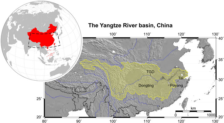
FIGURE 1. Location map of the Yangtze River basin, China, and its main surface waters. Source: adapted from Ferreira et al. (2020a).

The Yangtze River is very famous and has a significant role in China’s development of its economy, agriculture, tourism, transportation, culture, etc. Albeit for climate and water resource fields, the Qingling Mountain and Huaihe River are the more commonly recognized borders between northern and southern China. The Yangtze River is also perceived as the north–south boundary, at least from a cultural perspective. The climate in the north of the Yangtze River is dry with low temperatures and light rain, whereas, in the south, the climate is humid and warm with sufficient rainfall. Climate variation, floods and drought events, and irrigation have profoundly affected the water resources, bringing significant impacts on humans and nature. Three severe catastrophic floods happened in the YRB in 1931, 1956, and 1998. Although catastrophic floods like these have not happened in the YRB since the beginning of the 21st century, the YRB has faced a lot of medium and small floods. For instance, eight drought events have been identified in the YRB during the GRACE era, with three major droughts occurring in 2004, 2006, and 2011 (Sun et al., 2018).

3 Materials and Methods

3.1 Datasets

3.1.1 Global Precipitation Climatology Centre Precipitation

The Global Precipitation Climatology Centre (GPCC) was established in 1989 at the request of the World Meteorological Organization (WMO). The National Meteorological Service of Germany runs it as a German contribution to the World Climate Research Program. GPCC’s delegation is the worldwide analysis of monthly and daily precipitation on the Earth’s land surface based on in situ rain gauge data.

The monthly GPCC data, specifically, the GPCC–MP, gridded at a spatial resolution of 1° were used in this study due to its long-term record. The series starts from 1982, offering sufficient data for long-time period studies, and is based on the monthly records acquired by the Global Telecommunication System (GTS) of the WMO from about 7,000 to 9,000 stations (after high-level quality control). Generally, the GPCC–MP is known as the best in situ and GTS-based monthly land–surface precipitation reference product publicly available. To ensure the consistency of the time-series and reveal errors in the station metadata, the harmonization of station metadata and a sophisticated quality control is critical for GPCC to integrate several datasets. The data were retrieved from an online database, and further information is available at Schneider et al. (2013). The particular choice for this product is supported by the assessment and investigations carried out by Yu et al. (2020) over mainland China.

3.1.2 ERA-Interim Data System

To model the response of TWSA to evapotranspiration and temperature changes, instantaneous moisture flux (IE, equivalent to evapotranspiration), surface temperature (soil temperature level 1—SMTL1), soil temperature level 2/3/4 (SMTL2, SMTL3, and SMTL4), and 2-meter temperature (T2m) fields were retrieved from the ERA-Interim data system. These datasets were all obtained at a monthly temporal interval and gridded at a spatial resolution of 1°. The long-term consistency was the motivation to select the ERA-Interim reanalysis data for this study (cf. Forootan et al., 2014a).

3.1.3 GLDAS–Noah and GLDAS–Variable Infiltration Capacity

Soil moisture (the aggregate of all the layers from 0 to 2 m in depth), canopy, and snow storages from Global Land Data Assimilation Systems (GLDAS, Rodell et al., 2004b) driven by Noah in its version 2, which covers the period from 1948 to 2015, was used in this study as a predictor. We choose these data due to their availability over long periods. GLDAS–Noah version 2 datasets consist of 1° gridded data with a temporal resolution of 1 month.

For evaluating the performance of the BRT and ANN models, a closed-loop simulation using “independent” TWSA datasets from the GLDAS drive Variable Infiltration Capacity (VIC) land surface model L4, version 2, was considered. The GLDAS–VIC monthly product consists of 1° gridded data covering the period 1948 to 2015. These data were chosen due to their availability over long periods. Moreover, the GLDAS–VIC model creates the simulation outcomes that are nearest to the in situ data, and it additionally has the lowest dispersions and bias error values compared with other GLDAS streams.

3.1.4 Climate Indices

To model the response of YRB to the ENSO phenomenon, Bivariate ENSO Time-series (BEST, cf. Smith and Sardeshmukh, 2000), which is derived from the Southern Oscillation Index (SOI) and Niño 3.4 was used. The BEST index incorporates the oceanic (Niño 3.4) and atmospheric (SOI) components of ENSO processes into a particular field, and therefore, gives a more accurate description of the phenomenon. The time-series of worldwide temperature anomalies was also utilized to simulate the impact of global warming on TWSA variability, as shown by Dong et al. (2019). Over the YRB, it has been shown that the correlation between the eco-flow metrics and selected de-trended climate indices is strong, particularly for the synchronous Northern Hemisphere and Indian Ocean Dipole indices, as further explained by Dong et al. (2019). Moreover, these authors (ibid) indicated that the seasonal streamflow correlated more with selected climate indices than the annual streamflow. Thereby, the reconstruction of TWSA over the YRB also needs to consider such climate indices as predictors.

3.1.5 Gravity Recovery and Climate Experiment–Terrestrial Water Storage Anomaly Series

The GRACE-derived TWSA datasets used on this study are the so-called Level-3 products (Landerer and Swenson, 2012). They comprise monthly gridded values at a spatial resolution of 1°-by-1° based on the spherical harmonic coefficients provided by the Center for Space Research (CSR). All details regarding the processing procedures and caveats are available in the company publication by Landerer and Swenson (2012). Albeit TWSA fields were synthesized at a spatial resolution of 1°-by-1°, they are still limited to the nominal resolution of GRACE, which is 3°-by-3°. Nevertheless, scaling factors such as those computed by Landerer and Swenson (2012) can be used to improve the spatial resolution of GRACE–TWSA to 1°-by-1°. The scale factor used is the one computed by Long et al. (2015). To this end, the TWSA monthly grids refer to a temporal baseline of 2004–2009 at which the mean was subtracted.

The temporal time mean was also removed from the respective datasets (Sections 3.1.1–3.1.4) for the period 2004–2009. Figure 2 shows the correlation coefficient between TWSA and the predictors described in the aforementioned sub-sections. Overall, there is a good correspondence between TWSA and SM (0.887), and TWSA and P (0.612).

FIGURE 2

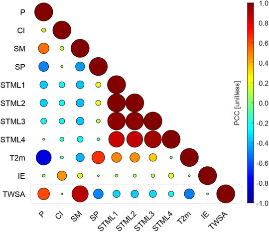
FIGURE 2. Pearson correlation coefficients (PCCs) between TWSA and the predictors described at Sections 3.1.1–3.1.4.

3.2 Methods

The methodological approach implemented in this study consists of the steps summarized in Figure 3 and is further described in the following sub-sections.

FIGURE 3

FIGURE 3. Flowchart of the primary process steps to reconstruct the GRACE-derived terrestrial water storage anomaly (TWSA) based on BRT and ANN (NARX) algorithms. The flowchart also shows the steps necessary for evaluating the reliability of the reconstructions using GLDAS–VIC-simulated TWSA.

3.2.1 Boosted Regression Tree

BRT, also known as stochastic gradient boosting, is one of many techniques that aims to enhance the performance and precision of the prediction of a single model by fitting several models and combining them to get the best prediction. The ability of the BRT method to enhance precision is based on the assumption that it is more straightforward to find and average many rough prediction rules other than to obtain a single high-precision prediction rule (Schapire, 2003). BRT is an effective technique because it combines two approaches: regression trees, which are from the classification and the regression tree (decision tree) set of models, and boosting builds, which combines a group of models (Elith et al., 2008).

3.2.1.1 Regression Tree

The regression tree is created through a bilateral iterative division, a repeated operation that divides the data into branches or segmentations. After that, it resumes by splitting every branch into smaller sets as the process moves up every branch.

Initially, all records in the training set (the priory categorized records that are utilized to define the tree structure) are collected into the same partition. The algorithm then begins allocating the data into the first two segments, utilizing each potential bilateral division on each field. Then, the algorithm selects the split that minimizes the sum of the squared deviations from the mean in two separate segmentations. After that, this splitting base is utilized in each of the new partitions. This procedure will continue until every node amounts to the minimal node size set by the user and becomes a leaf node. (That is, when the sum of the squared deviations from the average in a node is zero, that node is deemed a leaf node even if it does not amount to the minimal size). All randomly selected subsets contain a similar number of data points, and the points are chosen from the entire data set. For example, Figure 4 shows two predictor variables X₁ and X₂, which might be surface temperature and precipitation, and the response Y, the mean adult weight of types. Areas Y₁, Y₂, and so on, are leaves, and t₁, t₂, and so forth are the dividing points.

FIGURE 4

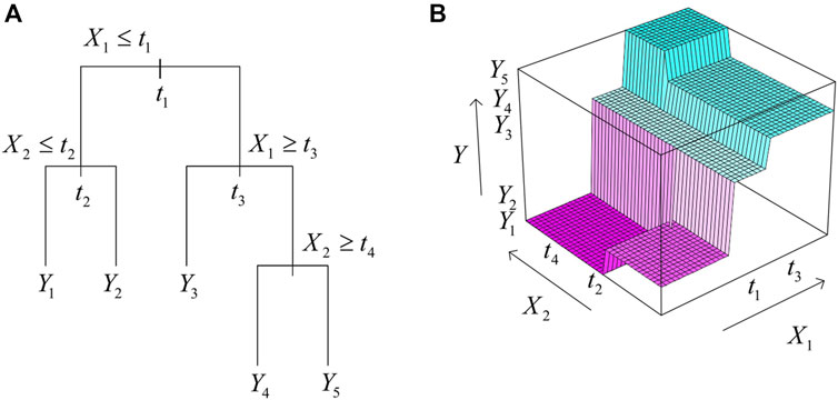
FIGURE 4. (A) shows a single regression tree with a response Y, in which X₁ and X₂ are two predictor variables, and t₁, t₂, etc. are split points. (B) shows the regression tree’s prediction surface. Source: Adapted from (Hastie et al., 2009, p. 306).

3.2.1.2 Boosting the Regression Tree—Boosted Regression Tree

Boosting is a technique that integrates the weak learners output (regression trees) to provide a stronger and amended predictive overall performance. Wherefore, the definitive model (BRT) would be a combination of several individual regression trees, fitted in a forward step-wise approach (Elith et al., 2008).

An efficient design for fitting a single decision tree is to grow a bigger tree. Afterward, one can prune it by collapsing the weakest links identified through cross-validation (Hastie et al., 2009).

Boosting is a numerical development approach to lessen the loss function through adding a new tree in each step that substantially lessens the loss function. The initial regression tree in BRT maximally lessens the loss function for the chosen tree size. Then, for every next step, the concentration is on the residuals: on variance in the response that the model has still not illustrated. The mean squared error (MSE) is a measure of the goodness of suitability. It computes the squared distance among an estimator and the anticipated parameter, which is given by:

$L\left(\theta \right)={\sum }_i{\left(y_i-{\widehat{y}}_i\right)}^2,(1)$

where L is the training loss function, θ is the parameters, and y is the prediction made from the training data (input X); $\widehat{y}$ is the prediction given by

${\widehat{y}}_i={\sum }_j{\theta }_j{X}_{ij}.(2)$

In boosting, models are fitted iteratively to the training records, gradually utilizing proper techniques to emphasize the observations modeled badly by using the current series of trees. Boosting algorithms differ in quantifying the shortage of suitability and deciding on the settings for the following repetition.

The BRT method has four essential features that have been applied in this study. They are:

1. The process is random (it contains a probabilistic or random factor). This random process enhances the predictive performance and lessens the variance of the definitive model, utilizing just a random subset of records to every new suitable tree (Friedman, 2002). This means that if a random seed is not set initially, the final models will be totally different at each run.

2. The consecutive model-fitting procedure builds on pre-fitted trees and concentrates more and more on predicting the most challenging observations. This differentiates the operation from one where a big tree is fitted to the data-series. Even so, if the ideal match was one tree, it might possibly be fitted through a sum of similar shrunken versions of itself in a boosted model.

3. Two critical parameters that are required to be set by the user:

a. Tree complexity (TC): this parameter specifies the split number in each tree. A TC value of 1 produces trees with just one split, meaning that the version ignores interactions among environmental variables. A TC value of 2 produces two splits and so forth.

b. Learning rate (LR—also known as the shrinkage parameter): A number between 0 and 1 identifies the rate that the algorithm has to converge and defines the contribution of every tree to the growth model. LR is inversely related to the number of repetitions needed for the algorithm to complete; since the value of LR is slight, numerous trees are created.

Together, these two parameters TC and LR define the number of trees needed for an optimum prediction. The aim is to find the combination of parameters that lead to the minimal error for the predictions. As a general rule, it is advisable to utilize a collection of tree complexity and learning rate values that produces a model containing a minimum of 1,000 trees. The optimum “TC” and “LR” values are contingent on the magnitude of the dataset, e.g., for datasets with less than 500 occurrence points (or epochs, as it is the case in this study). It is preferable to design simple trees (“TC” = 2 or 3) with learning rates sufficiently small to allow the model to reach the minimum of 1,000 trees.

4. Prediction from the BRT technique is simple; however, interpretation needs tools to identify which interactions and variables are important, and to visualize fitted functions (Elith et al., 2008).

The prediction in this study was achieved using the following predictors: precipitation (P), surface temperature (SMTL1), soil temperature (level 2/3/4) (SMTL2, SMTL3, SMTL4), surface air pressure (SP), soil moisture (SM), 2-meter temperature (T2m), instantaneous moisture flux (IE), and climate indices (CI). Figure 2 shows the correlation among them as well as with TWSA.

One of the BRT algorithm advantages is the easiness with which the influence of the predictors may be evaluated and largely disregards uninformative predictors while preparing trees.

Regularization is necessary for BRT due to its sequential model fitting, which lets trees to be added till the data are completely overfitted. This overfitting results in a poor performance on accurate data. BRT regularization includes the LR, optimization of tree number (NT), and TC altogether. The aim is to find the combination of parameters (LR, NT, and TC) that performs the minimal predictive error. BRT’s regularization and shrinkage are done using the Lasso method (most minor absolute shrinkage and selection operator). The Lasso method shrinks several coefficients and fixes others to 0, and it attempts to keep the good features of both subset selection and ridge regression.

3.2.2 Non-linear Autoregressive Neural Network With Exogenous Inputs—NARX

In this study, we used the NARX in the network design. NARX is an artificial neural network that also includes repetitive feedback from many network layers to the input layer (Ardalani-Farsa and Zolfaghari, 2010). Many researchers have vastly utilized it to model non-linear prediction processes (Ahmed et al., 2019; Ferreira et al., 2019). The NARX architecture predicts a signal via regressing the initial output signal values and the initial values of an independent (exogenous) input signal.

In this study, the NARX reconstruction model utilized 18 hidden layers. (Hereafter, NARX will be addressed simply as ANN.) These layers were adjusted by using a Bayesian regularization back propagation learning rule. The sigmoid transfer function was also utilized. The independent inputs consist of the same predictors that were used in BRT. After preparing the needed exogenous variables, the network was trained using the training period from April 2002 to November 2014. In the network designing, 70% of the data were used for training the network, 10% to validate and stop the training prior to overfitting, and 20% for testing (utilized as independent data). We trained the network with an open loop. After training and testing the network, the outputs from the ANN were validated using the metrics shown in Section 3.2.3. After that, the trained network was used to reconstruct the GRACE–TWSA from March 2002 to January 1982.

3.2.3 Assessment and Performance Measures

To assess the reliability of the BRT, and due to the lack of GRACE–TWSA, the reconstruction process was also validated via creating an akin network to predict TWSA from GLDAS–VIC, which is talented with a long-period time-series (1948–2015). This network was trained to predict GLDAS–VIC–TWSA (GLDAS–TWSA_BRT) from April 2002 to November 2014, after that, the trained network was utilized to backcast TWSA from March 2002 to January 1982. The reconstructed GLDAS–VIC time series from (March 2002 to January 1982) and the authentic datasets were utilized to validate the outputs from the BRT.

Likewise, to assess the reliability of ANN in reconstructing the long-period TWSA, GLDAS–VIC was utilized in a “closed-loop” simulation to evaluate the goodness of the extended TWSA series from March 2002 to January 1982. The networks were trained with the same predictors (exogenous variables) as those of GRACE–TWSA (Figure 3) for the same duration (April 2002 to November 2014). Afterward, the network was used to predict GLDAS–VIC TWSA (GLDAS-TWSA_ANN) from January 1982 to March 2002, and the outcomes were compared to the original GLDAS–VIC TWSA dataset. The same process was repeated for BRT reconstruction.

The performance of the reconstructed TWSA series was determined using the Nash–Sutcliffe efficiency (NSE) coefficient, and the root-mean-square error (RMSE) given as (e.g., Moriasi et al., 2007):

$\text{NSE}=1-\frac{{\sum }_{i=1}^t{\left(\text{TWS}{\text{A}}_{\text{obs},i}-\text{TWS}{\text{A}}_{\text{rec},i}\right)}^2}{{\sum }_{i=1}^t{\left(\text{TWS}{\text{A}}_{\text{obs},i}-{\overline{\text{TWSA}}}_{\text{obs}}\right)}^2},(3)$

and

$\text{RMSE}=\sqrt{\frac{1}{t}\sum _{i=1}^t{\left(\text{TWS}{\text{A}}_{\text{obs},i}-\text{TWS}{\text{A}}_{\text{rec},i}\right)}^2},(4)$

respectively.

The Pearson’s correlation coefficient (PCC), given as:

$\text{PCC}=\frac{{\sum }_{i=1}^t\left(\text{TWS}{\text{A}}_{\text{rec},i}-\text{TWS}{\text{A}}_{\text{rec}}\right)\left(\text{TWS}{\text{A}}_{\text{obs},i}-{\overline{\text{TWSA}}}_{\text{obs}}\right)}{\sqrt{{\sum }_{i=1}^t{\left(\text{TWS}{\text{A}}_{\text{rec},i}-\text{TWS}{\text{A}}_{\text{rec}}\right)}^2}\sqrt{{\sum }_{i=1}^t{\left(\text{TWS}{\text{A}}_{\text{obs},i}-{\overline{\text{TWSA}}}_{\text{obs}}\right)}^2}},(5)$

was used to describe the degree of collinearity between the simulated and observed data.

In Eqs 3–5, the variables are as follow: t represents the length of the time series of TWSA (that is, the total number of months considered in the evaluation), TWSA_rec is the resulting reconstructed TWSA series based on BRT or ANN, TWSA_obs is the observed TWSA based on GRACE data, and ${\overline{\text{TWSA}}}_{\text{obs}}$ is the mean value of the observed TWSA series.

4 Results

4.1 Terrestrial Water Storage Anomaly’s Reconstruction Using the Boosted Regression Tree and Artificial Neural Network

We partitioned the data into training and testing sets using 80% of the data randomly assigned to the training set, and 20% of the data randomly assigned as the testing set (we got the best results with this partitioning percentage). After several trial attempts to find the appropriate values of the parameters to obtain an optimal accuracy of the TWSA prediction, it was found that the TC = 5 and LR = 0.0035 with 2,000 trees provided the best results over the YRB. The number of trees after the regularization and shrinkage was 200. Figures 5A,C show the fitting against training and testing data for TWSA, respectively. Hence, inspecting the reconstructed values from the testing step, we found an overall agreement with the actual values of the TWSA series for the specific months (Figure 5C). The deviation residuals are used as a loss function to assess the reconstruction, which in terms of RMSE has a value of 18.94 mm. Furthermore, the NSE coefficient based on the comparison between the actual and reconstructed TWSA series in the testing step (Figure 5C) presents a value of approximately 0.89 and a PCC of 0.95 (Table 1).

FIGURE 5

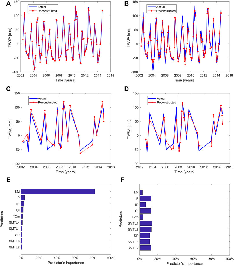
FIGURE 5. (A,B) show the training stage of the prediction of the TWSA series for the YRB based on BRT and ANN, respectively. (C,D) show the test stage of the TWSA series of the YRB based on BRT and ANN, respectively. (E,F) show the predictors’ importance in both BRT and ANN methods, respectively.

TABLE 1

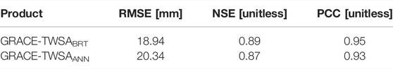
TABLE 1. Summary statistics for the reconstructed GRACE–TWSA based on BRT and ANN during the validation stage using 20% of the whole time series.

Likewise, the ANN was used in this study to reconstruct GRACE–TWSA backward from March 2002 to January 1982 precisely in the same way as BRT. In an open loop, the network was trained and tested from April 2002 to November 2014. The optimal ANN model used to backcast GRACE–TWSA over the YRB was chosen from all possible combinations of neurons and delays. Figures 5B, D show the time-series response during the training and the test stages, respectively. Upon training and testing the network, the results show that the accuracy of the network in terms of RMSE value is 20.34 mm (Table 1). This shows an underperformance of the ANN-reconstructed series of about 6.9% in terms of the BRT-based reconstruction. Furthermore, the NSE presents a value of approximately 0.87, and the PCC shows a value of 0.93 (Table 1), slightly lower than those based on the BRT evaluation (Table 1).

The relative importance of the predictors used in the BRT model shows that soil moisture (SM) is the most important variable in TWSA reconstruction over the YRB showing a relative contribution of about 81.9%. Conversely, soil temperature level 2 (SMTL2) has the lowest importance, with a contribution of about 1.0%. Likewise, Figure 5F indicates the relative importance of the input variables (predictor importance) of the predictors used in the ANN model. It can be seen that most of the variables present relative contributions between 11% and 14% (Figure 5F). SM usually shows a significantly positive correlation with variations of regional TWSA (Figure 2). However, SM presents the lowest contribution with a relative weight of 3.1% for the overall reconstruction of the TWSA series over YRB; the same holds for the instantaneous moisture flux (IE), 6.8%, and T2m, 3.9%. However, ANN models may be complicated, and deciding which predictor is more valuable can be difficult without further experiments, which is beyond the scope of the present work.

The reconstructed TWSA time-series covering the 32 years from January 1982 to December 2014 based on the respective training for BRT and ANN as described previously were undertaken (Figure 6). The missing values are seen in the original GRACE–TWSA series (Figure 6) and were also provisioned in the reconstruction. The overall behaviors of the maximum and minimum amplitudes over the backcasted period (January 1982 to March 2002) are consistent with the observed data period (actual) covering the period from April 2002 to December 2014. As already mentioned and presented in Figures 5A, C, the overall match between reconstructed and the actual TWSA series is seen for BRT-based results (Figure 6). Generally, ANN-based results overestimate the high (e.g., early 2014) and low amplitudes (e.g., middle 2004). Its high RMSE value of 20.34 mm confirms these discrepancies compared to BRT (18.94 mm) from April 2002 to December 2014 (Table 1).

FIGURE 6

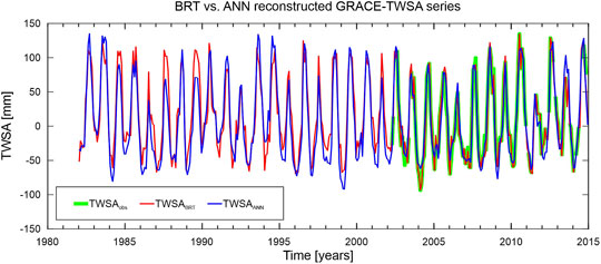
FIGURE 6. Time series of TWSA predicted by the BRT and ANN (1982–2014) and those observed (April 2002–December 2014).

Likewise, from January 1982 to March 2002, the ANN-reconstructed TWSA series generally presented amplitudes higher than those based on the BRT algorithm. Nevertheless, the BRT-reconstructed TWSA series showed higher amplitudes; for example, in the middle 1987 and 1989 periods. Notably, the lower amplitudes of TWSA are from 1990 to 1994, which could be associated with a mild drought during this period. Nevertheless, whatever could be the use and application of the GRACE–TWSA reconstructed time-series (Figure 6), assessing the algorithms are still necessary since there is no observed TWSA over the backcasted period (1982–2001). Hence, a simulation is presented in the following (Section 4.2) to address such a question.

4.2 Assessment of the Boosted Regression Tree and Artificial Neural Network for Reconstructing the Terrestrial Water Storage Anomaly—A “Closed-Loop” Simulation

The aim of this experiment was two-fold: 1) to evaluate the performance of the BRT and ANN, and 2) to assess the reliability of the reconstructed series over the period of 1982–2002.

A simulation of TWSA was implemented within a closed-loop process to estimate the goodness of the reconstructed TWSA series from 2002 to 1982. The simulations of TWSA are based on the water-storage compartments available in GLDAS–VIC covering the period from January 1982 to December 2014 (Section 3.1). The GLDAS–VIC-simulated TWSA series was split into two parts: one from April 2002 to November 2014, just like the GRACE datasets, and another from January 1982 to March 2002 (the period to be reconstructed). The latter is used only for assessment purposes.

First, BRT reconstruction was carried out using the same predictors as described in Section 3.1, with the only difference being the replacement of GRACE–TWSA (April 2002–November 2014) by the GLDAS–VIC–TWSA (April 2002–November 2014). All the predictors were not taken from GLDAS–VIC, thereby being an independent evaluation. Second, as with BRT, the reconstruction using the ANN–NARX based on GLDAS–VIC–TWSA was also carried out. Figure 7 shows the reconstructed TWSA time-series based on BRT and ANN (GLDAS–TWSA_BRT and GLDAS–TWSA_ANN) as well as the original GLDAS–TWSA series (GLDAS–TWSA_obs).

FIGURE 7

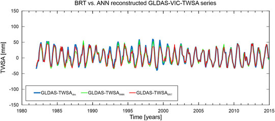
FIGURE 7. Reconstructed time series of GLDAS–TWSA; the blue line is the original GLDAS–TWSA time series (observation), the red line is the GLDAS–TWSA time series as estimated by BRT, and the green line is the GLDAS–TWSA time series as estimated by ANN.

The overall behaviors of the maximum and minimum amplitudes over the backcasted period (1982–2001) by the BRT method (GLDAS–TWSA_BRT) are more consistent with the observed data amplitudes (GLDAS–TWSA_obs) in comparison with those amplitudes based on ANN (GLDAS–TWSA_ANN, see Figure 7). Specifically, the GLDAS–TWSA_ANN series generally underestimate the maximum peaks, whereas the low peaks seem to agree with those based on BRT and the observed values.

In the assessment process and during the training and testing stages using GLDAS–VIC–TWSA over the period from April 2002 to November 2014, the BRT network performance presents an RMSE value of 5.68 mm, NSE value of 0.94, and PCC value of 0.97 (Table 2). Furthermore, applying ANN to predict GLDAS–VIC–TWSA over the period April 2002 to November 2014, the performance of ANN presents an RMSE value of 5.72 mm, NSE value of 0.94, and the PCC of 0.97 (Table 2). A marginal improvement in terms of RMSE of approximately 0.7% was found for BRT for the testing stage.

TABLE 2

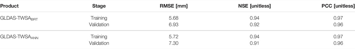
TABLE 2. Summary statistics for the reconstructed GLDAS–VIC–TWSA based on BRT and ANN during the training stage and validation. The validation refers to the comparison between the reconstructed series and those observed in Figure 7, that is, the closed-loop simulation.

Nevertheless, a validation to assess the reliability of BRT and ANN algorithms to reconstruct GLDAS–VIC–TWSA over the period January 1982–March 2002 was carried out. Contrary to what was done with GRACE–TWSA, the GLDAS–VIC–TWSA series can be used to validate the reconstructed values since they are available over the desired period. Overall, the results of the BRT indicate more reliability with a performance better than ANN with an RMSE value of 6.93 mm, NSE value of 0.92, and PCC value of 0.96 (Table 2). At the same time, the results of ANN present a value of RMSE of 7.30 mm, NSE of 0.91, and PCC of 0.96 (Table 2).

5 Discussion

Predictions gained from modeling and simulations are now considered an important goal of environmental studies, as they underpin important decisions by hydrologists and engineers, which can help inform on policy. With this in mind, the principal focus of this study was to reconstruct the actual time series of GRACE–TWSA backward from 2014 to 1982 (32 years). The reconstruction of the GRACE-derived TWSA over the YRB used BRT and ANN (represented by NARX) algorithms. Consequently, the contributions of the present work are 1) validating the BRT algorithm, given that errors are within a tolerable range such as the GRACE uncertainty range, and 2) providing an extended time-series that support studies such as droughts. Although several studies have considered the potential of TWSA reconstruction over the YRB (e.g., Zhang et al., 2016), none has considered the use of BRT to reconstruct TWSA.

First, BRT was used to reconstruct GRACE–TWSA over the YRB, where 80% of the data were utilized for training, whereas the remaining 20% of the data were utilized for testing the network. Notably, this partitioning of data was selected after several trials to get the best accuracy. The model was constructed based on its physical relationships with ten hydro-climatic variables (the predictors). These variables are: precipitation (P), surface temperature (SMTL1), soil temperature (level 2/3/4) (SMTL2, SMTL3, SMTL4), surface air pressure (SP), soil moisture (SM), 2-meter temperature (T2m), instantaneous moisture flux (IE), and climate indices (CI). This network’s results showed an RMSE value of 18.94 mm, NSE value of 0.89, and PCC value of 0.95. This shows the consistency of the reconstructed (predicted) and the observed (actual) TWSA series (Figures 5A,C). Second, ANN was trained precisely in the same way as BRT, in which the performance of the series indicated a slight underperformance of about 7.4%, 2.2%, and 2.1%, respectively, in terms of RMSE, NSE, and PCC (cf. Table 1). Both methods present RMSE values within GRACE’s overall accuracy of about 20–30 mm over most river basins (Scanlon et al., 2016). Although the data used in this study were of coarse spatial resolution (1°-by-1°), they were valuable to prove the effectiveness of both algorithms for prediction with an acceptable accuracy.

Because the BRT technique is insensitive to multi-collinearity and outliers, it can fit complicated non-linear relationships, and it can automatically deal with the interactive impacts among predictors (Elith et al., 2006; Elith et al., 2008; Dedman et al., 2017). Hitherto, BRT seems a highly feasible technique to reconstruct TWSA using only one predictor like soil moisture (Figure 5E), and that is reasonable because SM is very similar and highly correlated with TWSA in the YRB (see Figure 2, and also cf. Ferreira et al., 2020a). This result also aligns with the finds of Naghibi and Pourghasemi (2015). They found that BRT used only eight variables selected from the original data (14 variables). Some authors also declared that a close model would be more steady and easier to generalize (Catry et al., 2009; Vilar et al., 2010). Conversely, ANN-based reconstruction seems to necessitate more predictors. It used all predictors to achieve the prediction process and showed that SM got the lowest contribution in the TWSA prediction (Figure 5F). This seems to be an obvious advantage of BRT compared to ANN. One could rely upon only one of the most accurate datasets (e.g., precipitation) based on remotely sensed or in-situ measurements to reconstruct TWSA instead of using all potential predictors (compare Figures 5E,F).

Finally, based on BRT and ANN, the GRACE–TWSA was backcasted from December 2014 to January 1982 (Figure 6). However, an important question regarding the suitability of the extended GRACE–TWSA series is how reliable are GRACE–TWSA reconstructed series (Figure 6)? In the absence of the observed TWSA between January 1982 and March 2002, a closed-loop simulation using TWSA from GLDAS–VIC to evaluate the reliability of BRT and ANN was considered. A period equivalent to the GRACE data (April 2002–November 2014) was used to generate BRT and ANN and then reconstruct the GLDAS–VIC TWSA till 1982 (Figure 7). Both networks were trained to simulate GLDAS–VIC TWSA based on their non-linear physical relationships with the ten hydro-climatic variables. The BRT results showed a slightly better accuracy than those based on ANN (Table 2). Overall, BRT and ANN showed excellent performances with RMSE values of 6.93 and 7.30 mm, respectively. This finding aligns with those from previous studies (e.g., Pourghasemi and Rahmati, 2018), which proved that BRT has a better performance than ANN. Additionally, some studies evaluated several different machine-learning techniques and found that BRT performed better than other popular algorithms (see, e.g., Cunningham et al., 2011; Naghibi and Pourghasemi, 2015; Nolan et al., 2015; Naghibi et al., 2016, for an exhaustive comparison of BRT with other algorithms applied to different subjects). Considering the ratio between the RMSE of the reconstructed GRACE–TWSA with those from GLDAS–VIC–TWSA during the training phases (Tables 1, 2) for the respective algorithms (BRT and ANN), it is possible to derive scale factors to infer the respective RMSEs of GRACE–TWSA of 23.10 and 25.96 mm, respectively. Again, such accuracies are akin to that of the GRACE era TWSA. Hence, this indicates that the temporal series shown in Figure 6 can be used in hydrological studies such as hydrological drought characterizations and the assessment of long-term changes of TWSA. This could be the subject of a separate study.

6 Conclusion

In the case of long-term studies (e.g., drought and flood assessments), TWSA from GRACE and GRACE-FO missions cover a relatively short period of approximately 20 years. This means that it cannot be effectively applied for impact assessments from droughts and floods, and deduce long-term water availability over the YRB. To address this limitation, this study compared two machine-learning approaches over the YRB to predict and reconstruct the TWSA back to 1982. To this end, boosted regression tree (BRT), a popular machine learning algorithm that increases the model’s accuracy, was used to reconstruct GRACE–TWSA. BRT is a robust algorithm that works very well with large datasets or when there are many hydro-climatic variables compared to the number of observations. They are also very robust in circumventing problems associated with missing values and outliers. This study found that BRT and artificial neural network (ANN, represented by a non-linear-autoregressive neural network with exogenous inputs—NARX) methods appeared robust enough to sufficiently reconstruct GRACE–TWSA over the YRB with accuracy akin to the GRACE dataset. The validation results of both techniques indicated that the BRT technique is a more reliable and “economic” model to reconstruct TWSA over the YRB. That is, the most correlated predictors, in our case, soil moisture and precipitation, could be enough to reconstruct the TWSA time-series. Hence, the method is highly recommended for study areas where only a few datasets are available as predictive variables (e.g., soil moisture and/or precipitation).

Data Availability Statement

Publicly available datasets were analyzed in this study. These data can be found here: GPCC precipitation available by Deutscher Wetterdienst at https://opendata.dwd.de/climate_environment/GPCC/html/download_gate.html; ERA Interim datasets are available by the ECMWF at https://apps.ecmwf.int/datasets/data/interim-full-moda/levtype=sfc/; GLDAS fields are available by The NASA Goddard Earth Sciences Data and Information Services Center (GES DISC) at https://ldas.gsfc.nasa.gov/gldas/gldas-get-data; the climate indices was retrieved from the NOAA Physical Sciences Laboratory (PSL) through the link https://psl.noaa.gov/data/climateindices/list/; and the GRACE-TWSA monthly grids are available at https://grace.jpl.nasa.gov/data/get-data/.

Author Contributions

RD and VF conceived and designed the experiment. RD processed the datasets. CN and FC edited the final version of the manuscript. RD and BY wrote the original draft, and all authors contributed to writing the manuscript.

Funding

This study was supported by the National Key R&D Program (grant no. 2018YFA0605402).

Conflict of Interest

The authors declare that the research was conducted in the absence of any commercial or financial relationships that could be construed as a potential conflict of interest.

Publisher’s Note

All claims expressed in this article are solely those of the authors and do not necessarily represent those of their affiliated organizations, or those of the publisher, the editors, and the reviewers. Any product that may be evaluated in this article, or claim that may be made by its manufacturer, is not guaranteed or endorsed by the publisher.

Acknowledgments

The authors are grateful to all the dataset providers, as mentioned in Section 3.1, on which the analysis in this manuscript is based. Bin Yong acknowledges the support from China’s National Key R&D Program (grant no. 2018YFA0605402). Finally, we acknowledge the Associate Editor and two reviewers for their remarks which helped improve the quality of this manuscript.

References

Abeare, S. (2009). Comparisons of Boosted Regression Tree, GLM and GAM Performance in the Standardization of Yellowfin Tuna Catch-Rate Data from the Gulf of Mexico Lonline [sic] Fishery. Ph.D. Thesis. Baton Rouge: Louisiana State University.

Google Scholar

Ahmed, M., Sultan, M., Wahr, J., and Yan, E. (2014). The Use of GRACE Data to Monitor Natural and Anthropogenic Induced Variations in Water Availability across Africa. Earth Sci. Rev. 136, 289–300. doi:10.1016/j.earscirev.2014.05.009

CrossRef Full Text | Google Scholar

Ahmed, M., Sultan, M., Elbayoumi, T., and Tissot, P. (2019). Forecasting GRACE Data over the African Watersheds Using Artificial Neural Networks. Remote Sens. 11, 1769. doi:10.3390/rs11151769

CrossRef Full Text | Google Scholar

Ardalani-Farsa, M., and Zolfaghari, S. (2010). Chaotic Time Series Prediction with Residual Analysis Method Using Hybrid Elman-NARX Neural Networks. Neurocomputing 73, 2540–2553. doi:10.1016/j.neucom.2010.06.004

CrossRef Full Text | Google Scholar

Becker, M., Meyssignac, B., Xavier, L., Cazenave, A., Alkama, R., and Decharme, B. (2011). Past Terrestrial Water Storage (1980-2008) in the Amazon Basin Reconstructed from GRACE and In Situ River Gauging Data. Hydrol. Earth Syst. Sci. 15, 533–546. doi:10.5194/hess-15-533-2011

CrossRef Full Text | Google Scholar

Catry, F. X., Rego, F. C., Bação, F. L., and Moreira, F. (2009). Modeling and Mapping Wildfire Ignition Risk in Portugal. Int. J. Wildland Fire 18, 921–931. doi:10.1071/WF07123

CrossRef Full Text | Google Scholar

Chen, H., Zhang, W., Nie, N., and Guo, Y. (2019). Long-term Groundwater Storage Variations Estimated in the Songhua River Basin by Using GRACE Products, Land Surface Models, and In-Situ Observations. Sci. Total Environ. 649, 372–387. doi:10.1016/j.scitotenv.2018.08.352

PubMed Abstract | CrossRef Full Text | Google Scholar

Cunningham, S. C., Thomson, J. R., Mac Nally, R., Read, J., and Baker, P. J. (2011). Groundwater Change Forecasts Widespread Forest Dieback across an Extensive Floodplain System. Freshw. Biol. 56, 1494–1508. doi:10.1111/j.1365-2427.2011.02585.x

CrossRef Full Text | Google Scholar

de Linage, C., Famiglietti, J. S., and Randerson, J. T. (2014). Statistical Prediction of Terrestrial Water Storage Changes in the Amazon Basin Using Tropical Pacific and North Atlantic Sea Surface Temperature Anomalies. Hydrol. Earth Syst. Sci. 18, 2089–2102. doi:10.5194/hess-18-2089-2014

CrossRef Full Text | Google Scholar

Dedman, S., Officer, R., Clarke, M., Reid, D. G., and Brophy, D. (2017). Gbm.auto: A Software Tool to Simplify Spatial Modelling and Marine Protected Area Planning. PLOS ONE 12, e0188955–16. doi:10.1371/journal.pone.0188955

PubMed Abstract | CrossRef Full Text | Google Scholar

Dong, Q., Fang, D., Zuo, J., and Wang, Y. (2019). Hydrological Alteration of the Upper Yangtze River and its Possible Links with Large-Scale Climate Indices. Hydrol. Res. 50, 1120–1137. doi:10.2166/nh.2019.112

CrossRef Full Text | Google Scholar

Elith, J., Graham, C., Anderson, R. R., Dudík, M., Ferrier, S., Guisan, A., et al. (2006). Novel Methods Improve Prediction of Species' Distributions from Occurrence Data. Ecography 29, 129–151. doi:10.1111/j.2006.0906-7590.04596.x

CrossRef Full Text | Google Scholar

Elith, J., Leathwick, J. R., and Hastie, T. (2008). A Working Guide to Boosted Regression Trees. J. Anim. Ecol. 77, 802–813. doi:10.1111/j.1365-2656.2008.01390.x

PubMed Abstract | CrossRef Full Text | Google Scholar

Ferreira, V., Andam-Akorful, S., Dannouf, R., and Adu-Afari, E. (2019). A Multi-Sourced Data Retrodiction of Remotely Sensed Terrestrial Water Storage Changes for West Africa. Water 11, 401. doi:10.3390/w11020401

CrossRef Full Text | Google Scholar

Ferreira, V. G., Yong, B., Tourian, M. J., Ndehedehe, C. E., Shen, Z., Seitz, K., et al. (2020a). Characterization of the Hydro-Geological Regime of Yangtze River Basin Using Remotely-Sensed and Modeled Products. Sci. Total Environ. 718, 137354. doi:10.1016/j.scitotenv.2020.137354

PubMed Abstract | CrossRef Full Text | Google Scholar

Ferreira, V. G., Yong, B., Seitz, K., Heck, B., and Grombein, T. (2020b). Introducing an Improved GRACE Global Point-Mass Solution-A Case Study in Antarctica. Remote Sens. 12, 3197. doi:10.3390/rs12193197

CrossRef Full Text | Google Scholar

Forootan, E., Didova, O., Schumacher, M., Kusche, J., and Elsaka, B. (2014a). Comparisons of Atmospheric Mass Variations Derived from ECMWF Reanalysis and Operational Fields, over 2003-2011. J. Geod. 88, 503–514. doi:10.1007/s00190-014-0696-x

CrossRef Full Text | Google Scholar

Forootan, E., Kusche, J., Loth, I., Schuh, W.-D., Eicker, A., Awange, J., et al. (2014b). Multivariate Prediction of Total Water Storage Changes over West Africa from Multi-Satellite Data. Surv. Geophys. 35, 913–940. doi:10.1007/s10712-014-9292-0

CrossRef Full Text | Google Scholar

Friedman, J., Tibshirani, R., and Hastie, T. (2000). Additive Logistic Regression: A Statistical View of Boosting (With Discussion and a Rejoinder by the Authors). Ann. Stat. 28, 337–407. doi:10.1214/aos/1016218223

CrossRef Full Text | Google Scholar

Friedman, J. H. (2002). Stochastic Gradient Boosting. Comput. Stat. Data Analysis 38, 367–378. doi:10.1016/S0167-9473(01)00065-2

CrossRef Full Text | Google Scholar

Hastie, T., Tibshirani, R., and Friedman, J. (2009). The Elements of Statistical Learning. Springer Series in Statistics. New York, NY: Springer New York. doi:10.1007/978-0-387-84858-7

CrossRef Full Text | Google Scholar

Landerer, F. W., and Swenson, S. C. (2012). Accuracy of Scaled GRACE Terrestrial Water Storage Estimates. Water Resour. Res. 48, W04531. doi:10.1029/2011WR011453

CrossRef Full Text | Google Scholar

Leathwick, J., Elith, J., Francis, M., Hastie, T., and Taylor, P. (2006). Variation in Demersal Fish Species Richness in the Oceans Surrounding New Zealand: An Analysis Using Boosted Regression Trees. Mar. Ecol. Prog. Ser. 321, 267–281. doi:10.3354/meps321267

CrossRef Full Text | Google Scholar

Leathwick, J. R., Elith, J., Chadderton, W. L., Rowe, D., and Hastie, T. (2008). Dispersal, Disturbance and the Contrasting Biogeographies of New Zealand's Diadromous and Non-diadromous Fish Species. J. Biogeogr. 35, 1481–1497. doi:10.1111/j.1365-2699.2008.01887.x

CrossRef Full Text | Google Scholar

Li, F., Kusche, J., Chao, N., Wang, Z., and Löcher, A. (2021). Long-term (1979-present) Total Water Storage Anomalies over the Global Land Derived by Reconstructing GRACE Data. Geophys. Res. Lett. 48, e2021GL093492. doi:10.1029/2021GL093492

CrossRef Full Text | Google Scholar

Long, D., Shen, Y., Sun, A., Hong, Y., Longuevergne, L., Yang, Y., et al. (2014). Drought and Flood Monitoring for a Large Karst Plateau in Southwest China Using Extended GRACE Data. Remote Sens. Environ. 155, 145–160. doi:10.1016/j.rse.2014.08.006

CrossRef Full Text | Google Scholar

Long, D., Yang, Y., Wada, Y., Hong, Y., Liang, W., Chen, Y., et al. (2015). Deriving Scaling Factors Using a Global Hydrological Model to Restore GRACE Total Water Storage Changes for China's Yangtze River Basin. Remote Sens. Environ. 168, 177–193. doi:10.1016/j.rse.2015.07.003

CrossRef Full Text | Google Scholar

Long, D., Chen, X., Scanlon, B. R., Wada, Y., Hong, Y., Singh, V. P., et al. (2016). Have Grace Satellites Overestimated Groundwater Depletion in the Northwest India Aquifer? Sci. Rep. 6, 24398. doi:10.1038/srep24398

PubMed Abstract | CrossRef Full Text | Google Scholar

Ma, S., Wu, Q., Wang, J., and Zhang, S. (2017). Temporal Evolution of Regional Drought Detected from GRACE TWSA and CCI SM in Yunnan Province, China. Remote Sens. 9, 1124. doi:10.3390/rs9111124

CrossRef Full Text | Google Scholar

Mo, X., Wu, J. J., Wang, Q., and Zhou, H. (2016). Variations in Water Storage in China over Recent Decades from GRACE Observations and GLDAS. Nat. Hazards Earth Syst. Sci. 16, 469–482. doi:10.5194/nhess-16-469-2016

CrossRef Full Text | Google Scholar

Moriasi, D. N., Arnold, J. G., Van Liew, M. W., Bingner, R. L., Harmel, R. D., and Veith, T. L. (2007). Model Evaluation Guidelines for Systematic Quantification of Accuracy in Watershed Simulations. Trans. ASABE 50, 885–900. doi:10.13031/2013.23153

CrossRef Full Text | Google Scholar

Mukherjee, A., and Ramachandran, P. (2018). Prediction of GWL with the Help of GRACE TWS for Unevenly Spaced Time Series Data in India : Analysis of Comparative Performances of SVR, ANN and LRM. J. Hydrol. 558, 647–658. doi:10.1016/j.jhydrol.2018.02.005

CrossRef Full Text | Google Scholar

Mukhopadhyay, A. (2003). Application of Visual, Statistical and Artificial Neural Network Methods in the Differentiation of Water from the Exploited Aquifers in Kuwait. Hydrogeol. J. 11, 343–356. doi:10.1007/s10040-003-0257-5

CrossRef Full Text | Google Scholar

Naghibi, S. A., and Pourghasemi, H. R. (2015). A Comparative Assessment between Three Machine Learning Models and Their Performance Comparison by Bivariate and Multivariate Statistical Methods in Groundwater Potential Mapping. Water Resour. Manage 29, 5217–5236. doi:10.1007/s11269-015-1114-8

CrossRef Full Text | Google Scholar

Naghibi, S. A., Pourghasemi, H. R., and Dixon, B. (2016). GIS-based Groundwater Potential Mapping Using Boosted Regression Tree, Classification and Regression Tree, and Random Forest Machine Learning Models in Iran. Environ. Monit. Assess. 188, 44. doi:10.1007/s10661-015-5049-6

PubMed Abstract | CrossRef Full Text | Google Scholar

Ndehedehe, C. E., and Ferreira, V. G. (2020). Assessing Land Water Storage Dynamics over South America. J. Hydrol. 580, 124339. doi:10.1016/j.jhydrol.2019.124339

CrossRef Full Text | Google Scholar

Nolan, B. T., Fienen, M. N., and Lorenz, D. L. (2015). A Statistical Learning Framework for Groundwater Nitrate Models of the Central Valley, California, USA. J. Hydrology 531, 902–911. doi:10.1016/j.jhydrol.2015.10.025

CrossRef Full Text | Google Scholar

Pourghasemi, H. R., and Rahmati, O. (2018). Prediction of the Landslide Susceptibility: Which Algorithm, Which Precision? CATENA 162, 177–192. doi:10.1016/j.catena.2017.11.022

CrossRef Full Text | Google Scholar

Rahman, A. T. M. S., Hosono, T., Quilty, J. M., Das, J., and Basak, A. (2020). Multiscale Groundwater Level Forecasting: Coupling New Machine Learning Approaches with Wavelet Transforms. Adv. Water Resour. 141, 103595. doi:10.1016/j.advwatres.2020.103595

CrossRef Full Text | Google Scholar

Reager, J. T., Thomas, B. F., and Famiglietti, J. S. (2014). River Basin Flood Potential Inferred Using GRACE Gravity Observations at Several Months Lead Time. Nat. Geosci. 7, 588–592. doi:10.1038/ngeo2203

CrossRef Full Text | Google Scholar

Rodell, M., Famiglietti, J. S., Chen, J., Seneviratne, S. I., Viterbo, P., Holl, S., et al. (2004a). Basin Scale Estimates of Evapotranspiration Using GRACE and Other Observations. Geophys. Res. Lett. 31, L20504. doi:10.1029/2004GL020873

CrossRef Full Text | Google Scholar

Rodell, M., Houser, P. R., Jambor, U., Gottschalck, J., Mitchell, K., Meng, C.-J., et al. (2004b). The Global Land Data Assimilation System. Bull. Amer. Meteor. Soc. 85, 381–394. doi:10.1175/BAMS-85-3-381

CrossRef Full Text | Google Scholar

Rodell, M., Velicogna, I., and Famiglietti, J. S. (2009). Satellite-based Estimates of Groundwater Depletion in India. Nature 460, 999–1002. doi:10.1038/nature08238

PubMed Abstract | CrossRef Full Text | Google Scholar

Rodell, M., Famiglietti, J. S., Wiese, D. N., Reager, J. T., Beaudoing, H. K., Landerer, F. W., et al. (2018). Emerging Trends in Global Freshwater Availability. Nature 557, 651–659. doi:10.1038/s41586-018-0123-1

PubMed Abstract | CrossRef Full Text | Google Scholar

Scanlon, B. R., Zhang, Z., Save, H., Wiese, D. N., Landerer, F. W., Long, D., et al. (2016). Global Evaluation of New GRACE Mascon Products for Hydrologic Applications. Water Resour. Res. 52, 9412–9429. doi:10.1002/2016WR019494

CrossRef Full Text | Google Scholar

Schapire, R. E. (2003). The Boosting Approach to Machine Learning: An Overview. New York, NY: Springer, 149–171. chap. 9. doi:10.1007/978-0-387-21579-2_9

CrossRef Full Text | Google Scholar

Schneider, U., Becker, A., Finger, P., Meyer-Christoffer, A., Ziese, M., and Rudolf, B. (2013). GPCC's New Land Surface Precipitation Climatology Based on Quality-Controlled In Situ Data and its Role in Quantifying the Global Water Cycle. Theor. Appl. Climatol. 115, 15–40. doi:10.1007/s00704-013-0860-x

CrossRef Full Text | Google Scholar

Sharafati, A., Asadollah, S. B. H. S., and Neshat, A. (2020). A New Artificial Intelligence Strategy for Predicting the Groundwater Level over the Rafsanjan Aquifer in Iran. J. Hydrol. 591, 125468. doi:10.1016/j.jhydrol.2020.125468

CrossRef Full Text | Google Scholar

Smith, C. A., and Sardeshmukh, P. D. (2000). The Effect of ENSO on the Intraseasonal Variance of Surface Temperatures in Winter. Int. J. Climatol. 20, 1543–1557. doi:10.1002/1097-0088(20001115)20:13<1543::AID-JOC579>3.0.CO;2-A

CrossRef Full Text | Google Scholar

Sun, Z., Zhu, X., Pan, Y., Zhang, J., and Liu, X. (2018). Drought Evaluation Using the GRACE Terrestrial Water Storage Deficit over the Yangtze River Basin, China. Sci. Total Environ. 634, 727–738. doi:10.1016/j.scitotenv.2018.03.292

PubMed Abstract | CrossRef Full Text | Google Scholar

Syed, T. H., Famiglietti, J. S., Chen, J., Rodell, M., Seneviratne, S. I., Viterbo, P., et al. (2005). Total Basin Discharge for the Amazon and Mississippi River Basins from GRACE and a Land-Atmosphere Water Balance. Geophys. Res. Lett. 32, L24404. doi:10.1029/2005GL024851

CrossRef Full Text | Google Scholar

Velicogna, I., Tong, J., Zhang, T., and Kimball, J. S. (2012). Increasing Subsurface Water Storage in Discontinuous Permafrost Areas of the Lena River Basin, Eurasia, Detected from GRACE. Geophys. Res. Lett. 39, 1–5. doi:10.1029/2012GL051623

CrossRef Full Text | Google Scholar

Vilar, L., Woolford, D. G., Martell, D. L., and Martín, M. P. (2010). A Model for Predicting Human-Caused Wildfire Occurrence in the Region of Madrid, Spain. Int. J. Wildland Fire 19, 325–337. doi:10.1071/WF09030

CrossRef Full Text | Google Scholar

Vishwakarma, B. D. (2020). Monitoring Droughts from GRACE. Front. Environ. Sci. 8, 1–6. doi:10.3389/fenvs.2020.584690

CrossRef Full Text | Google Scholar

Wang, F., Chen, Y., Li, Z., Fang, G., Li, Y., Wang, X., et al. (2021). Developing a Long Short-Term Memory (LSTM)-based Model for Reconstructing Terrestrial Water Storage Variations from 1982 to 2016 in the Tarim River Basin, Northwest China. Remote Sens. 13, 889–918. doi:10.3390/rs13050889

CrossRef Full Text | Google Scholar

Wilby, R. L., Abrahart, R. J., and Dawson, C. W. (2003). Detection of Conceptual Model Rainfall-Runoff Processes inside an Artificial Neural Network. Hydrol. Sci. J. 48, 163–181. doi:10.1623/hysj.48.2.163.44699

CrossRef Full Text | Google Scholar

Yin, W., Hu, L., Han, S.-c., Zhang, M., and Teng, Y. (2019). Reconstructing Terrestrial Water Storage Variations from 1980 to 2015 in the Beishan Area of China. Geofluids 2019, 1–13. doi:10.1155/2019/3874742

CrossRef Full Text | Google Scholar

Yu, Y., Schneider, U., Yang, S., Becker, A., and Ren, Z. (2020). Evaluating the GPCC Full Data Daily Analysis Version 2018 through ETCCDI Indices and Comparison with Station Observations over Mainland of China. Theor. Appl. Climatol. 142, 835–845. doi:10.1007/s00704-020-03352-8

CrossRef Full Text | Google Scholar

Zaitchik, B. F., Rodell, M., and Reichle, R. H. (2008). Assimilation of GRACE Terrestrial Water Storage Data into a Land Surface Model: Results for the Mississippi River Basin. J. Hydrometeorol. 9, 535–548. doi:10.1175/2007JHM951.1

CrossRef Full Text | Google Scholar

Zhang, D., Zhang, Q., Werner, A. D., and Liu, X. (2016). GRACE-based Hydrological Drought Evaluation of the Yangtze River Basin, China. J. Hydrometeorol. 17, 811–828. doi:10.1175/JHM-D-15-0084.1

CrossRef Full Text | Google Scholar