 Huang Zhang
 Qiulan Zhang
 Yunli Chen2
- 1China University of Geosciences, Beijing, China
- 2CNNC Everclean Environmental Engineering Co. Ltd, Beijing, China
The influence and function of engineering facilities were increasingly concerned about the safety analysis of low- and intermediate-level radioactive waste (LILW). In terms of near-surface disposal, many artificial facilities were set down, such as drainage facilities, covering layers, and disposal units. To analyze the long-term impact of these artificial facilities on groundwater in the disposal site area, we built four time-continuing models by setting the time nodes of parameter or boundary changes using FEFLOW code, considering the possible aging and degradation state of these facilities. According to the models, the site area’s groundwater level situations for long-term safety assessment were predicted. The results showed the different regulating abilities of drainage facilities affected the groundwater level of the disposal site in different degradation states, which also reflected the necessity of artificial facilities simulation in groundwater modeling. In addition, the Monte Carlo method and surrogate model were adopted to analyze the influence of the uncertainty of model parameters on the output of groundwater flow models. This study could help in further understanding the groundwater flow modeling for long-term safety assessment of near-surface disposal engineering.
1 Introduction
Radioactive waste disposal has been being studied by countries that own the nuclear power industry all the time (Yim and Simonson, 2000; Darda et al., 2021). Many experts and scholars worldwide conducted studies and developed international cooperation to find out the best way to store and keep various radioactive wastes in the recent 30 years (Watson et al., 2018; Birkholzer et al., 2019; Deng et al., 2020). Along with looking for suitable disposal methods (Michie, 1998; Bracke and Fischer-Appelt, 2015; Bracke et al., 2019; Chapman, 2019), performance assessment and safety assessment became the important evaluation parts. However, the disposal methods were different for radioactive wastes with different activities, then the evaluation methods and procedures were also different. The International Atomic Energy Agency (IAEA, 1994) established a waste classification and disposal options system to identify disposal options appropriate for each waste class. In the announcement, the radioactive wastes were categorized into exempt radioactive waste, low- and intermediate-level radioactive waste (LILW), short-lived radioactive waste, long-lived radioactive waste, and high-level radioactive waste, depending on the activity level of the radioactive wastes. It also stipulated the main storage approach LILW was near-surface disposal and geological disposal. Near-surface disposal demonstrated a greater diversity of disposal system designs, a wider variety in hydrogeological settings, and waste that was more heterogeneous in nature and more difficult to characterize than typical waste streams intended for geological disposal (Kozak, 2017). These differences have led to diverse philosophy and technical approaches in near-surface and geological disposal safety assessments. Building public confidence in radioactive waste disposal in the long term was a critical issue that researchers were concerned about (Jeong et al., 2018; Klein et al., 2021). Groundwater played an essential role in radioactive transfer to the biosphere in most radioactive waste disposal for its primary flow passage function (Lee and Kim, 2017; Li et al., 2020). Groundwater flow modeling was the primary and widely-used method to recognize the groundwater level conditions, calculate the flow rate, and make future predictions. Therefore, a sufficient understanding of the disposal processes and disposal facilities’ effects must be attained in modeling (Yi et al., 2012; Jeong et al., 2018; Birkholzer et al., 2019).
For near-surface disposal, the degeneration of drainage facilities, vaults, packages, and the covering layer of the repository were inevitable processes. These researches did not make a detailed analysis of the functions of artificial facilities in the regional-scale groundwater model. Some researchers used multi-scale hydrogeological models to clearly understand the groundwater flow movement from deposit vaults to the biosphere, including regional scale, site scale, and vault scale (LLWR, 2011; SKB, 2013; SKB, 2014). The regional-scale model usually provided the groundwater boundaries for the smaller scale models. However, in some cases, only the small-scale model like the vault scale model would consider details of the geometry of the disposal facilities and material properties in simulations. Ignoring the effect of artificial facilities on a regional scale would affect the accuracy of water level simulation results. For the numerical tools used to create groundwater flow models, mature commercial software and codes like MODFLOW, FEFLOW, POREFLOW, TOUGH3, and HydroGeoSphere (Cornelissen et al., 2016; Welch et al., 2019; De Caro et al., 2020; Santos et al., 2020; Parameswaran et al., 2021) was mainly adopted. Software and codes were generally selected by site conditions and research objectives. For near-surface disposal facilities, many researchers modeled the groundwater flow using finite element and subsurface flow systems FEFLOW software (Ashraf and Ahmad, 2008; Bugai et al., 2012; Geetha Manjari and Sivakumar Babu, 2017). It is a valuable and mature tool to simulate the pore continuum groundwater flow and is suitable for building groundwater flow models and analyzing artificial facilities’ effects and groundwater flow regime.
In this research, our research objective was a near-surface disposal repository for low-and intermediate-level radioactive waste (LILW) in Southwest China. A series of groundwater flow models at the same regional scale was constructed, considering the evolution and state update of the repository facilities using FEFLOW software for analyzing the groundwater condition in the long term. The models can reveal the possible change of groundwater level and flow field condition on a millennial scale under the aging and degradation of artificial facilities. Moreover, the Monte Carlo method (Fu and Gómez-Hernández, 2009; Jafari et al., 2016; Sreekanth et al., 2020) and surrogate model were used to analyze the effect of model parameters’ uncertainties on the groundwater level of disposal site in the year of 2,150, 2,350, and 3,050. The study could support evaluating the influence of near-surface disposal engineering facilities on groundwater levels and the safety assessment of waste disposal.
2 Study Area
The study area was located in Sichuan Province, Southwest China, as shown in Figure 1. The site’s elevation was 487–1,080 m above mean sea level, and the shortest distance between the site and the river was only about 2.5 km. LILW disposal repository was built on a hillside with an altitude of 606 m. About 180,000 m3 of LILW would be emplaced by 2050.
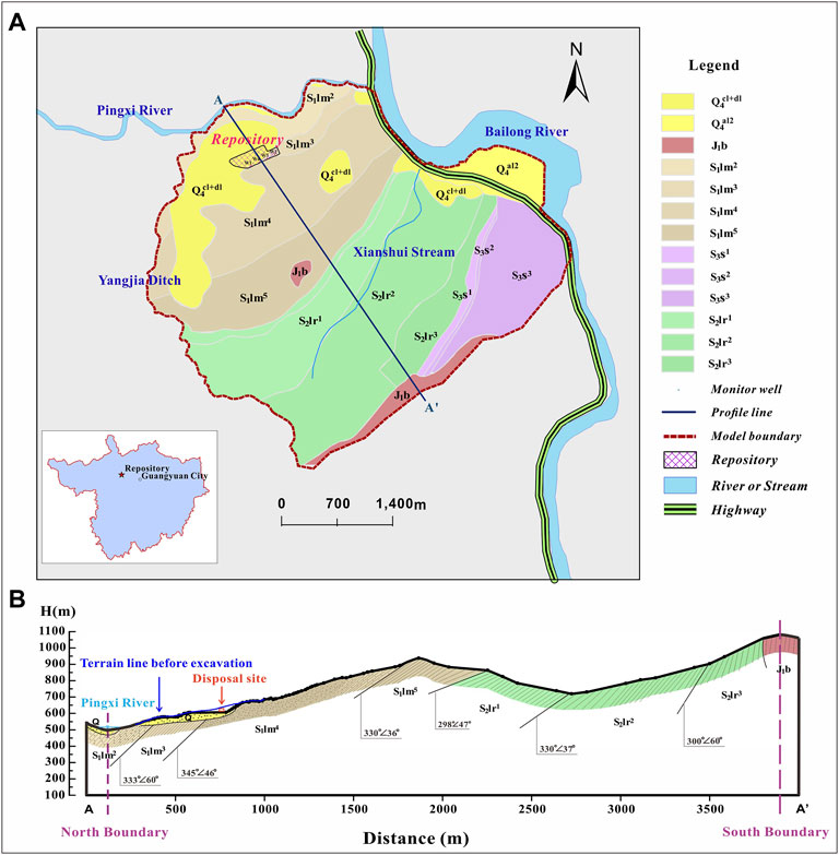
FIGURE 1. (A) Geologic map of the LILW repository study area. (B) Northwest geological section of the study area.
2.1 Geological and Hydrogeological Conditions
The disposal site was a classic example of hilly topography at an elevation about 606 m above mean sea level, underlain by shale base rock of the Silurian age. The geological drilling survey data of the study area showed that the site area’s stratigraphy was relatively simple. The argillaceous shale of the Early Jurassic and Middle-Late Silurian ages widely existed, with thin Quaternary deposits overlying in local places (Figure 1A). The previous detailed drilling data showed the strata could be divided into five sub-layers. They were Quaternary Holocene silty clay (collapse slope deposit), completely weathered argillaceous shale, highly weathered argillaceous shale, moderately weathered argillaceous shale, and slightly weathered argillaceous shale top-down (Table 1). In weathered argillic shale, fractures developed pretty well. According to the near-surface survey of fractures, the main characteristics of fractures in the site were small joints with steep dip angles.
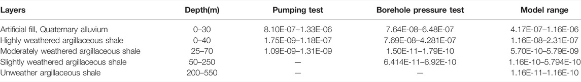
TABLE 1. Hydraulic conductivity of layers calculated from previous tests (unit: m/s).
In contrast with 35 types of fractured rock masses classified by the International Society for Rock Mechanics (Lili, 2011), fractures developed in weathered argillic shale of this study area mainly belonged to Low Ductility and Medium Interval type, followed by Medium Ductility and Medium Interval type. Lili (2011), Zhang et al. (2017) once used FractureToKarst software to analyze the existence and size of REV of the 35 types of fractured rock according to the criterion that the permeability coefficient does not change dramatically with the change of the study range. The REV of the Low Ductility and Medium Interval and Medium Ductility and Medium Interval type fractured rocks were 30.0 m × 15.0 m and 10.0 m × 5.0 m.
The site’s groundwater was mainly weathered fissure water with a depth of 5–30 m, distributed in a plane shape and controlled by landform. The primary groundwater sources were atmospheric precipitation recharge, surface trench water, and groundwater recharge from the overlying quaternary aquifer of local places. They discharged to surface streams, Bailong River or Pingxi River.
2.2 Artificial Facilities
In this research, artificial facilities like covering layers and drainage facilities were the main components considered in groundwater flow modeling. In this study, the covering layers of the disposal units consisted of four sub-layers, which were the vegetable layer (VL), the water-retaining layer (WRL), the clay layer (CL), and the local soil layer (LSL), respectively (Figure 2A).In addition, several seepage ditches had been set around the site, and inclined drainage holes had been arranged along the slope (Figure 2B). Moreover, as time goes by, the drainage hole could be blocked by sands and gravel, and the seepage ditches would be deformed and damaged due to geological processes and bio disturbance. Therefore, three states describe their aging and failure processes were defined. The first was the sound state, which means these artificial facilities work normally and drain smoothly. The second state was an altered state. In this state, some of these facilities had problems gradually, and drain occurred difficultly. The last state was called the degraded state, where all of these facilities were invalided and drained void. In this study, the 2,150 and 2,350 were supposed to be the time nodes according to the lifetime of these installations (Figure 3). After 2,150, half of the drainage installations were assumed lost efficacy. Then, by 2,350, the drainage system was ultimately out of work. These states were essential references for subsequent multi-stage modeling.
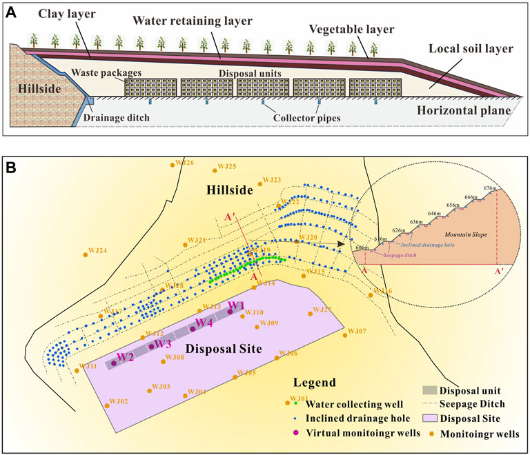
FIGURE 2. (A) The disposal units' generalized structure of the LILW repository. (B). Schematic diagram of artificial drainage facilities.
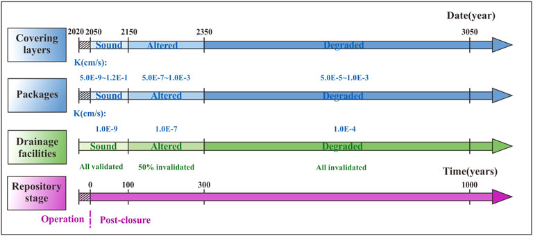
FIGURE 3. Time phase and states of main facilities components in simulations.
3 Modeling Method and Setting
In total four time-continuous groundwater flow models were established following the state’s changes to the disposal repository. The first flow model was the current flow model, which aimed to simulate the flow dynamics from operation to closure of the disposal repository. The covering layer was not formed in this period. The second one was called the sound stage flow model. Because of the addition of the covering layer, the model structure needed to be adjusted. In this period, the drainage facilities ran smoothly, and the lithology of the covering layer and disposal unit was also stable. Hence, the hydraulic parameters were at their original value in simulation. The third flow model was defined as the altered state flow model. Due to the degradation of the artificial facilities and disposal materials, the drainage structures, hydraulic parameters of the disposal unit, and covering layer were needed to make the corresponding adjustments. The last was the degraded state model, with artificial drainage facilities failing; the covering layer and disposal unit materials were wholly degraded and homogenized. The hydraulic parameters should be adjusted along with the change of the artificial facilities states in simulations. The specific and critical model settings were described as follows:
3.1 Model Scope and Boundary Conditions
The extent of the regional model was decided by the hydrological conditions of the mountain area. Pingxi river in the north of the disposal site flowed into the Bailong River from west to east. The inlet was at the northeast corner of the disposal site. Therefore, the two fixed head boundaries were determined by a north river and a river in the northeast. In addition, it was surrounded by a natural surface ditch and ridge along the west and south boundaries, which made the region an essentially isolated hydrogeologic unit (Figure 1A). A high hill in the south could be considered an impermeable boundary (Figure 1B). The west boundary was determined by a natural ditch called Yangjia Ditch as a mixed boundary (Figure 1A). The primary river Pingxi River, from west to east, was simulated as a head-dependent flow boundary. A stream named Xianshui Stream was in the middle of the study area (Figure 1A). It was treated as a drainage ditch boundary in simulations because it didn’t exist a stable water level all along. After being recharged by precipitation, the groundwater flowed from the hilly area to the foot of the hills and discharged mainly into the Pingxi River, and then flowed out through the Bailong River.
3.2 Grid Structure and Seepage Boundary
According to the lithology of the study area, the whole model was vertically divided into nine layers. Grid encryption was carried out in the disposal site area and the rivers. Cells’ size (side length) was generally 50–100 m in most study areas and was encrypted in the disposal area by less than 15 m. Moreover, the model structure changed when adding the covering layers above the disposal units. Showed in Figure 4A, after adding the covering layers, the covering layer’s cells needed to overlay the disposal unit’s cells in the model structure.
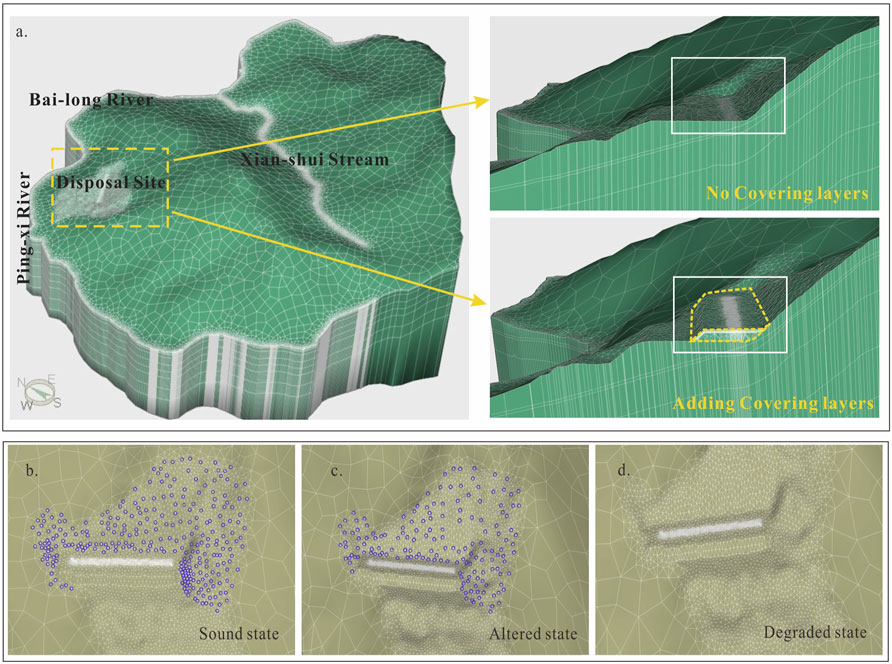
FIGURE 4. (A) Schematic graphs of space discretization before and after adding covering layers. (B–D): Simulation of drainage facilities under different states.
Seepage boundaries were used to simulate the drainage facilities, and they would change along with three different states. In the sound state, the seepage boundaries were set at all the locations of drain holes (Figure 4B). The drainage facilities were supposed to lose efficacy at an altered state, so there were half holes being chosen uniformly and randomly to keep seepage boundaries (Figure 4C). In the degraded state, the drainage facilities were assumed to be invalid. Therefore, we canceled the seepage boundaries in this period, as shown in Figure 4D.
3.3 Hydraulic Conductivities
The mathematical models for groundwater flow in fractured media mainly included the following:
The equivalent continuous media model
Discrete fracture network model
Dual media model
Coupling model
Each one had its applicable conditions. If REV (Representative Element Volume) existed in the study fracture area and was small enough compared with the scale of the study area, the equivalent continuum model can be used to describe the groundwater movement in this fractured media (Zhifang, 2007). According to this, we contrasted the range of study areas and the REV of weathered argillic shale. The REV was less than 30 m × 15 m based on Lili Zhang’s research (Lili, 2011), and the study area was about 13.1 km2, more than two orders of magnitude both in width and length. Therefore, an equivalent continuous medium was used to generalize fractured media in this study. The whole study area was generalized into the heterogeneous, three-dimensional, and transient groundwater flow system.
Therefore, the rock, soils, and artificial disposal facilities in the site area were generalized as the equivalent continuous isotropic medium in this study. Table.1 showed the value range assigned for the dirt and rock layers according to the rock hydraulic properties and previous field hydraulic testing results by the preliminary site investigation from the Beijing Research Institute of Uranium Geology (BRIUG). Also,these parameters were regarded as invariant over time.
Considering the covering layers’ designed structure and possible future degradation for artificial facilities, the covering layers were subdivided into six layers for different filling materials based on four sub-layers (Figure 2A). Three aging states (Figure 3) were assumed. Six layers, including one vegetable layer (VL), three water-retaining layers (WRL), one clay layer (CL), and one local soil layer (LSL). Three aging states included sound state, altered state, and degraded state. The material parameters in every state were uniform and steady in simulations. So, different hydraulic conductivity values were assigned to characterize its hydraulic properties and aging state at various future times according to the material’s property (Table 2).
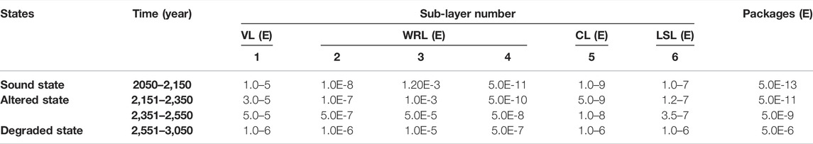
TABLE 2. Hydraulic conductivity of covering sub-layers and packages under different states (unit: m/s).
3.4 Precipitation
The primary recharge source of groundwater in the study area was atmospheric precipitation infiltration. According to the different outcropping lithology and the influence of topographic slope, the annual rainfall recharge in the study area was divided and calculated by giving different infiltration coefficients. For a long-term assessment with a thousand-year scale, more factors could affect the climate and precipitation. According to a peer meteorological particular study had been conducted by the Institute of Earth Environment, four Representative Concentration Pathways Climate Scenarios (RCPs) were designed based on multiple earth system models: RCP2.6, RCP4.5, RCP6.0, and RCP8.5, corresponding to very low, low, moderate, and high greenhouse gas (GHG) emissions conditions, respectively. In each RCPs climate scenario, there was a corresponding precipitation curve over time. The RCPs4.5 climate scenario was the most usual and comparatively conservative scenario therein. Thus, the rainfall under RCPs 4.5 climate scenario was chosen in future prediction simulations. As Figure 5 showed, the precipitation had an overall increasing trend in the future. Before 2,100, the rainfall rose sharply, and after 2,100, the amount of rain fluctuated remarkably, ranging from 910.16 to 2,201.08 mm/y. After 2,550, the precipitation value became sparse, with one per decade. Hence, the rainfall values were supposed to be the same every decade during simulations.
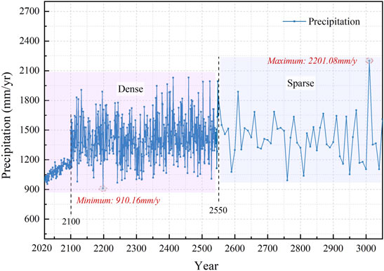
FIGURE 5. Predicted precipitation curve in Rcps4.5 (Low GHG emissions condition of Representative Concentration Pathway Climate Scenario) by Institute of Earth Environment, Chinese Academy of Sciences.
4 Results and Discussion
4.1 Model Calibration
The flow equilibrium analysis and the fitting comparison between the actual and simulated hydraulic head of boreholes were used to identify and calibrate the current mode. After numerous adjusting parameters, the current model had an equilibrium in recharge and discharge, and the water levels fitted well. The benchmark data of the steady flow groundwater level fitting was the average value of the stable water levels in the dry and wet seasons from 2016 to 2020. Nine representative monitor boreholes located near the disposal site were analyzed. The mean absolute error was 1.5 m and the square of correlation coefficient R2 = 0.99 ≈ 1, which means the simulated water levels were very close to the actual situation. Figure 6A showed the fitting diagram of measured and observed values, and each point was very close to the line, indicating that the simulation value made a pretty good agreement with the measured data.

FIGURE 6. (A) Fitting diagram of groundwater observation wells in steady flow. (B–D) Fitting diagram of groundwater observation wells WJ02, WJ17, and WJ24 in transient flow.
After the calibration of transient flow, the groundwater flow model can better simulate the dynamic change of groundwater in the study area and reproduce the response process of groundwater to rainfall. The monitoring water level data from 2016 to 2020 were used for identification and verification. Figures 6B–D showed the dynamic fitting results of water level of observation wells WJ02, WJ17, and WJ24. The variation trends of simulated and observed water levels were the same by comparing the process line of simulated and measured water levels. The fluctuations of unreal water levels were basically in accord with the changes in rainfall. In conclusion, the steady and unsteady water level fitting results reached the general fitting goals.
4.2 Groundwater Level Prediction and Analysis
4.2.1 Groundwater Level
To better understand groundwater levels of the disposal units, four virtual monitoring points in disposal units were set (locations of W1, W2, W3, and W4 can be seen in Figure 2B). As the variation curves showed, the change of hydraulic head had a linear increase in the operation stage (years 2020–2050) of the disposal units (Figure 7①, which is in accordance with the change in rainfall.
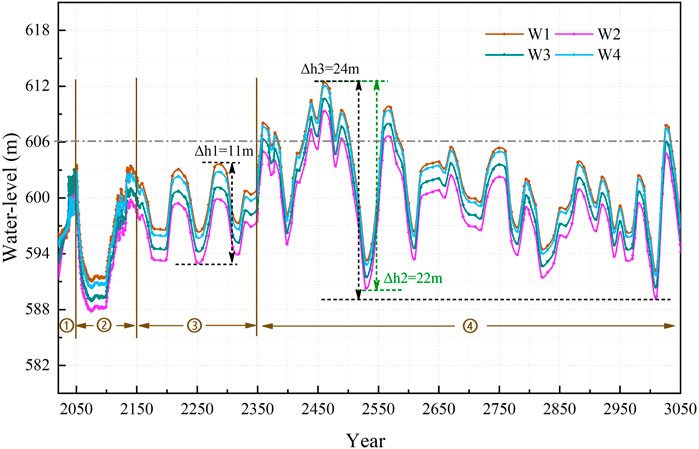
FIGURE 7. Variation curves of groundwater levels of LILW repository from 2,020 to 3,050.
In 2,050, the disposal units will be manually covered. The sound state was defined from 2050 to 2,150 while all artificial facilities were under regular operation (covering layers and waste packages were not degraded, and drainage facilities are fully operational). As a result, the groundwater levels dropped rapidly in this period (Figure 7②). It was possible because the small waterproof space formed as the instantly adding covering layers during simulation. That would bring less infiltration. However, as the rainfall increased and the surrounding continuous groundwater recharge, groundwater began to recover gradually, and by 2,150, it nearly reached the level before adding the covering layers.
After that, the artificial facilities were supposed to come into an altered stage (from 2,150 to 2,350, Figure 3). In this stage, half of the drain facilities stochastically occurred plugging or blocking after more than 100 years’ use. The covering layers and packages’ material hydraulic properties had aging problems (Figure 3). The resulting curve showed the groundwater appeared to have a similar fluctuation shape variation to the precipitation change, and the range of fluctuation was 11 m (Figure 7③,
After 2,350, all artificial facilities were assumed under the complete degradation stage, which means the drainage facilities completely failed. It can be seen that the change in water level had a more significant fluctuation than that in the altered stage by a fluctuation range of 24 m (Figure 7④,
Above all, it can be concluded that the groundwater level of the disposal unit was basically controlled by precipitation, especially the drainage facilities had a particular regulating effect on the groundwater level, which can cut down the fluctuation impact brought by rainfall’s fluctuation to some degree by lowering the maximum amplitude of groundwater level variation at the disposal site from 22 m (Figure 7,
4.2.2 Flow Field
In the region flow, shallow water generally flowed from south to north, controlled by rainfall and topography, and drained into rivers and gullies from the top places of the terrain. According to the plane, the flow field shown in Figure 8A, Pingxi River, Bailong River, Xianshui Stream, and Yangjia Ditch were discharge sites. The groundwater flow direction was north for the disposal area, flowing from the south slope to the Pingxi River. It can be seen from the northwest section flow field (Figure 8B) that there were double groundwater flow systems in the study area: the local and regional groundwater flow systems. The groundwater in the disposal area participated in a local groundwater flow system circulation, which was mainly supplied by the rainfall on the high places of the adjacent slope and flowed into the Pingxi River along the north, and the circulation depth was shallow (depth less than 300 m). In addition, the Xianshui Stream, as the main outlet, belonged to another local groundwater flow system. Groundwater flowed from both sides of higher places to it. The rainfall in the Hejia Mountain area would also flow deep underground (minimum depth of over 500 m) and drained into the Pingxi River, forming a regional groundwater flow system.
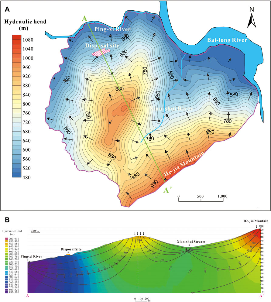
FIGURE 8. (A) Flow field diagram of the study area in 2,150. (B) Flow field profile in the northwest direction in 2,150.
4.2.3 Particle-Tracking Test
To know the time groundwater flowing from the disposal site to Pingxi River would spend, some water particles in the aquifer under the disposal units were set to figure out the possible runoff path and the travel time flowing to outlets based on the current model. The results showed the particles would flow north into the Pingxi River, and the whole process took less than 25.99 years. The fastest particle took less than 19.49 years (Figure 9). Along with these path lines, the depth of the groundwater level was getting smaller and smaller. Also, the range of the depths is mainly in the top two layers, ranging from 0 to 45 m.
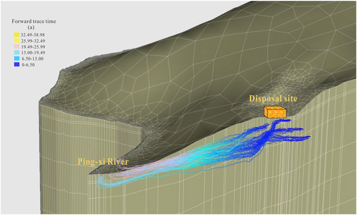
FIGURE 9. Particles’ travel lines from the aquifer beneath the repository to the Pingxi River.
4.3 Uncertainty Analysis of Groundwater Flow Model Parameters
Due to the uncertainty of the input parameters of the flow model, the sensitive parameters of groundwater level and the change ranges and characteristics of groundwater level caused by the possible variety of the sensitive parameters were further analyzed.
4.3.1 Sensitivity Analysis
The factor transformation method of a local sensitivity analysis method was used to determine sensitive parameters and partition parameters in the groundwater flow models. In models, permeability coefficient, rainfall infiltration coefficient, and water storage coefficient were the main considered parameters. As shown in Figures 10A,B, the sensitivity of the permeability coefficient was the highest, the sensitivity of the infiltration coefficient was the second, and the sensitivity of the water storage coefficient was the lowest. And the most significant sensitivity area of the three corresponding parameters was chosen as the sensitive variable for the subsequent uncertainty analysis. Taking the permeability coefficient, for example (Figure 10C), the 12th permeability coefficient partition had the most considerable sensitive value, so the permeability coefficient in the 12th partition was determined to be the sensitive variable. The same method determined the most sensitive infiltration and water storage coefficient zones.
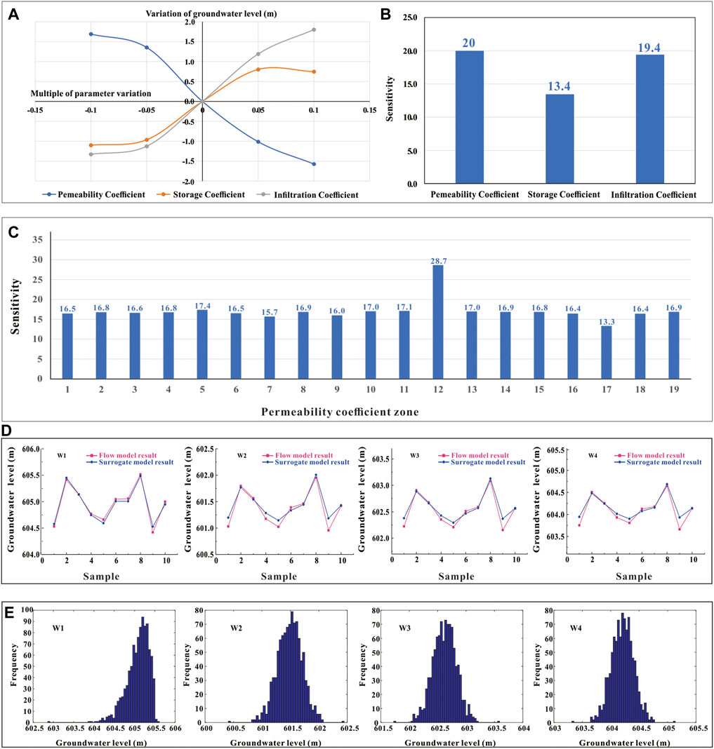
FIGURE 10. (A,B). Groundwater level variation diagram and sensitivity histogram. (C). Sensitivity histogram of all permeability coefficient zones. (D). Fitting results of groundwater levels of four virtual monitoring holes (W1, W2, W3, W4) between the 2,150 years’ surrogate model and groundwater flow model. (E). Frequency distributions of groundwater level terms by the 2150-years surrogate model.
4.3.2 Surrogate Models
Due to the time-consuming operation of the four flow models, it would take a lot of time to conduct thousands of simulations. Therefore, to save calculation time, three surrogate models were built to analyze groundwater levels condition in 2,150, 2,350, and 3,050 years, respectively. The surrogate models’ construction process included: 1) Generation of 50 samples for each surrogate model. The procedures involved using the Latin Hypercube Sampling method (Zhang and Pinder, 2003) to obtain 50 groups of model parameters and then inserting them into the groundwater numerical model to get the water level results in four virtual monitoring wells of the disposal site. 2) Using the Support Vector Regression (SVR) method (Bozorg-Haddad et al., 2020) to train the surrogate model based on the randomly chosen 40 groups of model parameters and the running result values in the 50 groups of samples. 3) Surrogate model testing. The remaining ten groups of sample parameters and running results were used to verify the accuracy of the surrogate models. Taking the 2150-year surrogate model as an example, shown in Figure 10D, the results of the groundwater level of four virtual monitoring holes fitted well with the surrogate model. The mean square error MSE was small, the maximum was not more than 0.0016, and the determinate coefficients R2 were above 0.92. These data indicated the established support vector regression model had high precision and met the requirements of calculation, which can approximately replace the function of groundwater flow models. The 2350-and 3050-years surrogate models fitted well with the flow models as well, and the accuracy calculation results of the three surrogate models were shown in Table 3.
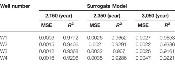
TABLE 3. Water level errors between surrogate models and groundwater flow models.
4.3.3 Uncertainty Analysis Results
Using the Latin Hypercube Sampling method to obtain 1,000 samples according to the probability distribution characteristics of random variables, three surrogate models were used to calculate the groundwater level results. After that, the SPSS software was used to conduct the K-S test for the prediction results. The statistical indexes result can see in Table 4. The frequency distribution characteristics of groundwater levels in 2,150, 2,350, and 3,050 years showed in Figure 10E. The frequency distributions of groundwater levels were Skewed and Normal distribution. And the confidence interval and the range of groundwater level variation can be calculated according to these frequency distributions.
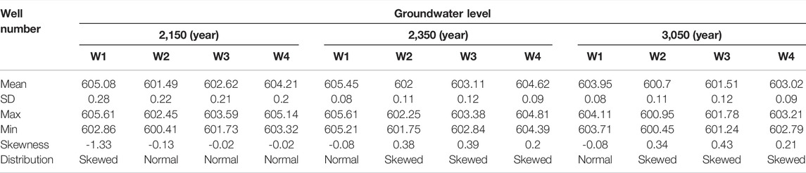
TABLE 4. Frequency distributions characteristics of groundwater level terms predicted by three time period surrogate models.
As Table.5 showed, in 2,150, the groundwater level of four virtual observation wells had a 95% probability of being between 601.13 and 605.54 m. In 2,350, the water levels of four virtual observation well had a 95% probability of being between 601.82 and 605.58 m. In 3,050, the water level of virtual observation wells was between 600.52 and 604.08 m, which was all lower than the elevation of the disposal platform.
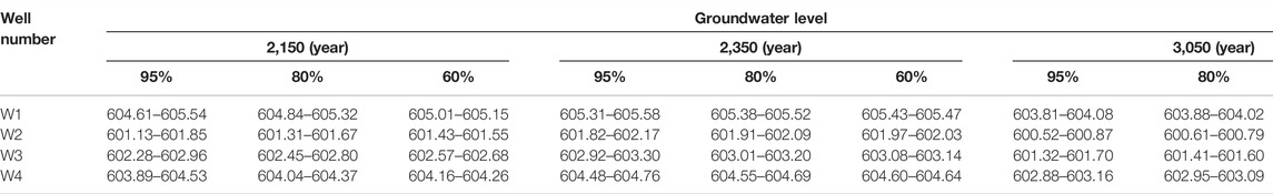
TABLE 5. Confidence interval of groundwater levels in 2,150, 2,350, and 3,050.
5 Conclusion
In this study, a set of groundwater flow models at the regional scale was constructed to analyze and predict the possible change in groundwater within a millennial scale. The models considered the artificial facilities’ function and potential alterations, including the adequate, partial failure, and complete failure drainage facilities, the addition of the covering layer, and the degradation of disposal unit materials over time. The results showed groundwater level of the disposal unit was basically controlled by precipitation, especially the drainage facilities had a particular regulating effect on the groundwater level, which can cut down the fluctuation impact brought by rainfall fluctuation to the degree of lowering the maximum amplitude of groundwater level variation at the disposal site from 22 to 11 m under roughly the same rainfall fluctuation. Therefore, the drainage facilities can protect the disposal units from soaking groundwater. Keeping them effective can help store radioactive waste. From the perspective of store safety in radioactive waste and groundwater, we made sensitivity and uncertainty analysis to predict the groundwater level range and probability in 2,150, 2,350, and 3,050. Also, we assessed the groundwater circulation process and expected the groundwater migration time from the disposal site to the discharge area by the current model. The main conclusions from this study include:
Long-term flow models showed that groundwater levels would not be beyond the bottom of the repository before 2,350. But after 2,350, when the rainfall was more significant than 1950 mm/y for 10 years, all the drainages lost efficacy, and the groundwater level would be higher than the bottom surface of the disposal units. The uncertainty analysis results showed that in 2,150, the groundwater levels of four virtual observation wells had a 95% probability of being between 601.13 and 605.54 m. In 2,350, the groundwater levels of virtual observation wells had a 95% probability of being between 601.82 and 605.58 m. In 3,050, the groundwater levels of virtual observation wells were between 600.52 and 604.08 m, all lower than the elevation of the disposal platform with a height of 606 m. The groundwater in the disposal area participated in a local groundwater flow system circulation, which was mainly supplied by the rainfall on the high places of the adjacent slope and flowed into the Pingxi River along the north, and the circulation depth was shallow (depth less than 300 m). Particle-tracking numerical tests showed the particles would flow north into the Pingxi River, and the whole process took less than 25.99 years. The fastest particle took less than 19.49 years.
This work was a critical regional groundwater flow modeling case for the long-term safety assessment of a particular LILW near-surface disposal repository. These results can provide a basis for further analysis of radioactive waste migration range and time, and also provide references for regional flow modeling processes in near-surface disposal engineering. Besides, there were some deficiencies in this work. In the time nodes given, they were subjectively defined according to the service life of artificial facilities, but the time is uncertain. Therefore, how to deal with the uncertainties is a meaningful research topic for radioactive disposal safety in the future.
Data Availability Statement
The original contributions presented in the study are included in the article/Supplementary Material; further inquiries can be directed to the corresponding author.
Author Contributions
HZ: drafting the manuscript. QZ: revising and editing the manuscript. YuC: data collection and provision of the study area. JS: development or design of the methodology. YaC: site survey and data analysis. WW: building flow models. SH: uncertainty analysis.
Funding
This work was supported by the project of Systematic Analysis of the whole safety process of Low and Medium Radioactive Solid Waste Disposal Site in Fei-feng Mountain.
Conflict of Interest
Author YC was employed by CNNC Everclean Environmental Engineering Co., Ltd.
The remaining authors declare that the research was conducted in the absence of any commercial or financial relationships that could be construed as a potential conflict of interest.
Publisher’s Note
All claims expressed in this article are solely those of the authors and do not necessarily represent those of their affiliated organizations, or those of the publisher, the editors, and the reviewers. Any product that may be evaluated in this article, or claim that may be made by its manufacturer, is not guaranteed or endorsed by the publisher.
Acknowledgments
The authors are grateful to the peer climate studies by the Institute of Earth Environment, Chinese Academy of Sciences, and fracture and hydraulic test results data from Nuclear Industry Southwest Geotechnical Investigation and Design Institute Co., Ltd.
References
Ashraf, A., and Ahmad, Z. (2008). Regional Groundwater Flow Modelling of Upper Chaj Doab of Indus Basin, Pakistan Using Finite Element Model (Feflow) and Geoinformatics. Geophys. J. R. Astronomical Soc. 173 (1), 17–24. doi:10.1111/j.1365-246X.2007.03708.x
Birkholzer, J. T., Tsang, C.-F., Bond, A. E., Hudson, J. A., Jing, L., and Stephansson, O. (2019). 25 Years of DECOVALEX - Scientific Advances and Lessons Learned from an International Research Collaboration in Coupled Subsurface Processes. Int. J. Rock Mech. Min. Sci. 122 (122), 103995. doi:10.1016/j.ijrmms.2019.03.015
Bozorg-Haddad, O., Delpasand, M., and Loáiciga, H. A. (2020). Self-optimizer Data-Mining Method for Aquifer Level Prediction. Water supply 20 (2), 724–736. doi:10.2166/ws.2019.204
Bracke, G., and Fischer-Appelt, K. (2015). Methodological Approach to a Safety Analysis of Radioactive Waste Disposal in Rock Salt: An Example. Prog. Nucl. Energy 84, 79–88. doi:10.1016/j.pnucene.2015.01.012
Bracke, G., Kudla, W., and Rosenzweig, T. (2019). Status of Deep Borehole Disposal of High-Level Radioactive Waste in Germany. Energies 12, 2580. doi:10.3390/en12132580
Bugai, D., Skalskyy, A., Dzhepo, S., Kubko, Y., Kashparov, V., Van Meir, N., et al. (2012). Radionuclide Migration at Experimental Polygon at Red Forest Waste Site in Chernobyl Zone. Part 2: Hydrogeological Characterization and Groundwater Transport Modeling. Appl. Geochem. 27 (27), 1359–1374. doi:10.1016/j.apgeochem.2011.09.028
Chapman, N. (2019). Who Might Be Interested in a Deep Borehole Disposal Facility for Their Radioactive Waste? Energies 12, 1542. doi:10.3390/en12081542
Cornelissen, T., Diekkrüger, B., and Bogena, H. (2016). Using High-Resolution Data to Test Parameter Sensitivity of the Distributed Hydrological Model Hydrogeosphere. Water 8 (5), 202. doi:10.3390/w8050202
Darda, S. A., Gabbar, H. A., Damideh, V., Aboughaly, M., and Hassen, I. (2021). A Comprehensive Review on Radioactive Waste Cycle from Generation to Disposal. J. Radioanal. Nucl. Chem. 329 (1), 15–31. doi:10.1007/s10967-021-07764-2
De Caro, M., Crosta, G. B., and Previati, A. (2020). Modelling the Interference of Underground Structures with Groundwater Flow and Remedial Solutions in Milan. Eng. Geol. 272, 105652. doi:10.1016/j.enggeo.2020.105652
Deng, D., Zhang, L., Dong, M., Samuel, R. E., Ofori‐Boadu, A., and Lamssali, M. (2020). Radioactive Waste: A Review. Water Environ. Res. 92, 1818–1825. doi:10.1002/wer.1442
Fu, J., and Gómez-Hernández, J. (2009). Uncertainty Assessment and Data Worth in Groundwater Flow and Mass Transport Modeling Using a Blocking Markov Chain Monte Carlo Method. J. hydrology 364 (3-4), 328–341. doi:10.1016/j.jhydrol.2008.11.014
Geetha Manjari, K., and Sivakumar Babu, G. L. (2017). Probabilistic Analysis of Groundwater and Radionuclide Transport Model from Near Surface Disposal Facilities. Georisk Assess. Manag. Risk Eng. Syst. Geohazards 12, 60–73. doi:10.1080/17499518.2017.1329538
IAEA (1994). Siting of Near Surface Disposal Facilities. Vienna: International Atomic Energy Agency. IAEA Safety Series No. 111-G-3.1.
Jafari, F., Javadi, S., Golmohammadi, G., Mohammadi, K., Khodadadi, A., and Mohammadzadeh, M. (2016). Groundwater Risk Mapping Prediction Using Mathematical Modeling and the Monte Carlo Technique. Environ. Earth Sci. 75 (6), 491. doi:10.1007/s12665-016-5335-9
Jeong, J., Kown, M., and Park, E. (2018). Safety Assessment of Near Surface Disposal Facility for Low-And Intermediate-Level Radioactive Waste (LILW) through Multiphase-Fluid Simulations Based on Various Scenarios. Econ. Environ. Geol. 2 (51), 131–147. doi:10.9719/EEG.2018.51.2.131
Klein, E., Hardie, S. M. L., Kickmaier, W., and McKinley, I. G. (2021). Testing Repository Safety Assessment Models for Deep Geological Disposal Using Legacy Contaminated Sites. Sci. Total Environ. 776, 145949. doi:10.1016/j.scitotenv.2021.145949
Kozak, M. W. (2017). “Safety Assessment for Near-Surface Disposal of Low and Intermediate Level Wastes,” in Geological Repository Systems for Safe Disposal of Spent Nuclear Fuels and Radioactive Waste. Second Edition, 475–498. doi:10.1016/b978-0-08-100642-9.00016-5
Lee, S., and Kim, J. (2017). Post-closure Safety Assessment of Near Surface Disposal Facilities for Disused Sealed Radioactive Sources. Nucl. Eng. Des. 313, 425–436. doi:10.1016/j.nucengdes.2017.01.001
Li, X., Li, D., Xu, Y., and Feng, X. (2020). A DFN Based 3D Numerical Approach for Modeling Coupled Groundwater Flow and Solute Transport in Fractured Rock Mass. Int. J. Heat Mass Transf. 149, 119179. doi:10.1016/j.ijheatmasstransfer.2019.119179
Lili, Z. (2011). Determining the Representative Elementary Volumes of Fracture Rock Mass Based on Permeability Analysis. Beijing: China university of geoscience, 20–111. (in Chinese).
Michie, U. M. (1998). Deep Geological Disposal of Radioactive Waste A Historical Review of the UK Experience. Interdiscip. Sci. Rev. 23 (2), 242–257. doi:10.1179/isr.1998.23.3.242
Parameswaran, T. G., Anusree, N., Sughosh, P., Sivakumarbabu, G. L., and Deepagoda, T. K. K. C. (2021). Suitability of Mechanically Biologically Treated Waste for Landfill Covers. Lect. Notes Civ. Eng. 144, 511–519. doi:10.1007/978-981-16-0077-7_44
Santos, J. E., Xu, D., Jo, H., Landry, C. J., Prodanović, M., and Pyrcz, M. J. (2020). Poreflow-net: A 3D Convolutional Neural Network to Predict Fluid Flow through Porous Media. Adv. Water Resour. 138, 103539. doi:10.1016/j.advwatres.2020.103539
SKB (2013). Flow Modelling on the Repository Scale for the Safety Assessment. SDM-PSU Forsmark. Stockholm: Svensk Kärnbränslehantering AB. SKB TR-13-08.
SKB (2014). Flow and Transport Modelling on the Vault Scale. SDM-PSU Forsmark. Stockholm: Svensk Kärnbränslehantering AB. SKB TR-14-14.
Sreekanth, J., Crosbie, R., Pickett, T., Cui, T., Peeters, L., Slatter, E., et al. (2020). Regional-scale Modelling and Predictive Uncertainty Analysis of Cumulative Groundwater Impacts from Coal Seam Gas and Coal Mining Developments. Hydrogeol. J. 28 (1), 193–218. doi:10.1007/s10040-019-02087-9
Watson, C., Wilson, J., Savage, D., and Norris, S. (2018). Coupled Reactive Transport Modelling of the International Long-Term Cement Studies Project Experiment and Implications for Radioactive Waste Disposal. Appl. Geochem. 97, 134–146. doi:10.1016/j.apgeochem.2018.08.014
Welch, E. M., Dulai, H., El-Kadi, A., and Shuler, C. K. (2019). Submarine Groundwater Discharge and Stream Baseflow Sustain Pesticide and Nutrient Fluxes in Faga'alu Bay, american samoa. Front. Environ. Sci. 7, 162. doi:10.3389/fenvs.2019.00162
Yi, S., Ma, H., Zheng, C., Zhu, X., Wang, H. a., Li, X., et al. (2012). Assessment of Site Conditions for Disposal of Low- and Intermediate-Level Radioactive Wastes: A Case Study in Southern China. Sci. Total Environ. 414, 624–631. doi:10.1016/j.scitotenv.2011.10.060
Yim, M.-S., and Simonson, S. A. (2000). Performance Assessment Models for Low Level Radioactive Waste Disposal Facilities: a Review. Prog. Nucl. Energy 36 (1), 1–38. doi:10.1016/S0149-1970(99)00015-3
Zhang, L., Xia, L., and Yu, Q. (2017). Determining the REV for Fracture Rock Mass Based on Seepage Theory. Geofluids 2017, 1–8. doi:10.1155/2017/4129240
Zhang, Y., and Pinder, G. (2003). Latin Hypercube Lattice Sample Selection Strategy for Correlated Random Hydraulic Conductivity Fields. Water Resour. Res. 39 (8), SBH 11. doi:10.1029/2002WR001822
Keywords: long-term safety assessment, sensitivity analysis, and uncertainty analysis, drainage facilities, FEFLOW software, groundwater level prediction
Citation: Zhang H, Zhang Q, Chen Y, Shao J, Cui Y, Wan W and Han S (2022) Groundwater Flow Modeling of a Near-Surface Disposal Repository for Low- and Intermediate-Level Radioactive Waste in Southwest China. Front. Environ. Sci. 10:917416. doi: 10.3389/fenvs.2022.917416
Received: 11 April 2022; Accepted: 28 April 2022;
Published: 13 June 2022.
Edited by:
Lichun Wang, Tianjin University, ChinaCopyright © 2022 Zhang, Zhang, Chen, Shao, Cui, Wan and Han. This is an open-access article distributed under the terms of the Creative Commons Attribution License (CC BY). The use, distribution or reproduction in other forums is permitted, provided the original author(s) and the copyright owner(s) are credited and that the original publication in this journal is cited, in accordance with accepted academic practice. No use, distribution or reproduction is permitted which does not comply with these terms.
*Correspondence: Qiulan Zhang, cWx6aGFuZzkxOUBjdWdiLmVkdS5jbg==