Modeling shallow soil moisture dynamics in mountainous landslide active regions

Under the worsening climate change, the mountainous landslide active regions are more likely to suffer severe disasters threatening residents. To predict the occurrence of landslides, shallow soil moisture lying in the interface of the hydrological processes has been found as one of the critical factors. However, shallow soil moisture data are often scarce in the landslide active regions. To overcome the severe measurement deficiencies and provide predictions of soil moisture dynamics, we construct a physically-based shallow soil moisture model based on the assumptions of ideal flow, homogeneous and isotropic soil textures, and 1-dimensional water movement dominant by gravity forces. In the model, the meteorological conditions and the physical soil properties are taken into consideration. With limited field measurements, the model can provide reasonably accurate soil moisture predictions. In recognition of the seasonal weather characteristics, we perform a series of sensitivity analyses to examine the response of shallow soil moisture and relate the hydrological processes to air temperature, precipitation intensity, duration, and combinations thereof. Complex interactions of hydrological processes are found with variations in precipitation and air temperature, depending on the interlinked boundary conditions of the soil and water. It demonstrates a strong need for a decent forecast of the complex shallow soil moisture dynamics and the associated hydrologic processes in mountain regions to cope with climate change for landslide preparation and agricultural adaptation in the future.

1 Introduction

The soil water accounts for merely 0.1% of the total water on the Earth (Strobbia and Cassiani, 2007; Ma et al., 2021). Lying in the pathway of the surface- and subsurface-hydrological processes, the soil water plays a decisive role in the transformation of water and energy falling on the Earth’s surface to regulate the level of surface runoff and groundwater recharge (Ma et al., 2021). The dynamics of the shallow soil moisture reflect the changes in the rainfall intensity, infiltration and evapotranspiration potential, and antecedent soil moisture status (Nyamgerel et al., 2022). As 50% of the plant roots are distributed within the 200 mm beneath the ground (Fan et al., 2016), shallow soil moisture is also critical for plant growth and agricultural production (Rossato et al., 2017). Moreover, the prompt response of shallow soil moisture in the unsaturated zone to climatic variations and land surface conditions (Jabbar and Grote, 2020) is a key factor to detect slope instability useful for developing early warning signals for landslide-prone regions (Lu and Godt, 2008). Under serious concerns about climate change, multi-dimensional projections of the tendency and frequency of extremes in temperature and precipitations (IPCC, 2014; Deshmukh and Singh, 2016) all demonstrate higher risks of storm-induced soil erosions or landslides (Brocca et al., 2007; Strobbia and Cassiani, 2007; Zhou et al., 2021) and drought-related issues. The increasing risks bring great challenges to landslide hazard mitigation, water scarcity preparation, and agriculture adaptations (Fan et al., 2022; Tan et al., 2022), particularly in mountain regions that are highly vulnerable to climate change.

To strengthen the understanding of shallow soil moisture for landslide mitigation, agricultural practices, or water resources management, various models have been conducted to assess the governing mechanisms or the associated interactions and interconnections of the external driving forces in the hydrological system (Soares and Almeida, 2001; Panigrahi and Panda, 2003; Brocca et al., 2017; Wang et al., 2019; Qiao et al., 2021; Tudose et al., 2021). Distinguished by the spatial scales, some focused on using the point-based characteristics of the environmental conditions, such as the soil hydraulic properties to model the soil water movement, while others considered the spatial variability of water resources to obtain the soil water distribution (Tenreiro et al., 2020). These approaches can be generally classified into data-driven and physically-based models (Devia et al., 2015). The data-driven models involve a derivation of empirical equations fitted from the historical information or the existing data to estimate the important hydrological processes. For example, the pedo-transfer functions (PTFs) applied the regression analysis and data mining approaches using data on the percentage of sand, silt, clay, bulk density, and porosity from soil surveys, to derive PTFs for simulating soil moisture contents.

In contrast, the physically-based models consider sources and mechanisms of water between surface and subsurface based on the governing physical laws and principles of the associated processes to represent the mathematical idealized functions in a real phenomenon (Ogden et al., 2015; Li and DeLiberty, 2021). Most of these models emphasize identifying the driving forces of the water movement from the surface to the vadose zone (Arnold et al., 2012; Li and DeLiberty, 2021). Widely used physically-based soil moisture models include UNSAT-H, HYDRUS-1D, and SWAT (Soil Water Assessment Tool) (Fayer, 2000; Arnold et al., 2012; Šimunek et al., 2012). Based on water balance equations, these models are capable of simulating dynamic soil moisture contents in catchments at sub-daily to multiple time scales. For example, UNSAT-H and Hydrus-1D applied the advection-dispersion equations and Richards equation to numerically simulate heat transfer processes and variably-saturated water flow (Fayer, 2000; Šimunek et al., 2012; Rassam et al., 2018). They require a considerable number of model inputs, either from core drilling, laboratory tests, or detailed site investigation (e.g., leaf area index (LAI), root depth, the wet perimeter of the drain, etc.) (Li et al., 2015; Kanzari et al., 2018; Tonkul et al., 2019). The model complexity/uncertainty is therefore increased and creates a higher level for users to start (Schwartz et al., 1990; Albright et al., 2002). The SWAT model is a continuous, semi-distributed, and processed-based river basin model for estimating changes in water quantity and quality in a catchment. SWAT is useful to evaluate the impacts of land use, land management practices, and climate change (Arnold et al., 2012; Glavan and Pintar, 2012). Nonetheless, the finest time scale of SWAT runs at the daily time scale. It cannot catch a rapid process shorter than one day. The model is designed for basin-scale simulations, which require detailed parameterization in each sub-basin unit.

Most of the existing models require adequate observation or monitoring data of the meteorological conditions, land use, and soil moisture to better predict the water movement dynamics (Pitman, 2003; Clark et al., 2015). The precipitation, air temperature, and streamflow are monitored by governmentally operated weather stations and gauges in many places and are readily available. The data requirement of land-use changes can be estimated by satellite imagery. Nonetheless, the in-situ soil moisture data are generally less available (Soares and Almeida, 2001; Panigrahi and Panda, 2003; Wang et al., 2019), especially for mountainous landslide-active areas. To accommodate the need for shallow soil moisture information in mountain regions for agricultural practices and the protection of tribe people from landslide hazards, this study aims to develop a dynamic soil moisture model that captures rapid water movement in the shallow soil layer incorporating influences from weather and the physical properties of land and soils. In this article, we describe the construction of a physically- and process-based shallow soil moisture model for advancing rapidly dynamic interactions between soil-vegetation and rainfall-water cycling feedbacks and replenish the in-situ soil moisture data in a landslide active region and a traditional tribe settlement area in the Yufeng Village, Taiwan. We implement the model with specific parameterization and evaluate the model performance. Based on the factor sensitivity analysis results, we provide general perspectives on the responses of critical hydrological processes to seasonal weather characteristics reflecting realistic variations in air temperature, precipitation duration, and intensity. Lastly, we compare our model to the existing approaches, discuss possible sources of uncertainty, and provide potential applications of the model.

2 Model description

We develop a shallow soil moisture model for mountainous landslide active regions to capture rapid water movement in the shallow unsaturated zone. The information on shallow soil moisture content is critical for plant growth and useful for identifying slope instability or slope failure. Before constructing the shallow soil moisture model, we assume that (1) soil water is ideal flow, and (2) soils with the same textures are homogeneous and isotropic. Because the landslide active region in Yufeng contains high gravel contents, we further assume that the downward water movement in the soil is dominated by gravity forces as 1-dimensional without consideration of lateral flow and capillary water to simplify the associated hydrological processes of the water cycle beneath the ground.

2.1 Model procedure

2.1.1 Step 1: Estimation of the main model components

The shallow soil moisture model is developed based on the mass balance to estimate the main model components of the hydrological processes, including precipitation (P, mm), Hortonian overland flow (q_H, mm), infiltration (I, mm), soil moisture content (θ, mm), evapotranspiration (ET, mm), percolation (q_p, mm), and saturation flow (q_s, mm) (Figure 1). The precipitation is considered the major water source in the model. The hourly observed precipitation data are used as the values of P to model the infiltration (I) and the Hortonian overland flow (q_H) as:

$\mathit{P}=\mathit{I}\mathrm{+}{\mathit{q}}_{\mathit{H}}.(1)$

FIGURE 1

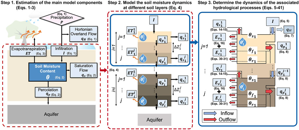
FIGURE 1. A schematic diagram showing the modeling procedures to estimate the shallow soil moisture content (θ) based on the mass balance, starting from the water sources of precipitation (P), to the various hydrological processes of the Hortonian overland flow (q_H), infiltration (I), evapotranspiration (ET), saturation flow (q_s), and percolation (q_p).

The soil moisture content (θ) can be calculated by:

$\mathit{\theta }=\mathit{I}-{\mathit{q}}_{\mathit{p}}-{\mathit{q}}_{\mathit{s}}-\mathit{E}\mathit{T}.(2)$

The evapotranspiration (ET) can be modeled as the sum of the soil evaporation (E_v, mm) and the plant transpiration (E_c, mm):

$\mathit{E}\mathit{T}={\mathit{E}}_{\mathit{v}}+{\mathit{E}}_{\mathit{c}}.(3)$

2.1.2 Step 2: Model the soil moisture dynamics at different soil layers

To model the soil moisture dynamics, we consider the soil moisture content as a dynamic equilibrium between participated inflow and outflow of water at different soil layers (Soares and Almeida, 2001; Panigrahi and Panda, 2003). As such, the soil moisture dynamics can be depicted by the infiltrated water minus any kind of outflows at any position of the soil layer at a specific time (Lane and Nearing, 1989):

${\mathit{\theta }}_{\mathit{i}}^{\mathit{j}}={\mathit{\theta }}_{0_{\mathit{i}}}^{\mathit{j}}+\mathbf{\Delta }{\mathit{\theta }}_{\mathit{i}}^{\mathit{j}}={\mathit{\theta }}_{0_{\mathit{i}}}^{\mathit{j}}+{\displaystyle \sum \left(\mathit{I}-{\mathit{q}}_{{\mathit{p}}_{\mathit{i}}}^{\mathit{j}}-{\mathit{q}}_{{\mathit{s}}_{\mathit{i}}}^{\mathit{j}}-\mathit{E}{\mathit{T}}_{\mathit{i}}^{\mathit{j}}\right),}(4)$

where i is the number of soil layers with different textures, j is the number of sublayers, ${\theta }_i^j$ represents the soil moisture content at time t (mm), ${\mathit{\theta }}_{0_{\mathit{i}}}^{\mathit{j}}$ is the initial soil moisture content (mm), $\mathrm{\Delta }{\theta }_i^j$ is the change of the soil moisture content (mm), I is the infiltration (mm), ${\mathit{q}}_{{\mathrm{p}}_{\mathit{i}}}^{\mathit{j}}$ is the percolation into the deeper soil layer (mm), $E{T}_i^j$ is the evapotranspiration on the soil surface (mm), and ${\mathit{q}}_{{\mathrm{s}}_{\mathit{i}}}^{\mathit{j}}$ is the saturation flow (mm). When i = 1 and j = 1, ${\mathit{q}}_{{\mathrm{s}}_{\mathit{1}}}^{\mathit{1}}$ is called the saturation overland flow.

2.1.3 Step 3: Determine the dynamics of the associated hydrological processes based on the soil properties and the environmental settings

In step 3, we will estimate the dynamic value of I, ${\mathit{q}}_{{\mathrm{p}}_{\mathit{i}}}^{\mathit{j}}$, ${\mathit{q}}_{{\mathrm{s}}_{\mathit{i}}}^{\mathit{j}}$, and $E{T}_i^j$ in each soil layer to determine the corresponding soil moisture dynamics (Eq. 4). Below we describe the derivation of the dynamics of each hydrological component.

2.1.3.1 Infiltration (I) and Hortonian overland flow (q_H)

Darcy’s law (Darcy, 1856) and the Horton model (Horton, 1940) are often used to describe the infiltration process, which can be determined by the magnitude of precipitation (P) and the infiltration capacity of the soil (I_c, mm). I_c can be expressed by a combination of the saturated hydraulic conductivity at the surface soil layer ($K_{\mathit{s}1}$, mm h⁻¹) and the hydraulic gradient ($\frac{\mathit{d}\mathit{h}}{\mathit{d}\mathit{Z}}+1$) between the surface and the wetting front:

$\begin{array}{l}{\mathit{I}}_{\mathit{c}}={\mathit{K}}_{{\mathit{s}}_1}\cdot \left(\frac{\mathit{d}\mathit{h}}{\mathit{d}\mathit{Z}}+1\right)\cdot \mathbf{\Delta }\mathit{t},\\ \text{when }{\mathit{I}}_{\mathit{c}}<\mathit{P} ➜ \mathit{I}={\mathit{I}}_{\mathit{c}},\\ \text{when}\mathit{ }{\mathit{I}}_{\mathit{c}}\ge \mathit{P} ➜\mathit{I}=\mathit{P},\end{array}(5)$

where h is the pressure head (mm), Z is the depth (mm), and $\mathrm{\Delta }\mathit{t}$ is the time interval.

The saturated hydraulic conductivity ($K_{si}$) describes the soil water behavior within the soil-gravels mixture in the soil layer i, which can be determined by the percentage of gravel contents in the soil layer i ($b_i$, %), the saturated hydraulic conductivity of gravel ($K_g$, mm h⁻¹), and the saturated hydraulic conductivity of the soil texture classes in the soil layer i ($K_{0i}$, mm h⁻¹) (Peck and Watson, 1979):

${\mathit{K}}_{{\mathit{s}}_{\mathit{i}}}=\frac{\frac{{\mathit{K}}_{\mathit{g}}}{{\mathit{K}}_{0_{\mathit{i}}}}\left(1+2{\mathit{b}}_{\mathit{i}}\right)+2\left(1-{\mathit{b}}_{\mathit{i}}\right)}{\left(1-{\mathit{b}}_{\mathit{i}}\right)\frac{{\mathit{K}}_{\mathit{g}}}{{\mathit{K}}_{0_{\mathit{i}}}}+\left(2+{\mathit{b}}_{\mathit{i}}\right)}{\mathit{K}}_{0_{\mathit{i}}}.(6)$

The value of $K_{0i}$ is determined by soil textures and can be estimated by PTFs (Peck and Watson, 1979).

When P exceeds the infiltration capacity, q_H occurs horizontally across land and can be caculated by substituing Eq. 5 for Eq. 1 as:

${\mathit{q}}_{\mathit{H}}=\mathit{P}-\mathit{I}=\mathit{P}-{\mathit{K}}_{{\mathit{s}}_1}\cdot \left(\frac{\mathit{d}\mathit{h}}{\mathit{d}\mathit{Z}}+1\right)\cdot \mathbf{\Delta }\mathit{t}.(7)$

2.1.3.2 Percolation (q_p) and saturation flow (q_s)

When water infiltrates the soil, two types of percolation ($q_p$) can occur, including the saturated and unsaturated water movements, which define the soil permeability (Haverkamp et al., 2016). When combining Darcy’s law with Richards equation, the saturated flow in the porous media of soils can be seen as a steady flow. Consequently, water movements at different depths can be captured by the hydraulic conductivity ($K$, mm h⁻¹) and the gradient of the pressure head in a short time period (Richards, 1931; Arampatzis et al., 2011). As such, in a very thin sublayer, the percolation flux ${\mathit{q}}_{{\mathrm{p}}_{\mathit{i}}}^{\mathit{j}}$ can be depicted as:

${\mathit{q}}_{{\mathit{p}}_{\mathit{i}}}^{\mathit{j}}={\mathit{K}}_{\mathit{i}}^{\mathit{j}}\left[\left(\frac{{\mathit{h}}_{\mathit{i}}^{\mathit{j}-1}-{\mathit{h}}_{\mathit{i}}^{\mathit{j}}}{{\mathit{Z}}_{\mathit{i}}^{\mathit{j}-1}-{\mathit{Z}}_{\mathit{i}}^{\mathit{j}}}\right)+1\right]\cdot \mathbf{\Delta }\mathit{t},\left({\mathit{\theta }}_{{\mathit{s}}_{\mathit{i}}}-{\mathit{\theta }}_{{\mathit{f}}_{\mathit{i}}}\right)\ge {\mathit{q}}_{{\mathit{p}}_{\mathit{i}}}^{\mathit{j}}\ge \left({\mathit{\theta }}_{\mathit{i}}^{\mathit{j}}-{\mathit{\theta }}_{{\mathit{f}}_{\mathit{i}}}\right),(8)$

where i is the number of soil layers with different textures, j is the number of sublayers, $K_i^j$ represents the hydraulic conductivity for saturated and unsaturated conditions to capture the movement of water in different soil textures, $\left(h_i^{j-1}-h_i^j\right)$ represents the pressure head loss, and $\left(Z_i^{j-1}-Z_i^j\right)$ is the depth difference between the sublayers of j and j-1. The percolation (q_p) deals with the gravitational water movements. When q_p occurs, ${\theta }_i^j$ will be greater than or at least equal to the field water content (${\theta }_{fi}$, mm), and will eventually reach the saturated water content (${\theta }_{si}$, mm) as the upmost constraint for ${\mathit{q}}_{{\mathrm{p}}_{\mathit{i}}}^{\mathit{j}}$.

The hydraulic conductivity ($K_i^j$) is used to represent the associated hydraulic conductivity in specific soil textures under the saturated or unsaturated conditions. The magnitude of $K_i^j$ has been found to fluctuate with the soil moisture content ${\theta }_i^j$ (Mualem, 1976), and can be calculated by the following equations (Mualem, 1976; Vereecken, 1995):

${\mathit{K}}_{\mathit{i}}^{\mathit{j}}=\left({\mathit{S}}_{{\mathit{e}}_{\mathit{i}}}^{\mathit{j}}\right){\hspace{0.17em}}^{\frac{1}{2}}{\left[\frac{{{\displaystyle \int }}_0^{{\mathit{\theta }}_{\mathit{i}}^{\mathit{j}}}\frac{1}{{\mathit{h}}_{\mathit{i}}^{\mathit{j}}}\mathit{d}{\mathit{\theta }}_{\mathit{i}}^{\mathit{j}}}{{{\displaystyle \int }}_0^{{\mathit{\theta }}_{{\mathit{s}}_{\mathit{i}}}}\frac{1}{{\mathit{h}}_{\mathit{i}}^{\mathit{j}}}\mathit{d}{\mathit{\theta }}_{\mathit{i}}^{\mathit{j}}}\right]}^2\cdot {\mathit{K}}_{{\mathit{s}}_{\mathit{i}}},(9)$

where $K_{si}$ is the hydraulic conductivity under the saturated condition, and ${\mathit{S}}_{{\mathit{e}}_{\mathit{i}}}^{\mathit{j}}$ is the fraction of water in the pore space (unitless). ${\mathit{S}}_{{\mathit{e}}_{\mathit{i}}}^{\mathit{j}}$ is usually referred to the effective water saturation, and can be calculated as (Lu et al., 2010):

${\mathit{S}}_{{\mathit{e}}_{\mathit{i}}}^{\mathit{j}}=\frac{\left({\mathit{\theta }}_{\mathit{i}}^{\mathit{j}}-{\mathit{\theta }}_{{\mathit{r}}_{\mathit{i}}}\right)}{\left({\mathit{\theta }}_{{\mathit{s}}_{\mathit{i}}}-{\mathit{\theta }}_{{\mathit{r}}_{\mathit{i}}}\right)},(10)$

where ${\theta }_{ri}$ is the residual water content (mm), and ${\theta }_{si}$ is the saturated water content (mm). When $1\ge {\mathit{S}}_{{\mathit{e}}_{\mathit{i}}}^{\mathit{j}}\ge 0$, ${\theta }_i^j$ will be constrained between ${\theta }_{ri}$ and ${\theta }_{si}$.

To delineate the relationship between pressure head ($h_i^j$) and soil moisture content (${\theta }_i^j$), the V-G model (van Genuchten, 1980) was used to describe the soil water-retention relationship at the wet-end section (van Genuchten, 1980; Chen et al., 2017):

${\mathit{\theta }}_{\mathit{i}}^{\mathit{j}}={\mathit{\theta }}_{{\mathit{r}}_{\mathit{i}}}+\frac{{\mathit{\theta }}_{{\mathit{s}}_{\mathit{i}}}-{\mathit{\theta }}_{{\mathit{r}}_{\mathit{i}}}}{{\left[1+{\left(-{\mathit{h}}_{\mathit{i}}^{\mathit{j}}/{\mathit{a}}_{{\mathit{e}}_{\mathit{i}}}\right)}^{{\mathit{n}}_{\mathit{i}}}\right]}^{{\mathit{m}}_{\mathit{i}}}}(11)$

where $h_i^j$ is the pressure head in different soil layers (cm), $n_i$ and $m_{\mathit{i}}$ are the shape parameters, which are defined as $m_{\mathit{i}}=1-1/n_i$, and $a_{ei}$ is the air-entry value (cm). The air-entry value is used to quantify the influence of soil on water retention or suction in the transition stage from which air starts to penetrate the soil (Fredlund and Xing, 1994), and can be estimated by PTFs. By rearranging Eq. 11, $h_i^j$ can be rewritten as:

${\left[1+{\left(-{\mathit{h}}_{\mathit{i}}^{\mathit{j}}/{\mathit{a}}_{{\mathit{e}}_{\mathit{i}}}\right)}^{{\mathit{n}}_{\mathit{i}}}\right]}^{-{\mathit{m}}_{\mathit{i}}}=\frac{\left({\mathit{\theta }}_{\mathit{i}}^{\mathit{j}}-{\mathit{\theta }}_{{\mathit{r}}_{\mathit{i}}}\right)}{\left({\mathit{\theta }}_{{\mathit{s}}_{\mathit{i}}}-{\mathit{\theta }}_{{\mathit{r}}_{\mathit{i}}}\right)}={\mathit{S}}_{{\mathit{e}}_{\mathit{i}}}^{\mathit{j}}➜{\mathit{h}}_{\mathit{i}}^{\mathit{j}}=-{\mathit{a}}_{{\mathit{e}}_{\mathit{i}}}{\left(\left({\mathit{S}}_{{\mathit{e}}_{\mathit{i}}}^{\mathit{j}}\right){\hspace{0.17em}}_{}^{\frac{{\mathit{-n}}_{\mathit{i}}}{{\mathit{n}}_{\mathit{i}}-1}}-1\right)}^{\raisebox{1ex}{$1$}\!\left/ \!\raisebox{-1ex}{${\mathit{n}}_{\mathit{i}}$}\right.}.(12)$

In placing Eq. 12 back into Eq. 9, $K_i^j$ can be rewritten as:

${\mathit{K}}_{\mathit{i}}^{\mathit{j}}={\mathit{K}}_{{\mathit{s}}_{\mathit{i}}}\cdot ({\mathit{S}}_{{\mathit{e}}_{\mathit{i}}}^{\mathit{j}}){\hspace{0.17em}}^{\frac{1}{2}}\cdot {[1-{(1-({\mathit{S}}_{{\mathit{e}}_{\mathit{i}}}^{\mathit{j}}){\hspace{0.17em}}_{}^{\frac{{\mathit{n}}_{\mathit{i}}}{{\mathit{n}}_{\mathit{i}}-1}})}^{1–(1/{\mathit{n}}_{\mathit{i}})}]}^2.(13)$

When water excesses the saturated water content (${\theta }_{si}$), water spills out the soil layer, and ${\mathit{q}}_{{\mathrm{s}}_{\mathit{i}}}^{\mathit{j}}$ occurs:

$\text{When}\mathit{ }{\mathit{\theta }}_{\mathit{i}}^{\mathit{j}}>{\mathit{\theta }}_{{\mathit{s}}_{\mathit{i}}}➜{\mathit{q}}_{{\mathit{s}}_{\mathit{i}}}^{\mathit{j}}={\mathit{\theta }}_{\mathit{i}}^{\mathit{j}}-{\mathit{\theta }}_{{\mathit{s}}_{\mathit{i}}},(14)$

$\text{and when}\mathit{ }{\mathit{\theta }}_{\mathit{i}}^{\mathit{j}}\le {\mathit{\theta }}_{{\mathit{s}}_{\mathit{i}}}➜{\mathit{q}}_{{\mathit{s}}_{\mathit{i}}}^{\mathit{j}}=0.(15)$

2.1.3.3 Soil evaporation ($E_v$)

Soil evaporation ($E_v$, mm) is defined as the transportation of thermal liquid water and water vapor within the sublayers (Philip and De Vries, 1957; Saito et al., 2006; Sakai et al., 2011):

${\mathit{E}}_{{\mathit{v}}_{\mathit{i}}}^{\mathit{j}}=\left({\mathit{K}}_{\mathit{L}{\mathit{T}}_{\mathit{i}}}^{\mathit{j}}\frac{{\mathit{T}}_{{\mathit{S}}_{\mathit{i}}}^{\mathit{j}-1}-{\mathit{T}}_{{\mathit{S}}_{\mathit{i}}}^{\mathit{j}}}{{\mathit{Z}}_{\mathit{i}}^{\mathit{j}-1}-{\mathit{Z}}_{\mathit{i}}^{\mathit{j}}}+{\mathit{K}}_{\mathit{v}{\mathit{h}}_{\mathit{i}}}^{\mathit{j}}\frac{{\mathit{h}}_{\mathit{i}}^{\mathit{j}-1}-{\mathit{h}}_{\mathit{i}}^{\mathit{j}}}{{\mathit{Z}}_{\mathit{i}}^{\mathit{j}-1}-{\mathit{Z}}_{\mathit{i}}^{\mathit{j}}}+{\mathit{K}}_{\mathit{v}{\mathit{T}}_{\mathit{i}}}^{\mathit{j}}\frac{{\mathit{T}}_{{\mathit{S}}_{\mathit{i}}}^{\mathit{j}-1}-{\mathit{T}}_{{\mathit{S}}_{\mathit{i}}}^{\mathit{j}}}{{\mathit{Z}}_{\mathit{i}}^{\mathit{j}-1}-{\mathit{Z}}_{\mathit{i}}^{\mathit{j}}}\right)\cdot \mathrm{\Delta }\mathit{t},(16)$

where ${\mathit{K}}_{\mathit{L}{\mathit{T}}_{\mathit{i}}}^{\mathit{j}}$ is the thermal liquid hydraulic conductivity (mm²°C⁻¹ h⁻¹), ${\mathit{K}}_{\mathit{v}{\mathit{h}}_{\mathit{i}}}^{\mathit{j}}$ and ${\mathit{K}}_{\mathit{v}{\mathit{T}}_{\mathit{i}}}^{\mathit{j}}$ are isothermal water vapor hydraulic conductivity (mm² h⁻¹), and thermal water vapor hydraulic conductivity (mm² °C⁻¹ h⁻¹), respectively (Fick, 1855), and ${\mathit{T}}_{{\mathrm{S}}_{\mathit{i}}}^{\mathit{j}}$ is the soil temperature (°C), which can be approximated by (Parton, 1984; Lei et al., 2011):

${\mathit{T}}_{{\mathit{S}}_{\mathit{i}}}^{\mathit{j}}={\mathit{T}}_{{\mathit{S}}_{0_{\mathit{i}}}}^{\mathit{j}}+{\mathit{L}}_{\mathit{t}}\cdot \frac{\left({\mathit{T}}_{\mathit{max}}-{\mathit{T}}_{\mathit{min}}\right)}{2}{\mathit{e}}^{-{\mathit{Z}}_{\mathit{i}}^{\mathit{j}}\sqrt{\frac{\mathit{\pi }}{-0.7{\varnothing }_{\mathit{i}}{\mathit{e}}^{8.36{\mathit{S}}_{{\mathit{e}}_{\mathit{i}}}^{\mathit{j}}}}}},(17)$

where $T_{S_{0_i}}^j$ is the initial soil temperature (°C), $L_t$ is the time lag between daily maximum air temperature ($T_{max}$, °C) and daily minimum air temperature ($T_{min}$, °C), ${\varnothing }_{\mathit{i}}$ is porosity, and ${\mathit{S}}_{{\mathrm{e}}_{\mathit{i}}}^{\mathit{j}}$ is the fraction of water in the pore space.

The thermal liquid hydraulic conductivity (${\mathit{K}}_{\mathit{L}{\mathit{T}}_{\mathit{i}}}^{\mathit{j}}$) can be obtained by considering the gradient of surface tension at different soil temperatures as (Noborio et al., 1996):

${\mathit{K}}_{\mathit{L}{\mathit{T}}_{\mathit{i}}}^{\mathit{j}}={\mathit{K}}_{\mathit{i}}^{\mathit{j}}\left({\mathit{h}}_{\mathit{i}}^{\mathit{j}}{\mathit{G}}_{\mathit{w}\mathit{T}}\frac{1}{{\mathit{\gamma }}_0}\frac{\mathit{d}{\mathit{\gamma }}_{\mathit{i}}^{\mathit{j}}}{\mathit{d}{\mathit{T}}_{{\mathit{S}}_{\mathit{i}}}^{\mathit{j}}}\right),(18)$

where $G_{wT}$ is the gain factor (unitless) setting as 7 in this study (Noborio et al., 1996), ${\gamma }_0$ is the surface tension at 25°C (=71.89 gs⁻²), and ${\gamma }_i^j$ is the surface tension of soil water (gs⁻²), which can be given as (Saito et al., 2006):

${\mathit{\gamma }}_{\mathit{i}}^{\mathit{j}}=75.6-0.1425{\mathit{T}}_{{\mathit{S}}_{\mathit{i}}}^{\mathit{j}}-2.38\cdot {10}^{-4}({{\mathit{T}}_{{\mathit{S}}_{\mathit{i}}}^{\mathit{j}}}^2.(19)$

By substituting ${\mathit{\gamma }}_{\mathit{i}}^{\mathit{j}}$ for Eq. 18, it can be rewritten as:

${\mathit{K}}_{\mathit{L}{\mathit{T}}_{\mathit{i}}}^{\mathit{j}}={\mathit{K}}_{\mathit{i}}^{\mathit{j}}\left[{\mathit{h}}_{\mathit{i}}^{\mathit{j}}{\mathit{G}}_{\mathit{w}\mathit{T}}\frac{1}{{\mathit{\gamma }}_0}\left(-0.1425-4.76\cdot {10}^{-4}{\mathit{T}}_{{\mathit{S}}_{\mathit{i}}}^{\mathit{j}}\right)\right].(20)$

When the relative humidity of soil surface (${\mathit{H}}_{{\mathit{R}}_{\mathit{i}}}^{\mathit{j}}$, unitless) is steady (Philip and De Vries, 1957), ${\mathit{K}}_{\mathit{v}{\mathit{h}}_{\mathit{i}}}^{\mathit{j}}$ and ${\mathit{K}}_{\mathit{v}{\mathit{T}}_{\mathit{i}}}^{\mathit{j}}$ can be calculated as (Fayer, 2000):

${\mathit{K}}_{\mathit{v}{\mathit{h}}_{\mathit{i}}}^{\mathit{j}}=\frac{{\mathit{D}}_{\mathit{i}}^{\mathit{j}}{\mathit{\rho }}_{\mathit{s}{\mathit{v}}_{\mathit{i}}}^{\mathit{j}}\mathit{M}\mathit{g}}{{\mathit{\rho }}_{{\mathit{w}}_{\mathit{i}}}^{\mathit{j}}\mathit{R}\left({\mathit{T}}_{{\mathit{S}}_{\mathit{i}}}^{\mathit{j}}+273.15\right)}{\mathit{H}}_{{\mathit{R}}_{\mathit{i}}}^{\mathit{j}},\text{and}(21)$

${\mathit{K}}_{\mathit{v}{\mathit{T}}_{\mathit{i}}}^{\mathit{j}}=\frac{{\mathit{D}}_{\mathit{i}}^{\mathit{j}}{\mathit{\eta }}_{\mathit{i}}^{\mathit{j}}{\mathit{H}}_{{\mathit{R}}_{\mathit{i}}}^{\mathit{j}}}{{\mathit{\rho }}_{{\mathit{w}}_{\mathit{i}}}^{\mathit{j}}}\cdot \frac{\mathit{d}{\mathit{\rho }}_{\mathit{s}{\mathit{v}}_{\mathit{i}}}^{\mathit{j}}}{\mathit{d}{\mathit{T}}_{{\mathit{S}}_{\mathit{i}}}^{\mathit{j}}},(22)$

where $D_i^j$ is the vapor diffusivity in soil (cm h⁻¹), ${\mathit{\rho }}_{\mathit{s}{\mathit{v}}_{\mathit{i}}}^{\mathit{j}}$ is the saturated vapor density (kg m⁻³), ${\mathit{\rho }}_{{\mathit{w}}_{\mathit{i}}}^{\mathit{j}}$ is the liquid water density (kg m⁻³), $M$ is the molecular weight of water (=0.018 kg mol⁻¹), $g$ is the gravitation acceleration (=9.81 m s⁻²), R is the universal gas constant (=8.31 J mol⁻¹ K⁻¹), ${\mathit{T}}_{{\mathit{S}}_{\mathit{i}}}^{\mathit{j}}$ is the soil temperature (°C), and ${\eta }_i^j$ is an enhancement factor (unitless) that describes the increase in the thermal vapor flux as a result of liquid islands and increased temperature gradients in the air phase, ranging from 3 at low water content to 8 at saturation, and can be estimated by (Cass et al., 1984):

${\mathit{\eta }}_{\mathit{i}}^{\mathit{j}}=9.5+3\frac{{\mathit{\theta }}_{\mathit{i}}^{\mathit{j}}}{{\mathit{\theta }}_{{\mathit{s}}_{\mathit{i}}}}-8.5\mathit{exp}\left[-{\left(3.5\frac{{\mathit{\theta }}_{\mathit{i}}^{\mathit{j}}}{{\mathit{\theta }}_{{\mathit{s}}_{\mathit{i}}}}\right)}^4\right].(23)$

$D_i^j$ can be described by a tortuosity diffusion term as (Fayer, 2000):

${\mathit{D}}_{\mathit{i}}^{\mathit{j}}={\mathit{\tau }}_{\mathit{i}}^{\mathit{j}}\left({\mathit{\theta }}_{{\mathit{s}}_{\mathit{i}}}^{\mathit{\ast }}-{\mathit{\theta }}_{\mathit{i}}^{\ast \mathit{j}}\right){\mathit{D}}_{{\mathit{a}}_{\mathit{i}}}^{\mathit{j}},(24)$

where ${\mathit{\theta }}_{{\mathit{s}}_{\mathit{i}}}^{\mathit{\ast }}$ is the volumetric saturated water content (mm mm⁻¹), ${\theta }_i^{\ast j}$ is the volumetric soil water content (mm mm⁻¹), $\left({\mathit{\theta }}_{{\mathit{s}}_{\mathit{i}}}^{\mathit{\ast }}-{\theta }_i^{\ast j}\right)$ is the air-filled porosity, ${\mathit{D}}_{{\mathrm{a}}_{\mathit{i}}}^{\mathit{j}}$ is the diffusivity water vapor in air (mm²), and ${\tau }_i^j$ is the tortuosity factor, and was defined by Millington and Quirk (1961) as:

${\mathit{\tau }}_{\mathit{i}}^{\mathit{j}}=\frac{{\left({\mathit{\theta }}_{{\mathit{s}}_{\mathit{i}}}^{\mathit{\ast }}-{\mathit{\theta }}_{\mathit{i}}^{\ast \mathit{j}}\right)}^{7/3}}{\left({\mathit{\theta }}_{\mathit{s}}{}^{\mathit{\ast }}{}_{\mathit{i}}\right){}^2}.(25)$

The diffusivity water vapor in air (${\mathit{D}}_{{\mathrm{a}}_{\mathit{i}}}^{\mathit{j}}$) can be calculated as (Sakai et al., 2011):

${\mathit{D}}_{{\mathit{a}}_{\mathit{i}}}^{\mathit{j}}=2.12\cdot {10}^{-5}{\left(\frac{{\mathit{T}}_{{\mathit{S}}_{\mathit{i}}}^{\mathit{j}}}{273.15}\right)}^2.(26)$

The change of ${\mathit{\rho }}_{\mathit{s}{\mathit{v}}_{\mathit{i}}}^{\mathit{j}}$ with respect to ${\mathit{T}}_{{\mathit{S}}_{\mathit{i}}}^{\mathit{j}}$ (i.e., $\frac{\mathit{d}{\mathit{\rho }}_{\mathit{s}{\mathit{v}}_{\mathit{i}}}^{\mathit{j}}}{\mathit{d}{\mathit{T}}_{{\mathit{S}}_{\mathit{i}}}^{\mathit{j}}}$) can be estimated by (Saito et al., 2006):

$\frac{\mathit{d}{\mathit{\rho }}_{\mathit{s}{\mathit{v}}_{\mathit{i}}}^{\mathit{j}}}{\mathit{d}{\mathit{T}}_{{\mathit{S}}_{\mathit{i}}}^{\mathit{j}}}=\frac{0.001\mathit{e}\mathit{x}\mathit{p}\left[{\mathit{\beta }}_0-\frac{{\mathit{\beta }}_1}{{\mathit{T}}_{{\mathit{S}}_{\mathit{i}}}^{\mathit{j}}}-0.001{\mathit{\gamma }}_{\mathit{i}}^{\mathit{j}}\left({\mathit{T}}_{{\mathit{S}}_{\mathit{i}}}^{\mathit{j}}+273.15\right)\right]\left[\frac{{\mathit{\beta }}_0}{{\mathit{T}}_{{\mathit{S}}_{\mathit{i}}}^{\mathit{j}}}-0.001{\mathit{\beta }}_2\left({\mathit{T}}_{{\mathit{S}}_{\mathit{i}}}^{\mathit{j}}+273.15\right)-1\right]}{{\left({\mathit{T}}_{{\mathit{S}}_{\mathit{i}}}^{\mathit{j}}\right)}^2},(27)$

where the value of coefficients ${\beta }_0$, ${\beta }_1$, and ${\beta }_2$ are 31.3716, 6014.79, and 7.092495, respectively (Saito et al., 2006).

The liquid water density (${\mathit{\rho }}_{{\mathit{w}}_{\mathit{i}}}^{\mathit{j}}$) can be described as a function of ${\mathit{T}}_{{\mathrm{S}}_{\mathit{i}}}^{\mathit{j}}$ as (Sakai et al., 2011):

${\mathit{\rho }}_{{\mathit{w}}_{\mathit{i}}}^{\mathit{j}}=1000-7.37\cdot {10}^{-3}{\left({\mathit{T}}_{{\mathit{S}}_{\mathit{i}}}^{\mathit{j}}-4\right)}^2+3.79\cdot {10}^{-5}{\left({\mathit{T}}_{{\mathit{S}}_{\mathit{i}}}^{\mathit{j}}-4\right)}^3.(28)$

The relative humidity of the soil surface $\left(H_R\right)$ can be acquired by an exponential function of the thermal dynamics between liquid water and water vapor (Philip and De Vries, 1957):

${\mathit{H}}_{{\mathit{R}}_{\mathit{i}}}^{\mathit{j}}=\mathit{exp}\left(\frac{{\mathit{h}}_{\mathit{i}}^{\mathit{j}}\cdot \mathit{M}\mathit{g}}{\mathit{R}\cdot {\mathit{T}}_{{\mathit{S}}_{\mathit{i}}}^{\mathit{j}}}\right).(29)$

2.1.3.4 Plant transpiration ($E_c$)

Plant transpiration in different soil layers ($E_{ci}^j$) can be estimated by using the FAO-56 method as (Allen et al., 1998):

$\text{when}{\mathit{Z}}_{\mathit{i}}^{\mathit{j}}\le {\mathit{Z}}_{\mathit{r}},{\mathit{E}}_{{\mathit{c}}_{\mathit{i}}}^{\mathit{j}}=\left[\left({\mathit{K}}_{\mathit{s}\mathit{t}}\cdot {\mathit{K}}_{\mathit{c}\mathit{b}}\cdot \mathit{E}{\mathit{T}}_0\right)\cdot \left(\frac{{\mathit{Z}}_{\mathit{i}}^{\mathit{j}-1}-{\mathit{Z}}_{\mathit{i}}^{\mathit{j}}}{{\mathit{Z}}_{\mathit{r}}}\right)\right]\cdot \mathrm{\Delta }\mathit{t},(30)$

$\text{when}{\mathit{Z}}_{\mathit{i}}^{\mathit{j}}>{\mathit{Z}}_{\mathit{r}},{\mathit{E}}_{{\mathit{c}}_{\mathit{i}}}^{\mathit{j}}=\text{0,}(31)$

where $Z_r$ is the rooting depth (mm), $K_{st}$ is a dimensionless transpiration reduction factor dependent upon the available soil water (0–1), $K_{cb}$ is a basal plant coefficient (Allen et al., 1998), and $E{T}_0$ is a reference plant evapotranspiration (mm h⁻¹). $K_{st}$ is affected by the condition of the available soil water in the root zone, and can be estimated by the total available soil water ($S_{w_T}$, mm), the readily available soil water ($S_{w_R}$, mm), and the zoot depletion (${\mathit{D}}_{\mathit{r}}$, mm) (Allen et al., 1998):

${\mathit{K}}_{\mathit{s}\mathit{t}}=\frac{{\mathit{S}}_{{\mathit{w}}_{\mathit{T}}}-{\mathit{D}}_{\mathit{r}}}{{\mathit{S}}_{{\mathit{w}}_{\mathit{T}}}-{\mathit{S}}_{{\mathit{w}}_{\mathit{R}}}}=\frac{{\mathit{S}}_{{\mathit{w}}_{\mathit{T}}}-{\mathit{D}}_{\mathit{r}}}{\left(1-\mathit{p}\right){\mathit{S}}_{{\mathit{w}}_{\mathit{T}}}},(32)$

${\mathit{S}}_{{\mathit{w}}_{\mathit{T}}}=\left({\mathit{\theta }}_{\mathit{f}}^{\ast }-{\mathit{\theta }}_{\mathit{w}}^{\ast }\right){\mathit{Z}}_{\mathit{r}},(33)$

${\mathit{S}}_{{\mathit{w}}_{\mathit{R}}}=\mathit{p}\cdot {\mathit{S}}_{{\mathit{w}}_{\mathit{T}}}=\mathit{p}\left({\mathit{\theta }}_{\mathit{f}}^{\ast }-{\mathit{\theta }}_{\mathit{w}}^{\ast }\right){\mathit{Z}}_{\mathit{r}},(34)$

${\mathit{D}}_{\mathit{r}}=\left({\mathit{\theta }}_{\mathit{f}}^{\ast }-{\mathit{\theta }}^{\ast }\right){\mathit{Z}}_{\mathit{r}},(35)$

where ${\theta }_f^{\ast }$ is the volumetric field water content (mm mm⁻¹), ${\theta }_w^{\ast }$ is the volumetric wilting point (mm mm⁻¹), $Z_r$ is the rooting depth (mm), and $p$ is the average fraction of $S_{w_{\mathit{T}}}$ ranging from 0 to 1 that can be depleted from the root zone before the moisture stress occurs.

$E{T}_0$ can be calculated as (Allen et al., 1998):

$\mathit{E}{\mathit{T}}_0=\frac{0.408{\mathit{P}}_{\mathit{v}}\left({\mathit{R}}_{\mathit{n}}-\mathit{G}\right)+\mathit{\lambda }\frac{37}{{\mathit{T}}_{\mathit{a}}+273}\mathit{u}\left({\mathit{e}}_{\mathit{s}}-{\mathit{e}}_{\mathit{a}}\right)}{{\mathit{P}}_{\mathit{v}}+\mathit{\lambda }\left(1+0.34{\mathit{u}}_2\right)},(36)$

where $R_n$ is the net radiation at the surface (MJ m⁻² h⁻¹), G is the soil heat flux (MJ m⁻² h⁻¹), $\lambda$ is a psychrometric constant (kPa °C⁻¹), which can be approximated by the atmospheric pressure (P_r, kPa) as $\lambda =0.665 \times {10}^{-3}{P}_r$, $T_a$ is the mean air temperature (°C), $u$ is the wind speed at height of 2 m (m s⁻¹), $e_s$ and $e_a$ are the saturation and the actual vapor pressure (kPa), respectively, and $P_v$ is the slope vapor pressure (kPa °C⁻¹).

$R_n$ can be estimated by the difference between the incoming net shortwave radiation ($R_{ns}$, MJ m⁻² h⁻¹) and the outgoing net longwave radiation ($R_{nl}$, MJ m⁻² h⁻¹) as (Allen et al., 1998):

${\mathit{R}}_{\mathit{n}}={\mathit{R}}_{\mathit{n}\mathit{s}}-{\mathit{R}}_{\mathit{n}\mathit{l}},(37)$

where $R_{ns}$ can be estimated by considering the albedo ($\alpha$, unitless) of solar radiation $R_s$ (MJ m⁻² h⁻¹) as (Allen et al., 1998):

${\mathit{R}}_{\mathit{n}\mathit{s}}=\left(1-\mathit{\alpha }\right){\mathit{R}}_{\mathit{s}},(38)$

$\alpha$ was set as 0.23 in this research (Allen et al., 1998). $R_s$ is affected by the duration of sunshine and can be modeled by the extraterrestrial radiation ($R_a$, MJ m⁻² h⁻¹), which can be calculated by regression relationships among latitude, solar declination, and solar time angles as (Allen et al., 1998; Hassan et al., 2016):

${\mathit{R}}_{\mathit{s}}=\left(\mathbf{0.00237}{\mathit{T}}_{\mathit{a}}^{\mathbf{0.38353}}{\mathit{R}}_{\mathit{a}}+\mathbf{0.35394}\right){\mathit{R}}_{\mathit{a}},(39)$

${\mathit{R}}_{\mathit{a}}=\frac{\mathbf{12}\left(\mathbf{60}\right)}{\mathit{\pi }}{\mathit{G}}_{\mathit{s}\mathit{c}}{\mathit{d}}_{\mathit{r}}\left[\left({\mathit{\omega }}_2-{\mathit{\omega }}_1\right)\mathit{sin}\left(\mathit{\phi }\right)\mathit{sin}\left(\mathit{\delta }\right)+\mathit{cos}\left(\mathit{\phi }\right)\mathit{cos}\left(\mathit{\delta }\right)\left(\mathit{sin}\left({\mathit{\omega }}_2\right)-\mathit{sin}\left({\mathit{\omega }}_1\right)\right)\right],(40)$

where $G_{\mathit{sc}}$ is a solar constant (=0.0820 MJ m⁻² min⁻¹), $d_r$ is inverse relative Earth-Sun distance, ${\omega }_1$ is solar time angle at beginning of period (rad), ${\omega }_2$ is solar time angle at end period (rad), $\phi$ is latitude (rad), and $\delta$ is solar declination (rad).

$R_{\mathit{n}l}$ is proportional to the absolute temperature of the surface, which can be estimated by (Allen et al., 1998):

${\mathit{R}}_{\mathit{n}\mathit{l}}=\mathit{\sigma }\left[\frac{{\mathit{T}}_{\mathit{max}}^4+{\mathit{T}}_{\mathit{min}}^4}{2}\right]\left(0.34-0.14\sqrt{{\mathit{e}}_{\mathit{a}}}\right)\left(1.35\frac{{\mathit{R}}_{\mathit{s}}}{{\mathit{R}}_{\mathit{s}\mathit{o}}}-0.35\right),(41)$

where $\sigma$ is Stefan-Boltzmann constant ($=2.043 {10}^{-10}$ MJ m⁻² h⁻¹), $T_{max }$ and $T_{min}$ are the maximum and the minimum air temperature, $e_a$ is the actual vapor pressure (kPa), which can be estimated by air temperature, and $R_{so}$ is the clear-sky solar radiation (MJ m⁻² h⁻¹).

3 Model implementation

3.1 Site description & data assemblage

To measure the in-situ shallow soil moisture content in the mountain area, we set up four study sites (A, B, C, and T) in a traditional tribe settlement and a landslide-prone region in the Yufeng Village, Hsinchu County in northern Taiwan. The Yufeng Village is bounded by 121° 15′ E to 121° 41′ E longitudes and 24° 25′ N to 24° 41′ N latitudes, lying at an average elevation of 1,227 m with an area of 140.57 km² (Figure 2). We frequently observe the landslides at hills with steep slopes along the river valley. The annual temperature of Yufeng is about 18°C with typical weather patterns of rainy summer and dry winter. The mean annual precipitation is about 2,200 mm, and the humidity is normally high throughout the year. The landscape is mainly filled with natural forests, occupied by broad-leaf species. According to the investigation report by Chen (1983), the predominated soil in Yufeng is sandy shale lithosol (90.82%) and sandy shale darkish colluvial soils (9.18%).

FIGURE 2

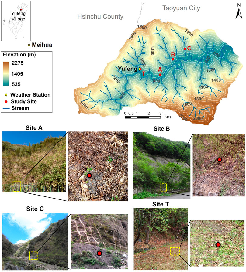
FIGURE 2. A map displays the locations of the study sites in the Yufeng Village of Taiwan and the two nearby weather stations of Yufeng and Meihua. The study sites A, B, and C are situated in landslide active areas, where site T is in a flat grassland in the Yufeng Elementary School.

The study sites A, B, and C are selected at a reachable hillslope adjacent to roads, so we can evaluate the landslide risks to the residents by assessing the soil moisture condition to the occurrence of landslide. These sites have had landslide incidents in recent 10 years (Figure 2). These sites are all situated at hills composed of hardly weathered lithosols with the slopes larger than 20° (Chen et al., 2010). The site T, situated in a flat grassland in the Yufeng Elementary School, is selected to test the model’s applicability in different soil profiles and settings (Figure 2). We sampled the in-situ soil moisture content at sites A, B, C, and T once a month. The measurements were taken by FieldScout^® time-domain reflectometry (TDR) 350, a commonly used volumetric water content device, at specific depths determined by the length of the rods. Due to the hardness of the soils at sites, measurements could only be obtained at depths of 200 mm at site A, 76 mm at site B, 120 mm at site C, and 120 mm at site T.

To implement the model, we assemble hourly meteorological data provided by the Water Resources Agency and Central Weather Bureau, including precipitation (P), mean air temperature (T_a), daily minimum air temperature (T_min), daily maximum air temperature (T_max), wind speed ($u$), and atmospheric pressure (P_r) from the two nearby weather stations of Yufeng and Meihua (Figure 2). To examine the physical soil properties (i.e., the percentage of sand, silt, clay, bulk density, and depth of soil horizons) at sites A, B, and C, we employ the SoilGrids 2.0 system (https://soilgrids.org), a digital soil mapping on soil properties and classes using global covariates and globally fitted models at a spatial resolution of 250 m (Poggio et al., 2021). The physical soil properties at site T was sampled using the Bouyoucos-hydrometer method.

Major hydrological fluxes, including I, q_H, q_p, q_s, and ET, are depicted by the differences between the saturated and unsaturated conditions at layer ij. In this research, i was set to the classification types determined by the SoilGrids 2.0 at sites A, B, and C or by the lab experiment at site T, and j was set to 10, to estimate the associated dynamic water movement within different soil layers (Figure 1). The soil moisture content (${\theta }_i^j$) was simulated from the land surface to the soil layer in compliance with the rod length used at each site, and transformed into the volumetric soil water content (${\theta }_i^{\ast j}$) by the thickness of each layer. In order to compare our model predictions with the field measurements, we further calculated θ^* by averaging the simulated ${\theta }_i^{\ast j}$, because the value provided by TDR 350 measurements was the average of the soil moisture content across the rod length. In addition, to catch the rapid change of the shallow soil water content and the associated hydrological processes, the simulation time interval was set to 1 h with a time step of 1/60, of which it executes 60 simulations per time interval.

3.2 Model calibration/validation and sensitivity analysis

We calibrate the model parameters of ${\theta }_s^{\ast }$, ${\theta }_f^{\ast }$, ${\theta }_r^{\ast }$, and ${\theta }_w^{\ast }$, and the PTFs coefficients using the Monte-Carlo method ranging from a lower bound of 10% to an upper bound of 10 times the documented values from the literature. After calibration, we validate the model performance by comparing model predictions for a given set of conditions using input parameters measured or determined during the calibration process with the in-situ measurements of the soil moisture content (Moriasi et al., 2007). Model performance is quantified by indicators of mean error (ME), mean absolute error (MAE), and root mean square error (RMSE).

To evaluate the meteorological effects on the related hydrological processes under the hypothetical climate change perturbations, we perform a sensitivity analysis at site B. The local perturbation method (Haan, 2002; Cheng and Wiley, 2016) is applied. We independently manipulated the magnitude of P and T_a by changing one parameter at a time holding all others constant with a fraction of $f_i$ from the baseline condition (McCuen, 2002; Cheng and Wiley, 2016). The sensitivity (S) was calculated using the following equations (van Griensven et al., 2006):

${\mathit{S}}_{\mathit{P}}=\frac{\mathit{M}\left(\mathit{P}\cdot {\mathit{f}}_{\mathit{i}}\right)-\mathit{M}\left(\mathit{P}\right)}{\mathit{M}\left(\mathit{P}\right)},(42)$

${\mathit{S}}_{{\mathit{T}}_{\mathit{a}}}=\frac{\mathit{M}\left({\mathit{T}}_{\mathit{a}}+{\mathit{f}}_{\mathit{i}}\right)-\mathit{M}\left({\mathit{T}}_{\mathit{a}}\right)}{\mathit{M}\left({\mathit{T}}_{\mathit{a}}\right)},(43)$

where $S_P$ and $S_{T_a}$ are the sensitivities to the variable of P or T_a, M(P) and M(T_a) are the model simulations using the observed hourly precipitation (P) or the hourly air temperature measurements (T_a), and $f_i$ is the fraction being used to adjust the model inputs. To produce the perturbation in precipitation, we adjust the value of P by multiplying the factor of $f_i$ from 0.2 to 2, where the observed P is set as $f_i=1$. The perturbation in air temperature (T_a) is produced by adding the factor of $f_i$ independently from −4 to 5°C, where the observation T_a. is set as $f_i=0$. The simulated results based on the observed weather conditions (i.e., M (P) and M (T_a)) are used as baselines. $M\left(P\cdot f_i\right)$ and $M\left(T_a+f_i\right)$ refer to the model predictions to the corresponding fractional changes in $P$, and the magnitude change in $T_a$ with the defined $f_i$, respectively. The range of the perturbations is determined according to the predictions of precipitation and air temperature by Taiwan Climate Change Projection Information and Adaption Knowledge Platform (TCCIP) under the worst climate change scenario of RCP 8.5 (IPCC, 2017). The analyses are classified into four periods, namely January to March, April to June, July to September, and October to December.

4 Results

4.1 Simulated results and model performance

Based on the soil property information (Table 1), we parameterized the associated soil hydraulic parameters used in the PTFs and the saturated hydraulic conductivity (Table 2) to simulate hourly soil moisture dynamics in 2019. To evaluate model performance, we compared the simulated volumetric soil water content (θ^*) to the in-situ measurements by TDR 350 at sites A, B, C, and T. In Figure 3, we present the simulation results used for model calibration from 2019/1/1 to 2019/7/31 and the model performance determined by a model validation test from 2019/8/1 to 2019/12/31. The simulated results of the volumetric soil water content showed wide ranges at sites A, B, C, and T, from 4.0 to 23.5%, 4.2–17.3%, 2.8– 34.0%, and 2.7–45.3%, respectively. These values were generally followed the in-situ measurements at the same sites ranged from 2.3 to 10.6%, 1.6–14.9%, 2.9–20.3%, and 10.9–35.4%, respectively. However, larger discrepancies were noticed at sites C and T. During severe rainfall events and dry periods, the model underestimated the volumetric soil water contents (Figure 3). Based on the statistical error indices, model performance at sites A, B, C, and T was evaluated as ME: −0.67, 0.53, −5.46, and −5.39; MAE: 1.40, 1.25, 5.46, and 6.47; and RMSE: 1.92, 1.44, 7.27, and 7.98, respectively.

TABLE 1

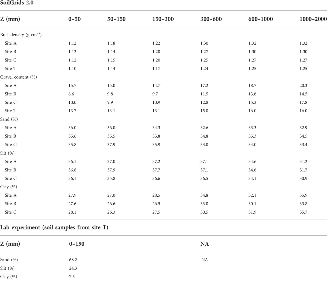
TABLE 1. The soil properties at sites A, B, C, and T from methods of SoilGrids 2.0 and lab experiment.

TABLE 2

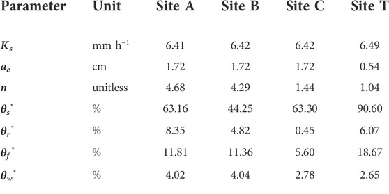
TABLE 2. Parameterization results at sites A, B, C, and T, were calculated by PTFs based on their specific soil properties.

FIGURE 3

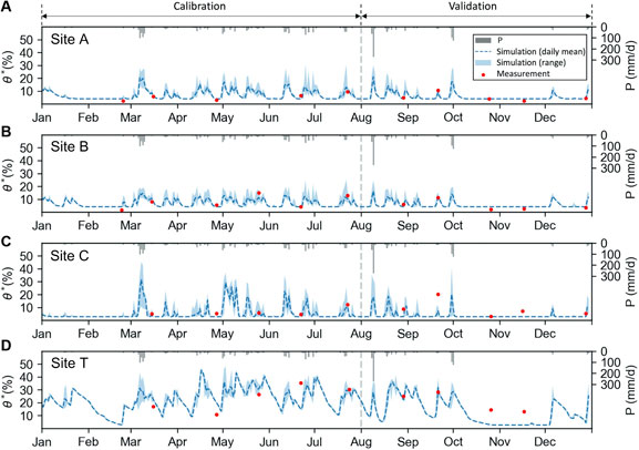
FIGURE 3. The in-situ measurements and the simulation results of the volumetric soil water content (θ^*) at (A) site A, (B) site B, (C) site C, and (D) site T in the Yufeng watershed.

4.2 The monthly hydrological variations

The hourly simulation results were accumulated into a monthly time scheme from 2019/01-2019/12 to present the monthly hydrological variations (Figure 4). We found that the patterns of infiltration (I) and percolation (q_p) at sites A, B, and C followed the pattern of monthly precipitation closely. Since the infiltration capacity of soil (I_c) was greater than the precipitation at these sites, the magnitude of the infiltration was set to the value of precipitation (i.e., I = P). In 2019, the highest infiltration (I) occurred in August due to typhoons. The percolation (q_p) at sites A, B, and C had the highest value of 376, 368, and 254 mm in August, respectively, and the lowest nearly 0 mm in February and November. The infiltration and percolation were generally high during the wet seasons, such as the monsoon season in May and June, and the typhoon season in August. During the dry season in the winter time, the infiltration and percolation were relatively low. Comparatively, the percolation (q_p) at site T was at a very low magnitude around 0 mm in most of the months, except in March, August, and October. The highest monthly evapotranspiration (ET) was around 220 mm at site C in May, while the lowest ET was around 2 mm in November. Comparing to site C, ET at sites A and B ranged from 2 mm in November to 150 mm in May. In contrast, site T had the lowest ET, spanning from 2 mm in November to 91 mm in May. The changes in soil moisture content (Δθ) reflected the net changes from the associated hydrological components of P, I, q_p, and ET with seasonal characteristics. The accumulative soil moisture content in a month (θ, mm) was lower at sites A and C than at sites B and T. When we transformed the soil moisture content (θ, mm) into the volumetric soil water content (θ^*, %), sites A, B, and C, had similar magnitude of θ^*. At sites A, B, and C, θ^* was around 2.8–11.6% and varied slightly throughout the year, while θ^* appeared greater variations at site T from the lowest around 2.7% in November to the highest around 32.7% in May.

FIGURE 4

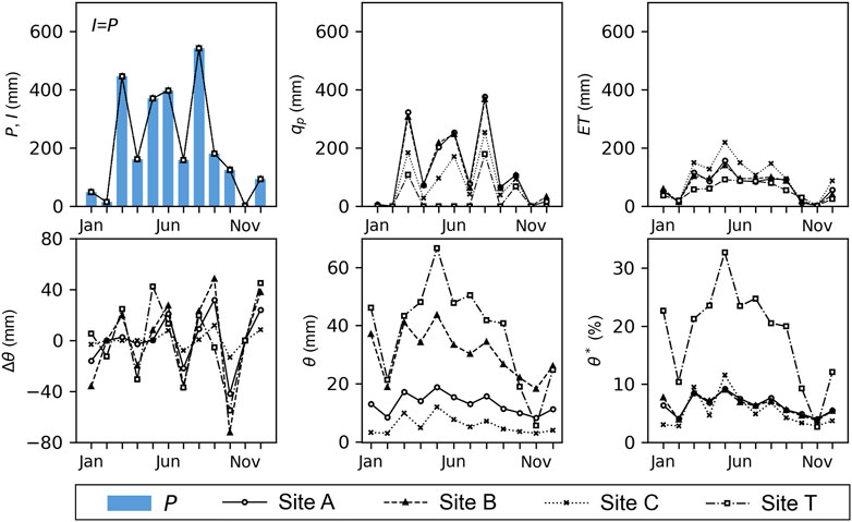
FIGURE 4. Simulation results of the main hydrological processes were summarized into monthly averages of I, q_p, ET, Δθ, θ, and θ^* at sites A, B, C, and T.

4.3 Sensitivity to precipitation and air temperature

The sensitivity results demonstrated that seasonal responses of hydrological processes were complex resulting in nonlinear responses of θ^* and ET, and a more linear influence on $q_p$ with regard to the baseline characteristics of P. In contrast, changes in the hydrological processes of θ^*, q_p, and ET to T_a were more linear in comparison to P (Figures 5, 6).

FIGURE 5

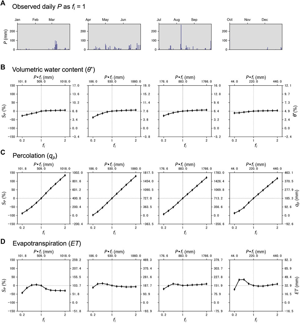
FIGURE 5. Based on (A) the observed daily accumulated precipitation as f_i = 1, we present the sensitivity analysis results of (B) soil moisture content (θ^*), (C) percolation (q_p), and (D) evapotranspiration (ET) in four periods-- January to March, April to June, July to September, and October to December. In Figures 5B–D, the lower x-axis denotes the fractional change (f_i), and the upper x-axis represents the range of P in the sensitivity analysis. The left y-axis represents the sensitivity to precipitation (S_p), while the right y-axis indicates the simulated results of the magnitude of the correspondent hydrological process.

FIGURE 6

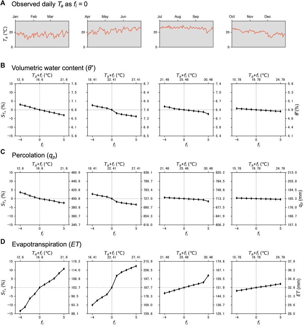
FIGURE 6. Based on (A) the observed daily mean air temperature as f_i = 0, we present the sensitivity analysis results of (B) soil moisture content (θ^*), (C) percolation (q_p), and (D) evapotranspiration (ET) in four periods-- January to March, April to June, July to September, and October to December. In Figures 6B–D, the lower x-axis denotes the fractional change (f_i), and the upper x-axis represents the range of T_a in the sensitivity analysis. The left y-axis represents the sensitivity to air temperature (S_Ta), while the right y-axis indicates the simulated results of the magnitude of the correspondent hydrological process.

To better depict the trend, we compared the rate of change among different seasons. With prolonged rainfall events from April to September, the fractional change in precipitation (P) with $f_i>1$ was found to result in a slight increase of θ^*. Yet, from October to December the response of θ^* to the fractional change of P ($f_i>1$) was minimal due to very little precipitation occurring in the period. In contrast, the fractional change in precipitation with $f_i<1$ was found to cause a greater drop of θ^* from January to September than that from October to December, which may be attributed to the differences in the frequency and intensity of the baseline precipitation condition (Figures 5A,B).

The sensitivity of q_p to changes in P was much larger than that of θ^* among seasons. We observed that S_P reached about 150% with a fractional change in P at $f_i=2$ (Figure 5C). An interestingly divergent behavior was found in ET that it displayed nonlinear responses to changes in P. With changes in P at $f_i<1$, reactions of ET appeared as a hyperbolic curve that the direction turned from a positive sensitivity to a negative one at different fractions among seasons. Nonetheless, with changes in P at $f_i>1$, increases in P caused different reactions of ET. From January to June, the rate of change was negative, while from July to December, it was positive (Figure 5D).

In terms of the change in T_a, the sensitivity results showed that θ^* and q_p both reacted negatively to changes in T_a (Figure 6). The sensitivity (S_Ta) was about 3–4% with a 5°C increase, or a 4°C drop in T_a (Figures 6B,C). In addition, a larger sensitivity was depicted on q_p from January to June, than that from October to December (Figure 6C). ET was found to be the most sensitive hydrological process to temperature (Figure 6D). Nonlinear reactions were seen from January to March, and from April to June, while more linear reactions were found from October to December. Besides, larger positive sensitivity was also found from January to March, and from April to June. Yet, it was less sensitive to changes in T_a from October to December (Figure 6D). In sum, we concluded that q_p was the most sensitive hydrological process to the variation of P (Figure 5C), while ET possessed the highest sensitivities to changes in T_a (Figure 6D). According to these results, the influence of precipitation or temperature on different hydrological processes vary depending on the seasonal meteorological patterns.

5 Discussion

The shallow soil moisture determines the onset of landslide occurrence and is critical for agricultural production in mountainous landslide-active regions. However, predicting the rapid change of the shallow soil moisture content and the associated hydrological processes is challenging due to the severe lack of in-situ measurements of soil moisture content. Our model coupled classic continuity equations to estimate various processes in the soil column. Based on the well-known physics equations and the associated processes, the model was designed particularly for sites lacking sufficient monitoring data. To overcome the shortage of field data, we simplified several complex parameterizations seen in most distributed models without sacrificing the ability for short-time predictions. The model was proved to provide reasonably well predictions of the vertical soil moisture content and the associated hydrological processes of infiltration, evapotranspiration, percolation, and surface runoff in a short time scheme. Given the spatial information of the physical soil properties provided by SoilGrids 2.0, the model can be used to predict the spatial distribution of soil moisture content in different meteorological conditions. The comprehensive information can be linked with the mapping of landslide-prone areas to support the detection of the early warning signals in landslide-active regions and examine the effects of climate change.

5.1 General perspective from the modeling results

Results showed that the model provides reasonably good predictions of the soil moisture contents and gives insights into how the vertical soil properties and climatic variations influence the dynamics of water movement. Given the interlinkage of each hydrological process by mathematical equations in the model, the hydrological changes can be partitioned. Different soil properties, particularly the soil texture and the formation structure, have been used to determine the porosity affecting the interrelated soil moisture content of θ_s, θ_f, θ_w, and θ_r. Based on SoilGrids 2.0, the soil moisture content was found to be influenced majorly by the formation of the soil structure (Poggio et al., 2021), with the marginal differences contributed to the correspondent soil texture and the coarse fragments (Domínguez-Niño et al., 2020). This is especially evident at site T, where the simulation results showed a generally higher soil moisture content than the other three sites across the one-year simulation period. The topsoil in site T was designed and made for grassland that supports higher field water content (θ_f) and lower percolation (q_p). This was very dissimilar from the soils in the landslide active areas that were naturally composed of poorly developed and hardly weathered lithosols (Chen et al., 2010). The presence of these coarse particles and the hardly weathered soil were found to induce appreciable variabilities to higher permeability, and in turn, result in lower soil water content (Chow et al., 2007; García-Gamero et al., 2021).

Besides the soil properties, seasonal variations in the meteorological conditions were found to cause great hydrological variations across a year. Under heavy rainfall conditions in geologically unstable areas such as sites A, B, and C, the effects of soil suction due to the fast response of θ to a rapid increase in precipitation, are closely related to the probability of landslide occurrence (Ray et al., 2010). This information is particularly important in the development of landslide early warning system for the security of the tribe community in Yufeng to avoid dreadful disasters. Model predictions on q_p and ET are additional supporting information for environmental planning and watershed management. This information provides critical scientific foundation on the strength of the natural hydrological processes in reducing the susceptibility to sliding and slope failure. For example, the magnitude of ET is highly related to soil suction levels or slope angles exceeding friction angles, whereas q_p is in charge of regulating and removing water underground, which can help stabilize hillslopes (Reder et al., 2018; Sidle et al., 2019).

During droughts, on the other hand, predictions of shallow soil moisture content are critical for agricultural production (Fan et al., 2022). In Yufeng, dry seasons account for about 6 months in a year. With this shallow soil moisture model cooperating with no or little precipitation weather forecasts, it can help provide predictions on where and for how long situations of water shortage will occur and assist tribe people to adapt in advance for crop types and agricultural operations.

5.2 Comparison to the existing approaches

Given the quick response of water movements in the landslide areas, the landslide research often requires detection of the land surface process in a short time scheme (Matsuura et al., 2008). Our model provides dynamic predictions on water movements in soils accounting for the influence of the meteorological forcing and the vertical soil heterogeneity (Lu et al., 2020). They are vital supporting information in detecting the early warning signals in the landslide-active regions when linking with the mapping of the landslide-prone areas. In searching of the existing models, such as SWAT (Soil Water Assessment Tool; Arnold et al., 2012), SpaFHy (Spatial Forest Hydrology model; Launiainen et al., 2019), GIPL2 (Geophysical Institute Permafrost Lab version 2, Qin et al., 2017), their simulation time scales are often limited at a daily time scheme not able to capture the rapid variations of the soil moisture in the landslide areas. To estimate the rapid vertical hydrological processes in the soil column, our model was designed particularly for sites lacking sufficient monitoring data to accomplish the complex parameterizations. We made simplifying assumptions to overcome the shortage of field data, and applied the well-known physics equations coupling the heterogeneous vertical soil physical properties obtained from the SoilGrids 2.0 to produce relatively accurate estimates of the vertical soil moisture dynamics and the associated hydrological processes. Moreover, with the advances of the satellite-based approaches in extracting multiple spatial information, it facillitates progress in modeling and landslide research. In recent years, many distributed models have benefited from the satellited-based approaches to derive coarse-scale spatial attributes of land use types, soil profiles, and water fluxes (Li et al., 2019; Fisher and Koven, 2020; Senent-Aparicio et al., 2020; Rouf et al., 2021). For example, Rouf et al. (2021) took the hyper-resolution forcing data from the satellite-based observations into land surface models to estimate the soil moisture contents at the resolution of 500 m. The soil profile data used in our model were provided by SoilGrid 2.0, which assembled the satellite-derived information in climatic, global landform, and lithology with the machine-learning techniques by a big database of the global soil profiles to produce the global digital soil map at a resolution of 250 m (Hengl et al., 2017; Poggio et al., 2021). Therefore, if spatially-distributed information is available, such as the meteorological conditions and the vertical soil profiles, our model has the potential to expend into a spatially distributed model in predicting the vertical soil moisture content as well as the associated hydrological processes.

5.3 Implications from sensitivity analyses

Facing great threats from the increasing air temperature and changes in the frequency and intensity of precipitation, more attention has been focused on monitoring the soil moisture content and the associated hydrological processes for their critical characteristics to the incidence of many severe damages, such as debris flow, landslide, soil erosion, and agricultural loss. Based on the sensitivity analysis results, we clarified the influence of P and T_a on shallow soil moisture content and other associated hydrological processes. In general, θ^* and q_p both increase with P, and decrease with T_a. In contrast, ET increases with T_a, but responses of ET to P are very nonlinear, depending upon the magnitude and pattern of P (Bao et al., 2012). Insights from the sensitivity results suggest higher impacts on q_p, followed by ET and θ^*, when changes in P are higher than T_a. On the contrary, if a larger change of T_a is happening, greater variations will be found in ET, followed by θ^* and q_p. The hydrological processes are frequently associated with disasters. For example, soil erosion is often related to the aggregation of soil moisture (Cotler and Ortega-Larrocea, 2006), and percolation is one of the processes that trigger shallow landslides no more than 1–2 m.

In addition to the influence of meteorological factors, the interactions between different hydrological processes also play parts of the governing role in the physical mechanisms of hydrological cycling. To better clarify the interactions, we sketch the contours of the water balance by a feedback loop (Koster et al., 2003), that outlines the interactions between P, θ, and ET. In the loop, precipitation will increase the soil moisture, and in turn, the wet soil will contribute to higher ET, which will provide abundant vapor as positive feedback to the formation of precipitation. This is the so-called θ-P feedback loop (Yang et al., 2018). Built upon the viewpoints gained from the sensitivity results, a more detailed θ-P feedback loop can be sketched for different states of each element to outline the land-atmosphere causal relationship under various environmental and meteorological conditions (Figure 7). Starting from the element of precipitation, no matter small or large P will boost up θ. Nonetheless, the condition of the ground will give a different path to ET. If the ground is very dry, the increase of θ will cause ET to increase. In contrast, when the ground is wet to the maximum field capacity, ET decreases when θ increases. The status of ET will determine the enhancement or breakdown of P (Figure 7).

FIGURE 7

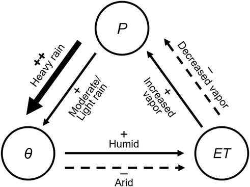
FIGURE 7. Detailed $\theta$-P feedback loop built from the sensitivity results.

5.4 Possible sources of uncertainty

The inability of this modeling approach in detecting the targeted hydrological processes may come from possible sources of observation uncertainty, process uncertainty, and model uncertainty (Francis and Shotton, 1997). The aware uncertainties are the tradeoffs we made between the model accuracy, cost, and time. The first possible uncertainty may arise from the observation uncertainty used to run the model due to inconsistencies in the measurement technique (precision) and/or the measurement bias (accuracy) of the soil moisture data and meteorological information. As the in-situ measurements of the soil moisture content were taken by FieldScout^® TDR 350, the setup of this volumetric device would unavoidably cause a certain loss of the measurements to the true value of the soil moisture content, and produce measurement errors. Moreover, lacking a continuous monitoring device, the measurements of the soil moisture content were limited to once a month, and due to safety concerns for conducting field surveys in landslide-active areas, most measurements of the soil moisture content were taken on non-raining days. Consequently, the limited data on soil moisture content may constrain the extent for calibration. The other possible observation uncertainty may come from the meteorological data. Although we took the information from most nearby weather stations, in mountainous areas, topography could cause variations in the micro-climates even within a short distance, especially the precipitation. The other possible influence of topography on the model accuracy can result from the ignorance of the lateral flow in uneven terrains. According to the in-situ slope measurements, the slopes of sites A, B, C, and T were 36.7°, 40.7°, 20.3°, and 0°, respectively. Based on the model performance, we found that model simulations had smaller errors at sites A and B than at sites C and T. However, sites A and B were situated at hills with steeper slopes than sites C and T. This also demonstrated that predicting soil moisture based on the simplified assumption considering only one-dimensional movements dominant by gravity forces, the potential errors were minor for high-slope landslide terrains. In addition, the soil properties are the inherent factor to define the boundary of matric potential and the hydraulic conductivity that regulates the variations of the soil moisture content (Qi et al., 2018). The physical properties of the soil were described by PTFs from the SoilGrids 2.0 without validation. As the precipitation and soil properties are major input variables to define the source of water and boundary of the variations in soil moisture content, under the theory of water balance, uncertainties from these discrepancies to the reality are expected.

Second, the association of the inherent stochasticity and natural variability of system components may cause extrinsic process uncertainty to be modeled (Hilborn and Mangel, 2013). The process uncertainty in this research could have arisen from the setup of the time step of the simulation. For example, since soil moisture content can be highly variable within shallow soil depth in space and time, saturation during rainfall events or soil moisture content reaching wilting point during droughts may occur in a very short time (Qi et al., 2018). Currently, the finest simulation time step was set to 1 minute to compute the prompt responses to heavy rain or drought conditions. Nonetheless, the simulation requires high computing equipment and is very time-consuming. If a process uncertainty exists for this setup, over- or under-estimating the shallow soil moisture content is unavoidable.

The third source of the uncertainty may be related to the selection of mathematical equations that can accurately describe the water movement as the numerical solution in the model. In the water cycling system, the associated hydrological processes are highly complicated both above and beneath the soil surface. Most processes involve nonlinearities and hysteresis in space and time, so model uncertainty may present in any estimation of the water fluxes (van Dam and Feddes, 2000), such as the percolation flux using the Richards equation, the spatial variability of plant interception, and the coarse fragments accounted for surface or subsurface water dynamics (He et al., 2014; Ogden et al., 2015).

Lastly, the model uncertainty may come from the simplified assumption of the underground movement of the soil water going downward without lateral flow. This simplification was made based on the geological environment in Yufeng, consisting of sandy shale lithosol (90.82%) and sandy shale darkish colluvial soils (9.18%). It gives high water conductivity in the study sites so that the gravitational flow can be considered the dominant process to ignore the lateral flow. However, we cannot deny that the multifaceted topographical surface will redistribute some lateral water movements, which was not considered in the model (Chen et al., 2014). As a result, the unknown pores may increase the curvature of water flow and result in preferential flow and infiltration redistribution.

5.5 Potential applications

Climate change has created challenges for decision-makers (Abbaspour et al., 2015). The Food and Agriculture Organization (FAO) forecasted problems in agriculture (FAO, 1983). The flooding issues bring excessive surface runoff that will damage the crops, while severe droughts create water deficit problems that will impede crop growth. The fundamental scientific basis of the soil moisture dynamics and the critical hydrological processes is in pressing need for decision-makers to prepare for the potential impacts of climate change (Nyamgerel et al., 2022; Tan et al., 2022).

The simulation results from this research provide valuable indications in hourly, daily, monthly, and seasonally for use in different purposes of natural resources management. For example, modeling the strength of ET, θ, and q_p, can be used to detect water stress as water scarcity indicators or drought indices (Sohrabi et al., 2015), because they are linked to capturing variations of precipitation, temperature, and water cycling over time to characterize the availability of water. The interlinkage of the hydrological processes, as we have shown in the detailed θ-P feedback loop, can help monitor drought evolution (Teuling et al., 2013). The model predictions of soil moisture content under different weather conditions and soil types can be used for agricultural planning, erosion control, or hazard management.

Furthermore, this dynamic modeling approach can account for the continuity of month-to-month transitions to obtain various predictions of θ, θ_f, θ_w, q_H, q_s, and ET, and helps characterize droughts/flooding for crop health management and determine impacts under dry/wet conditions. For disaster-related applications, infiltration and surface runoff predictions can be used to understand the extent of erosion on hillslopes (Nearing et al., 1989). For example, a lot of evidence worldwide suggest that areas previously occurred landslides would have a higher probability to reoccur in the future (Temme et al., 2020). The variations of soil moisture in the unsaturated zone of the landslide-prone areas have been applied to determine the wetness index and the safety factor of the slope instability in the landslide instability models (Ray et al., 2010). Based on the simulation results, it showed that in the landslide active regions, soil moisture may be relatively low compared to sites with different soil properties, but the response to precipitation was rapid due to relatively high slopes and unique soil properties and the fragile geological structures in landslide active regions. These effects were modeled in this study to help detect the changes in the hydrological processes underneath the ground. This is why soil hydrology has become a weight-bearing point providing designing emphasis on structure safety to prevent shallow landslides and control slope stability (Ray et al., 2010; Bittelli et al., 2012). Possible mitigation and adaptation strategies for land governance should be planned in response to future climate situations (Tan et al., 2022), such as early actions on constructing drainage tunnels, gutters, or ditches to reduce the risks of landslides (Lahmer, 2003; Sun et al., 2010), and preparation on backup planning for irrigation or domestic purposes.

6 Conclusion

The shallow soil moisture dynamics play a crucial role in regulating water balance and are critical information for disaster management and agricultural practices. In this paper, we present a newly constructed system dynamics soil moisture model based on the law of water balance and the physical mechanisms of the interlinked hydrological processes. We calibrated and validated simulation results of the shallow soil moisture content in the Yufeng Village, a landslide-prone region and a traditional tribe settlement area. Our simulated results showed good fits with the in-situ measurements. The model can be applied to predict the associated hydrological processes and provide information for agricultural planning and disaster prevention. In addition, results from the sensitivity analyses revealed the potential impacts of climate change. We sketched a detailed feedback loop of the water cycling associated with precipitation, soil moisture, and evapotranspiration. With the general structure of this physically-based model, we believe this modeling approach can be applicable and transferable to other regions to deliver useful predictions for agricultural applications or disaster management coping with climate change.

Data availability statement

The original contributions presented in the study are included in the article, further inquiries can be directed to the corresponding author.

Author contributions

Material preparation and data analysis were performed by JYD. Funding was acquired by STC. JYD and STC both contributed to model construction, manuscript writing, and interpretation of the results.

Funding

This work was funded by Ministry of Science and Technology, Taiwan, R.O.C. (project number: MOST 106-2621-M-002-011-MY2 & MOST 108-2621-M-002-010-MY3), and National Taiwan University (project title: Evaluating resilience of water resources by a system dynamics modelling approach; project billing number: NTU-CC-111L894705).

Acknowledgments

We sincerely thank Chuang-Yuan Kuo, Zih-Yang Wang, and Kai-Chih Yin for their assistance with the field survey and preliminary data collection.

Conflict of interest

The authors declare that the research was conducted in the absence of any commercial or financial relationships that could be construed as a potential conflict of interest.

Publisher’s note

All claims expressed in this article are solely those of the authors and do not necessarily represent those of their affiliated organizations, or those of the publisher, the editors and the reviewers. Any product that may be evaluated in this article, or claim that may be made by its manufacturer, is not guaranteed or endorsed by the publisher.

Reference

Abbaspour, K. C., Rouholahnejad, E., Vaghefi, S., Srinivasan, R., Yang, H., and Kløve, B. (2015). A continental-scale hydrology and water quality model for Europe: Calibration and uncertainty of a high-resolution large-scale SWAT model. J. Hydrol. X. 524, 733–752. doi:10.1016/j.jhydrol.2015.03.027

CrossRef Full Text | Google Scholar

Albright, W. H., Gee, G. W., Wilson, G. V., and Fayer, M. J. (2002). Alternative cover assessment project Phase I Report. Nevada, USA: Desert Research Institute.

Google Scholar

Allen, R. G., Pereira, L. S., Raes, D., and Smith, M. (1998). Crop evapotranspiration-Guidelines for computing crop water requirements-FAO Irrigation and drainage paper 56. Rome: FAO.

Google Scholar

Arampatzis, G. K., Tzimopoulos, C. D., and Evangelides, C. Η. (2011). Numerical solution of Richards' equation with control volume method. J. Mech. Behav. Mat. 15, 291–308. doi:10.1515/jmbm.2004.15.4-5.291

CrossRef Full Text | Google Scholar

Arnold, J. G., Moriasi, D. N., Gassman, P. W., Abbaspour, K. C., White, M. J., Srinivasan, R., et al. (2012). SWAT: Model use, calibration, and validation. Trans. ASABE 55, 1491–1508. doi:10.13031/2013.42256

CrossRef Full Text | Google Scholar

Bao, Z., Zhang, J., Liu, J., Wang, G., Yan, X., Yan, X., et al. (2012). Sensitivity of hydrological variables to climate change in the Haihe River basin, China. Hydrol. Process. 26, 2294–2306. doi:10.1002/hyp.8348

CrossRef Full Text | Google Scholar

Bittelli, M., Valentino, R., Salvatorelli, F., and Rossi Pisa, P. (2012). Monitoring soil-water and displacement conditions leading to landslide occurrence in partially saturated clays. Geomorphology 173-174, 161–173. doi:10.1016/j.geomorph.2012.06.006

CrossRef Full Text | Google Scholar

Brocca, L., Ciabatta, L., Massari, C., Camici, S., and Tarpanelli, A. (2017). Soil moisture for hydrological applications: Open questions and new opportunities. Water 9, 140. doi:10.3390/w9020140

CrossRef Full Text | Google Scholar

Brocca, L., Morbidelli, R., Melone, F., and Moramarco, T. (2007). Soil moisture spatial variability in experimental areas of central Italy. J. Hydrol. X. 333, 356–373. doi:10.1016/j.jhydrol.2006.09.004

CrossRef Full Text | Google Scholar

Cass, A., Campbell, G. S., and Jones, T. L. (1984). Enhancement of thermal water vapor diffusion in soil. Soil Sci. Soc. Am. J. 48, 25–32. doi:10.2136/sssaj1984.03615995004800010005x

CrossRef Full Text | Google Scholar

Chen, C., Hu, K., Ren, T., Liang, Y., and Arthur, E. (2017). A simple method for determining the critical point of the soil water retention curve. Soil Sci. Soc. Am. J. 81, 250–258. doi:10.2136/sssaj2016.06.0187

CrossRef Full Text | Google Scholar

Chen, C. Y., Cheng, L. K., Yu, F. C., Lin, S. C., Lin, Y. C., Lee, C. L., et al. (2010). Landslides affecting sedimentary characteristics of reservoir basin. Environ. Earth Sci. 59, 1693–1702. doi:10.1007/s12665-009-0151-0

CrossRef Full Text | Google Scholar

Chen, M., Willgoose, G. R., and Saco, P. M. (2014). Spatial prediction of temporal soil moisture dynamics using HYDRUS-1D. Hydrol. Process. 28, 171–185. doi:10.1002/hyp.9518

CrossRef Full Text | Google Scholar

Chen, Q. G. (1983). Soil of slopeland in Hsinchu. Nantou: Mountain Agricultural Resources Development Bureau.

Google Scholar

Cheng, S. T., and Wiley, M. J. (2016). A reduced parameter stream temperature model (RPSTM) for basin-wide simulations. Environ. Model. Softw. 82, 295–307. doi:10.1016/j.envsoft.2016.04.015

CrossRef Full Text | Google Scholar

Chow, T., Rees, H., Monteith, J., Toner, P., and Lavoie, J. (2007). Effects of coarse fragment content on soil physical properties, soil erosion and potato production. Can. J. Soil Sci. 87, 565–577. doi:10.4141/CJSS07006

CrossRef Full Text | Google Scholar

Clark, M. P., Nijssen, B., Lundquist, J. D., Kavetski, D., Rupp, D. E., Woods, R. A., et al. (2015). A unified approach for process‐based hydrologic modeling: 2. Model implementation and case studies. Water Resour. Res. 51, 2515–2542. doi:10.1002/2015WR017200

CrossRef Full Text | Google Scholar

Cotler, H., and Ortega-Larrocea, M. P. (2006). Effects of land use on soil erosion in a tropical dry forest ecosystem, Chamela watershed, Mexico. Catena 65, 107–117. doi:10.1016/j.catena.2005.11.004

CrossRef Full Text | Google Scholar

Darcy, H. (1856). Les fontaines publiques de la ville de Dijon: Exposition et application des principes à suivre et des formules à employer dans les questions de distribution d'eau. Paris: Victor Dalmont.

Google Scholar

Deshmukh, A., and Singh, R. (2016). Physio-climatic controls on vulnerability of watersheds to climate and land use change across the U. S. Water Resour. Res. 52, 8775–8793. doi:10.1002/2016WR019189

CrossRef Full Text | Google Scholar

Devia, G. K., Ganasri, B. P., and Dwarakish, G. S. (2015). A review on hydrological models. Aquat. Procedia 4, 1001–1007. doi:10.1016/j.aqpro.2015.02.126

CrossRef Full Text | Google Scholar

Domínguez-Niño, J. M., Arbar, G., Raij-Hoffman, I., Kisekka, I., Girona, J., and Casadesús, J. (2020). Parameterization of soil hydraulic parameters for HYDRUS-3D simulation of soil water dynamics in a drip-irrigated orchard. Water 12, 1858. doi:10.3390/w12071858

CrossRef Full Text | Google Scholar

Fan, J., Han, Q., Tan, S., and Li, J. (2022). Evaluation of six satellite-based soil moisture products based on in situ measurements in Hunan Province, Central China. Front. Environ. Sci. 10, 829046. doi:10.3389/fenvs.2022.829046

CrossRef Full Text | Google Scholar

Fan, J., McConkey, B., Janzen, H., and Wang, H. (2016). Root distribution by depth for temperate agricultural crops. Field Crops Res. 189, 68–74. doi:10.1016/j.fcr.2016.02.013

CrossRef Full Text | Google Scholar

FAO (1983). Guidelines: Land evaluation for Rainfed Agriculture. Rome: FAO Soils Bulletin, 52.

Google Scholar

Fayer, M. J. (2000). UNSAT-H version 3.0: Unsaturated soil water and heat flow model: Theory, user manual, and examples. Richland, WA: Pacific Northwest National Laboratory. doi:10.2172/15001068

CrossRef Full Text | Google Scholar

Fick, A. (1855). Ueber diffusion. Ann. Phys. Chem. 170 (1), 59–86. doi:10.1002/andp.18551700105

CrossRef Full Text | Google Scholar

Fisher, R. A., and Koven, C. D. (2020). Perspectives on the future of land surface models and the challenges of representing complex terrestrial systems. J. Adv. Model. Earth Syst. 12, e2018MS001453. doi:10.1029/2018MS001453

CrossRef Full Text | Google Scholar

Francis, R., and Shotton, R. (1997). Risk” in fisheries management: A review. Can. J. Fish. Aquat. Sci. 54, 1699–1715. doi:10.1139/f97-100

CrossRef Full Text | Google Scholar

Fredlund, D. G., and Xing, A. (1994). Equations for the soil-water characteristic curve. Can. Geotech. J. 31, 521–532. doi:10.1139/t94-061

CrossRef Full Text | Google Scholar

García-Gamero, V., Peña, A., Laguna, A. M., Giráldez, J. V., and Vanwalleghem, T. (2021). Factors controlling the asymmetry of soil moisture and vegetation dynamics in a hilly Mediterranean catchment. J. Hydrol. X. 598, 126207. doi:10.1016/j.jhydrol.2021.126207

CrossRef Full Text | Google Scholar

Glavan, M., and Pintar, M. (2012). “Strengths, weaknesses, opportunities and threats of catchment modelling with Soil and Water Assessment Tool (SWAT) model,” in Water resources management and modeling. Editor P. Nayak (London: InTech). Available from: http://www.intechopen.com/books/water-resources-management-and-modeling/strengths-weaknesses-opportunities-and-threats-of-catchment-modelling-with-soil-and-water-assessment.

CrossRef Full Text | Google Scholar

Haan, C. T. (2002). Statistical methods in hydrology. 2nd ed. Ames, Iowa: Iowa State Press.

Google Scholar

Hassan, G. E., Youssef, M. E., Mohamed, Z. E., Ali, M. A., and Hanafy, A. A. (2016). New temperature-based models for predicting global solar radiation. Appl. Energy 179, 437–450. doi:10.1016/j.apenergy.2016.07.006

CrossRef Full Text | Google Scholar

Haverkamp, R., Debionne, S., Angulo-Jaramillo, R., and de Condappa, D. (2016). “Soil properties and moisture movement in the unsaturated zone,” in The handbook of groundwater engineering. 3rd ed. (Boca Raton, FL: CRC Press), 149–190.

Google Scholar

He, Z. B., Yang, J. J., Du, J., Zhao, W. Z., Liu, H., and Chang, X. X. (2014). Spatial variability of canopy interception in a spruce forest of the semiarid mountain regions of China. Agric. For. Meteorol. 188, 58–63. doi:10.1016/j.agrformet.2013.12.008

CrossRef Full Text | Google Scholar

Hengl, T., de Jesus, J. M., Heuvelink, G. B. M., Gonzalez, M. R., Kilibarda, M., Blagotic, A., et al. (2017). SoilGrids250m: Global gridded soil information based on machine learning. Plos One 12 (2), e0169748. doi:10.1371/journal.pone.0169748

PubMed Abstract | CrossRef Full Text | Google Scholar

Hilborn, R., and Mangel, M. (2013). The ecological detective: Confronting models with data (MPB-28). Princeton, NJ: Princeton University Press. doi:10.1515/9781400847310

CrossRef Full Text | Google Scholar

Horton, R. E. (1940). An approach toward a physical interpretation of infiltration-capacity. Soil Sci. Soc. Am. J. 5, 399–417. doi:10.2136/sssaj1941.036159950005000c0075x

CrossRef Full Text | Google Scholar

IPCC (2014). Climate change 2014: Impacts, adaptation and vulnerability. Part A: Global and sectoral aspects. Cambridge: Cambridge University Press. doi:10.1017/CBO9781107415379

CrossRef Full Text | Google Scholar

IPCC (2017). IPCC fifth assessment report (AR5) observed climate change impacts database, version 2.01. NASA socioeconomic data and applications center (SEDAC). Palisades, NY.

Google Scholar

Jabbar, F. K., and Grote, K. (2020). Evaluation of the predictive reliability of a new watershed health assessment method using the SWAT model. Environ. Monit. Assess. 192, 224. doi:10.1007/s10661-020-8182-9

PubMed Abstract | CrossRef Full Text | Google Scholar

Kanzari, S., Nouna, B. B., Mariem, S. B., and Rezig, M. (2018). Hydrus-1D model calibration and validation in various field conditions for simulating water flow and salts transport in a semi-arid region of Tunisia. Sustain. Environ. Res. 28, 350–356. doi:10.1016/j.serj.2018.10.001

CrossRef Full Text | Google Scholar

Koster, R. D., Suarez, M. J., Higgins, R. W., and Van den Dool, H. M. (2003). Observational evidence that soil moisture variations affect precipitation. Geophys. Res. Lett. 30, 1241. doi:10.1029/2002GL016571

CrossRef Full Text | Google Scholar

Lahmer, W. (2003). Trend analyses of percolation in the State of Brandenburg and possible impacts of climate change. J. Hydrol. Hydromech. 51, 196–209.

Google Scholar

Lane, L. J., and Nearing, M. A. (1989). USDA-water erosion prediction project: Hillslope profile model documentation. West Lafayette, IN: USDA-ARS, National Soil Erosion Research Laboratory.

Google Scholar

Launiainen, S., Guan, M., Salmivaara, A., and Kieloaho, A. J. (2019). Modeling boreal forest evapotranspiration and water balance at stand and catchment scales: A spatial approach. Hydrol. Earth Syst. Sci. 23, 3457–3480. doi:10.5194/hess-23-3457-2019

CrossRef Full Text | Google Scholar

Lei, S., Daniels, J. L., Bian, Z., and Wainaina, N. (2011). Improved soil temperature modeling. Environ. Earth Sci. 62, 1123–1130. doi:10.1007/s12665-010-0600-9

CrossRef Full Text | Google Scholar

Li, J., Li, X., Lv, N., Yang, Y., Xi, B., Li, M., et al. (2015). Quantitative assessment of groundwater pollution intensity on typical contaminated sites in China using grey relational analysis and numerical simulation. Environ. Earth Sci. 74, 3955–3968. doi:10.1007/s12665-014-3980-4

CrossRef Full Text | Google Scholar

Li, T., Guo, S., An, D., and Nametso, M. (2019). Study on water and salt balance of plateau salt marsh wetland based on time-space watershed analysis. Ecol. Eng. 138, 160–170. doi:10.1016/j.ecoleng.2019.07.027

CrossRef Full Text | Google Scholar

Li, Y., and DeLiberty, T. (2021). Evaluating hourly SWAT streamflow simulations for urbanized and forest watersheds across northwestern Delaware, US. Stoch. Environ. Res. Risk Assess. 35, 1145–1159. doi:10.1007/s00477-020-01904-y

CrossRef Full Text | Google Scholar

Lu, H., Zheng, D., Yang, K., and Yang, F. (2020). Last-decade progress in understanding and modeling the land surface processes on the Tibetan Plateau. Hydrol. Earth Syst. Sci. 24, 5745–5758. doi:10.5194/hess-24-5745-2020

CrossRef Full Text | Google Scholar

Lu, N., and Godt, J. (2008). Infinite slope stability under steady unsaturated seepage conditions. Water Resour. Res. 44. doi:10.1029/2008WR006976

CrossRef Full Text | Google Scholar

Lu, N., Godt, J. W., and Wu, D. T. (2010). A closed-form equation for effective stress in unsaturated soil. Water Resour. Res. 46, W05515. doi:10.1029/2009WR008646

CrossRef Full Text | Google Scholar

Ma, T., Han, L., and Liu, Q. (2021). Retrieving the soil moisture in Bare Farmland areas using a modified Dubois model. Front. Earth Sci. 9, 1216. doi:10.3389/feart.2021.735958

CrossRef Full Text | Google Scholar

Matsuura, S., Asano, S., and Okamoto, T. (2008). Relationship between rain and/or meltwater, pore-water pressure and displacement of a reactivated landslide. Eng. Geol. 101, 49–59. doi:10.1016/j.enggeo.2008.03.007

CrossRef Full Text | Google Scholar

McCuen, R. H. (2002). Modeling hydrologic change: Statistical methods. Boca Raton: CRC Press. doi:10.1201/9781420032192

CrossRef Full Text | Google Scholar

Millington, R. J., and Quirk, J. P. (1961). Permeability of porous solids. Trans. Faraday Soc. 57, 1200–1207. doi:10.1039/TF9615701200

CrossRef Full Text | Google Scholar

Moriasi, D., Arnold, J. G., Van Liew, M. W., Bingner, R. L., Harmel, R. D., and Veith, T. L. (2007). Model evaluation guidelines for systematic quantification of accuracy in watershed simulations. Trans. ASABE 50, 885–900. doi:10.13031/2013.23153

CrossRef Full Text | Google Scholar

Mualem, Y. (1976). A new model for predicting the hydraulic conductivity of unsaturated porous media. Water Resour. Res. 12, 513–522. doi:10.1029/WR012i003p00513

CrossRef Full Text | Google Scholar

Nearing, M. A., Foster, G. R., Lane, L. J., and Finkner, S. C. (1989). A process-based soil erosion model for USDA-water erosion prediction project technology. Trans. ASAE 32, 1587–1593. doi:10.13031/2013.31195

CrossRef Full Text | Google Scholar

Noborio, K., McInnes, K. J., and Heilman, J. L. (1996). Two-dimensional model for water, heat, and solute transport in furrow-irrigated soil: II. Field evaluation. Soil Sci. Soc. Am. J. 60, 1010–1021. doi:10.2136/sssaj1996.03615995006000040008x

CrossRef Full Text | Google Scholar

Nyamgerel, Y., Jung, H., Koh, D.-C., Ko, K.-S., and Lee, J. (2022). Variability in soil moisture by natural and artificial snow: A case study in Mt. Balwang area, gangwon-do, South Korea. Front. Earth Sci. 9, 786356. doi:10.3389/feart.2021.786356

CrossRef Full Text | Google Scholar

Ogden, F. L., Lai, W., Steinke, R. C., and Zhu, J. (2015). Validation of finite water-content vadose zone dynamics method using column experiments with a moving water table and applied surface flux. Water Resour. Res. 51, 3108–3125. doi:10.1002/2014WR016454

CrossRef Full Text | Google Scholar

Panigrahi, B., and Panda, S. N. (2003). Field test of a soil water balance simulation model. Agric. Water Manag. 58, 223–240. doi:10.1016/S0378-3774(02)00082-3

CrossRef Full Text | Google Scholar

Parton, W. J. (1984). Predicting soil temperatures in a shortgrass steppe. Soil Sci. 138, 93–101. doi:10.1097/00010694-198408000-00001

CrossRef Full Text | Google Scholar

Peck, A. J., and Watson, J. D. (1979). “Hydraulic conductivity and flow in non-uniform soil,” in Workshop on soil physics and field heterogeneity: Working papers (Canberra, Australia: CSIRO Division of Environmental Mechanics). hdl.handle.net/102.100.100/297466?index=1.

Google Scholar

Philip, J. R., and De Vries, D. A. (1957). Moisture movement in porous materials under temperature gradients. Trans. AGU. 38, 222–232. doi:10.1029/TR038i002p00222

CrossRef Full Text | Google Scholar

Pitman, A. J. (2003). The evolution of, and revolution in, land surface schemes designed for climate models. Int. J. Climatol. 23, 479–510. doi:10.1002/joc.893

CrossRef Full Text | Google Scholar

Poggio, L., de Sousa, L. M., Batjes, N. H., Heuvelink, G. M., Kempen, B., Ribeiro, E., et al. (2021). SoilGrids 2.0: Producing soil information for the globe with quantified spatial uncertainty. Soil 7, 217–240. doi:10.5194/soil-7-217-2021

CrossRef Full Text | Google Scholar

Qi, J., Zhang, X., McCarty, G. W., Sadeghi, A. M., Cosh, M. H., Zeng, X., et al. (2018). Assessing the performance of a physically-based soil moisture module integrated within the Soil and Water Assessment Tool. Environ. Model. Softw. 109, 329–341. doi:10.1016/j.envsoft.2018.08.024

CrossRef Full Text | Google Scholar

Qiao, L., Zuo, Z., Xiao, D., and Bu, L. (2021). Detection, attribution, and future response of global soil moisture in summer. Front. Earth Sci. 9, 745185. doi:10.3389/feart.2021.745185

CrossRef Full Text | Google Scholar

Qin, Y., Wu, T., Zhao, L., Wu, X., Li, R., Xie, C., et al. (2017). Numerical modeling of the active layer thickness and permafrost thermal state across Qinghai‐Tibetan Plateau. J. Geophys. Res. Atmos. 122, 11,604–11,620. doi:10.1002/2017jd026858

CrossRef Full Text | Google Scholar

Rassam, D., Šimunek, J., Mallants, D., and Van Genuchten, M. (2018). The HYDRUS-1D software package for simulating the movement of water, heat, and multiple solutes in variably saturated media: Tutorial. Version 1.00. Australina: CSIRO Land and Water.

Google Scholar

Ray, R. L., Jacobs, J. M., and Alba, P. D. (2010). Impacts of unsaturated zone soil moisture and groundwater table on slope instability. J. Geotech. Geoenviron. Eng. 136, 1448–1458. doi:10.1061/(ASCE)GT.1943-5606.0000357

CrossRef Full Text | Google Scholar

Reder, A., Rianna, G., and Pagano, L. (2018). Physically based approaches incorporating evaporation for early warning predictions of rainfall-induced landslides. Nat. Hazards Earth Syst. Sci. 18, 613–631. doi:10.5194/nhess-18-613-2018

CrossRef Full Text | Google Scholar

Richards, L. A. (1931). Capillary conduction of liquids through porous mediums. Physics 1, 318–333. doi:10.1063/1.1745010

CrossRef Full Text | Google Scholar

Rossato, L., Alvalá, R. C. S., Marengo, J. A., Zeri, M., Cunha, A. P. M. A., Pires, L. B. M., et al. (2017). Impact of soil moisture on crop yields over Brazilian semiarid. Front. Environ. Sci. 5, 73. doi:10.3389/fenvs.2017.00073

CrossRef Full Text | Google Scholar

Rouf, T., Maggioni, V., Mei, Y., and Houser, P. (2021). Towards hyper-resolution land-surface modeling of surface and root zone soil moisture. J. Hydrol. X. 594, 125945. doi:10.1016/j.jhydrol.2020.125945

CrossRef Full Text | Google Scholar

Sohrabi, M. M., Ryu, J. H., Abatzoglou, J., and Tracy, J. (2015). Development of soil moisture drought index to characterize droughts. J. Hydrol. Eng. 20, 04015025. doi:10.1061/(ASCE)HE.1943-5584.0001213

CrossRef Full Text | Google Scholar

Saito, H., Šimůnek, J., and Mohanty, B. P. (2006). Numerical analysis of coupled water, vapor, and heat transport in the vadose zone. Vadose zone J. 5, 784–800. doi:10.2136/vzj2006.0007

CrossRef Full Text | Google Scholar

Sakai, M., Jones, S. B., and Tuller, M. (2011). Numerical evaluation of subsurface soil water evaporation derived from sensible heat balance. Water Resour. Res. 47, 1–17. doi:10.1029/2010WR009866

CrossRef Full Text | Google Scholar

Schwartz, F. W., Andrews, C. B., Freyberg, D. L., Kincaid, C. T., Konikow, L. F., McKee, C. R., et al. (1990). Ground water models scientific and regulatory applications. Washington, D.C: National Academy Press.

Google Scholar

Senent-Aparicio, J., Alcalá, F. J., Liu, S., and Jimeno-Sáez, P. (2020). Coupling SWAT model and CMB method for modeling of high-permeability bedrock basins receiving interbasin groundwater flow. Water 12, 657. doi:10.3390/w12030657

CrossRef Full Text | Google Scholar

Sidle, R. C., Greco, R., and Bogaard, T. (2019). Overview of landslide hydrology. Water 11, 148. doi:10.3390/w11010148

CrossRef Full Text | Google Scholar

Šimunek, J., Van Genuchten, M. T., and Šejna, M. (2012). Hydrus: Model use, calibration, and validation. Trans. ASABE 55, 1263–1276. doi:10.13031/2013.42239

CrossRef Full Text | Google Scholar

Soares, J. V., and Almeida, A. C. (2001). Modeling the water balance and soil water fluxes in a fast growing Eucalyptus plantation in Brazil. J. Hydrol. X. 253, 130–147. doi:10.1016/S0022-1694(01)00477-2

CrossRef Full Text | Google Scholar

Strobbia, C., and Cassiani, G. (2007). Multilayer ground-penetrating radar guided waves in shallow soil layers for estimating soil water content. Geophysics 72, J17–J29. doi:10.1190/1.2716374

CrossRef Full Text | Google Scholar

Sun, H., Wong, L. N. Y., Shang, Y., Shen, Y., and Lü, Q. (2010). Evaluation of drainage tunnel effectiveness in landslide control. Landslides 7, 445–454. doi:10.1007/s10346-010-0210-3

CrossRef Full Text | Google Scholar

Tan, X., Liu, S., Tian, Y., Zhou, Z., Wang, Y., Jiang, J., et al. (2022). Impacts of climate change and land use/cover change on regional hydrological processes: Case of the Guangdong-Hong Kong-Macao Greater Bay area. Front. Environ. Sci. 688, 783324. doi:10.3389/fenvs.2021.783324

CrossRef Full Text | Google Scholar

Temme, A., Guzzetti, F., Samia, J., and Mirus, B. B. (2020). The future of landslides’ past—A framework for assessing consecutive landsliding systems. Landslides 17, 1519–1528. doi:10.1007/s10346-020-01405-7

CrossRef Full Text | Google Scholar

Tenreiro, T. R., García-Vila, M., Gómez, J. A., Jimenez-Berni, J. A., and Fereres, E. (2020). Water modelling approaches and opportunities to simulate spatial water variations at crop field level. Agric. Water Manag. 240, 106254. doi:10.1016/j.agwat.2020.106254

CrossRef Full Text | Google Scholar

Teuling, A. J., Van Loon, A. F., Seneviratne, S. I., Lehner, I., Aubinet, M., Heinesch, B., et al. (2013). Evapotranspiration amplifies European summer drought. Geophys. Res. Lett. 40, 2071–2075. doi:10.1002/grl.50495

CrossRef Full Text | Google Scholar

Tonkul, S., Baba, A., Şimşek, C., Durukan, S., Demirkesen, A. C., and Tayfur, G. (2019). Groundwater recharge estimation using HYDRUS 1D model in Alaşehir sub-basin of Gediz Basin in Turkey. Environ. Monit. Assess. 191, 610–619. doi:10.1007/s10661-019-7792-6

PubMed Abstract | CrossRef Full Text | Google Scholar

Tudose, N. C., Marin, M., Cheval, S., Ungurean, C., Davidescu, S. O., Tudose, O. N., et al. (2021). SWAT model adaptability to a small mountainous forested watershed in Central Romania. Forests 12, 860. doi:10.3390/f12070860

CrossRef Full Text | Google Scholar

van Dam, J. C., and Feddes, R. A. (2000). Numerical simulation of infiltration, evaporation and shallow groundwater levels with the Richards equation. J. Hydrol. X. 233, 72–85. doi:10.1016/S0022-1694(00)00227-4

CrossRef Full Text | Google Scholar

van Genuchten, M. T. (1980). A closed-form equation for predicting the hydraulic conductivity of unsaturated soils. Soil Sci. Soc. Am. J. 44, 892–898. doi:10.2136/sssaj1980.03615995004400050002x

CrossRef Full Text | Google Scholar

van Griensven, A., Meixner, T., Grunwald, S., Bishop, T., Diluzio, M., and Srinivasan, R. (2006). A global sensitivity analysis tool for the parameters of multi-variable catchment models. J. Hydrol. X. 324, 10–23. doi:10.1016/j.jhydrol.2005.09.008

CrossRef Full Text | Google Scholar

Vereecken, H. (1995). Estimating the unsaturated hydraulic conductivity from theoretical models using simple soil properties. Geoderma 65, 81–92. doi:10.1016/0016-7061(95)92543-X

CrossRef Full Text | Google Scholar

Wang, T., Kumar, S., and Bárdossy, A. (2019). On the use of the critical event concept for quantifying soil moisture dynamics. Geoderma 335, 27–34. doi:10.1016/j.geoderma.2018.08.013

CrossRef Full Text | Google Scholar

Yang, L., Sun, G., Zhi, L., and Zhao, J. (2018). Negative soil moisture-precipitation feedback in dry and wet regions. Sci. Rep. 8, 4026. doi:10.1038/s41598-018-22394-7

PubMed Abstract | CrossRef Full Text | Google Scholar

Zhou, C., Ai, D., Huang, W., Xu, H., Ma, L., Chen, L., et al. (2021). Emergency survey and stability analysis of a rainfall-induced soil-rock mixture landslide at Chongqing City, China. Front. Earth Sci. 9, 1044. doi:10.3389/feart.2021.774200

CrossRef Full Text | Google Scholar