- 1Faculty of Electrical Engineering and Computer Science, Ningbo University, Ningbo, China
- 2Shenzhen Key Laboratory of Spatial Information Smart Sensing and Services, Shenzhen University, Shenzhen, China
- 3College of Information Engineering, Zhejiang A&F University, Hangzhou, China
- 4Guangzhou Wonping Info-Tech Co., Ltd., Guangzhou, China
The intelligent transportation system (ITS) is one of the effective solutions to the problem of urban traffic congestion, and it is also one of the important topics of smart city construction. One particular application is the traffic monitoring and flow prediction. However, there are still challenges regarding both aspects. On the one hand, the current traffic monitoring relies heavily on the single object detection method that cannot achieve accurate statistics of moving target counting and, meanwhile, has limited speed advantage; on the other hand, the existing traffic flow prediction models rarely consider different weather conditions. Therefore, the present article attempts to propose a packaged solution, which combines a new target tracking and moving vehicle counting method and an improved long short-term memory (LSTM) network for traffic flow forecast with weather conditions. More specifically, the DCN V2 convolution kernel and MultiNetV3 framework are used to replace YOLOv4’s conventional convolution kernel and backbone network to realize multi-target tracking and counting, respectively. Subsequently, combined with the temporal characteristics of historical traffic flow, this article introduces weather conditions into the LSTM network and realizes the short-term prediction of traffic flow at the road junction level. This study carries out a series of experiments using the real traffic video data with a 2-month time span at a popular road junction in the downtown of Shenzhen, China. The results suggest that the proposed algorithms outperform the previous methods in terms of the 10% higher accuracy of target detection tracking and about a half reduction of traffic prediction error, when considering weather conditions.
1 Introduction
Recent rapid urban development in China has led to increasing car ownership, which has led to more severe traffic congestion and longer commuting times. According to a 2020 investigation on commuting times for the 36 major Chinese cities, by the China Academy of Urban Planning and Design, more than 10 million people (accounting for 13% of total population) have a daily commute of more than 1 h each way. Among those cities, Shenzhen, one of the four “top-tier” cities in Guangdong province, has a population of 17.56 million people (according to bureau statistics 2020) and a GDP of 2.76 trillion yuan (ranking it third in mainland China). As evidenced by the Shenzhen traffic police office, the numbers of registered vehicles and drivers are around 3.36 and 4.39 million, respectively. The resulting traffic density is estimated at more than 500 per km, which is the highest in the country. In the era of information and communication technology, urban transportation at such a large scale cannot function well without the support of intelligent transportation systems (ITSs) (Telang et al., 2021, Zear et al., 2016, Khatoun and Zeadally, 2016, Mckenney and Frey-Spurlock, 2018). For instance, one plausible measure for coordinating urban road traffic could be monitoring the traffic volume using closed circuit television (CCTV) images at each road junction and implementing the prediction based on the historic traffic volume data. In doing so, we could predict the future traffic situation for better traffic management and optimization, thereby partly alleviating traffic congestion. Numerous studies have investigated traffic monitoring and prediction at the junction level spanning a wide range of disciplines. For example, Khekare and Sakhare (2013) introduced a new scheme consisting of a smart city framework that transmits information about traffic conditions to help drivers make appropriate decisions. Marais et al. (2014) devised an approach to deal with the inaccuracy of signal propagation conditions for urban users who demand accurate localization by associating GNSS data and imaging information. Raja et al. (2018) proposed a cognitive intelligent transportation system (CITS) model that provides efficient channel utilization, which is the key to make any application successful in vehicular ad hoc networks. Zheng et al. (2020) used an adaptation evolutionary strategy to control arterial traffic coordination for a better passage rate along one single road with several junctions. However, the existing literature may still face challenges regarding the inaccuracy of both car object detection and traffic volume prediction. To be more specific, current detection methods from CCTV images mainly focus on single car object detection and may suffer from the inaccuracy of multiple moving object recognition and tracking (such as omission or false detection) and have a limited speed advantage. Also, the traffic volume prediction models that are based merely on the detection results may be distant from reality as they seldom consider environmental factors such as weather conditions (for example, sunny or rainy days).
The present study is motivated to put forward a two-level traffic flow management system to cope with the abovementioned challenges, which is supported by the deep learning technique and is validated by a 2-month video image series at a popular road junction located at downtown Shenzhen. Specifically, the system is layered with YOLOv4 for car object detection and tracking and is then layered with a modified long short-term memory (LSTM) network embedded with the spatio-temporal characteristics of historic traffic records, as well as corresponding weather information, to build up a short-term traffic flow prediction model. Therefore, the main contributions of this article are twofold. First, regarding moving object detection, we proposed a lightweight DCN-MultiNet-YOLO network for video-based multi-target tracking for the collection of traffic volume statistics at the urban road junction level. Second, for traffic flow forecasts, we proposed an improved LSTM network that is closer to realistic scenarios by considering various weather conditions associated with real traffic flow changes.
The remainder of this article is organized as follows. After introducing the overall structure of our approach, the implementation details of object detection and traffic prediction are described in detail in Section 2. Section 3 provides a case study of the junction level moving car monitoring and traffic flow prediction. Finally, Section 4 concludes the study and points to potential applications of this research.
2 Methods
2.1 Overall Structure of the Algorithm
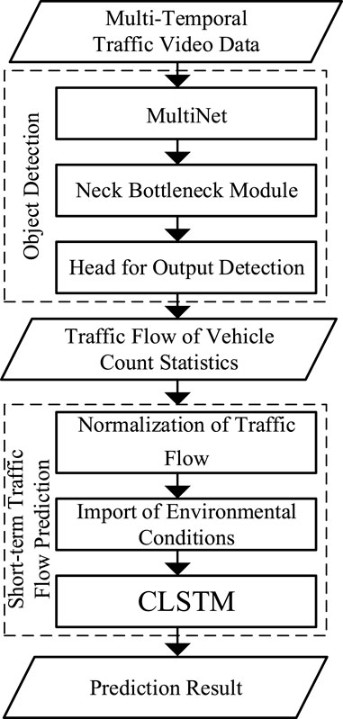
Figure 1 shows the overview of our approach, including two parts. The first part is the vehicle detection and flow extraction from multi-temporal traffic video data, where the core neural network includes the Multi-Net of backbone, neck module for enhancing feature extraction, and head module for detecting the output. In the second part, after normalizing the traffic data, we extracted the feature vector of environmental factors and imported it into an improved LSTM network to predict the traffic flow data under different weather conditions.
2.2 DCN-MultiNet-YOLO
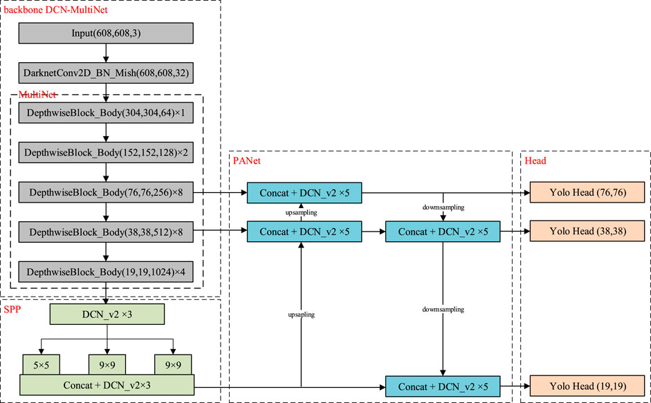
According to the overall structure, target counting methods can be divided into those based on traditional feature extraction (Zhou et al., 2014; Denimal et al., 2017; Li et al., 2020) and those based on the convolutional neural network (CNN) (Yoo et al., 2016; He et al., 2017; Redmon and Farhadi, 2018). Traditional feature extraction methods include the Haar-like feature, the local binary pattern, and histogram of the oriented gradient. The aforementioned algorithm usually focuses on edge feature extraction to detect and count the individual targets, so it requires a high accuracy of edge detection and is not suitable for the counting of overlapping or dense targets. With the development of deep learning, the mainstream object detection and counting algorithms are realized by extracting target object features based on the CNN. On the basis of the original YOLOv3 target detection architecture, YOLOv4 (Bochkovskiy et al., 2020) is optimized in data processing and enhancement (Mosaic), backbone network (Backbone), network training (self-adversarial training), activation function (Mish), and loss function (Focal Loss), which greatly improve the accuracy of target detection and the training efficiency. In the data processing, YOLOv4 obtains the anchor box by clustering the ground-truth box and then uses the Mosaic data enhancement method to label and train targets with different scales. The backbone of YOLOv4 draws on the advantages of extracting deep feature information from deep residual learning [ResNet (He et al., 2016)]. It also adopts the design idea of a spatial pyramid pooling network [Spatial Pyramid Pooling Net (He et al., 2015) Atrous Spatial Pyramid Pooling Net (Liu and Huang, 2019)] to splice arbitrary size feature maps and convert them into fixed output size feature vectors, which can be output at one time to realize multi-scale object detection. The activation function YOLOv4 adopted is mixed with smooth, non-monotonic, and lack of upper bound characteristics. Although its computational complexity is higher than that of ReLu in YOLOv3, its detection effect is improved. In the final loss function training, YOLOv4 uses the idea of focal loss for reference, that is, redistributing the training weights of easy classification samples and difficult classification samples to achieve the accuracy of the two-level detector without losing the network training and prediction speed. Based on the original YOLOv4 network, our approach modifies the framework of backbone and applies the DCN V2 convolution to expand the receptive field of the feature layer and enhance the accuracy of object detection. As shown in Figure 2, the framework of the DCN-MultiNet-YOLO model can be divided into three parts: the backbone of DCN-MultiNet, bottleneck for enhanced feature, and head for detecting output, of which the neck mainly includes the SSP-Net and pyramid attention network. The network parameters of each component are described in detail as follows; the first two units of network parameters in the figure are pixel, and the last is depth. For example, as shown in the figure, the network 608 × 608 × 3 represents an image with a pixel value of 608 × 608 and three channels.
DCN-MultiNet: DCN-MultiNet follows the darknet network in YOLOv4. In order to reduce the parameters of the network structure, multi-convolution layers are used as the core hidden layer of the backbone network. All conventional convolutions in the network framework are replaced by deformable convolutions, which avert possible network accuracy degradation caused by separable convolution. Moreover, we introduced the cross-stage partial network to integrate the gradient changes into the feature map. A smoother Mish is applied instead of the original ReLu as the activation function, which obtains the three types of anchor boxes closest to the real frame by clustering the data in the ground-truth box. Finally, according to the input image with a pixel of 608 × 608×3, the neural network outputs three scale feature maps with shapes of 76 × 76, 38 × 38, and 19 × 19.
Neck: The bottleneck module is designed to enhance the ability of network feature extraction. SSP-Net uses three convolution layers with different shapes to expand the perception threshold of the feature map to the front hidden layer, which can enhance the target recognition ability of the network. SSP-Net also introduces a differentiation pooling strategy, which not only avoids the risk of network overfitting but also outputs fixed size image features. Based on the feature pyramid network (FPN), PANet uses downsampling and upsampling methods to fuse different scale feature maps at the same time so that the output layer after mapping and fusion has richer features and improves the expression ability of the network for shallow feature information and deep semantic information.
Head: The output of the feature map corresponds to the last three feature layers of the backbone network, with shapes of 76 × 76 × 75, 38 × 38 × 75, and 19 × 19 × 75, which has the ability to perform multi-feature layer object detection. The first two dimensions represent the size of the feature map grid, which can extract targets of different shapes. The third dimension is related to the dataset used in network training. If the dataset has 20 categories and the dimensions of location information and category information are five, we should set the layer with a shape of 3 × (20 + 5) to adapt to the anchor box.
To test the detection accuracy of the proposed architecture, we compared the mean average precision between other neural network structures. The formula of precision is as follows:
where P represents the algorithmic precision, TP indicates that a positive sample is correctly retrieved as a positive sample, and a false positive indicates that a negative sample is incorrectly retrieved as a positive sample. The formula for recall is as follows:
where R represents the recall rate of the algorithm, and FN indicates the number of positive samples that were incorrectly retrieved as negative samples. An excellent objection detection model means that the accuracy increases as the recall rate increases. The average precision is obtained by integrating the P–R curves of a class. The formula for the average precision is as follows:
The mean average precision (mAP) is the average of the area under the P–R curve for all categories. The formula for mAP is as follows:
2.3 Conditional Long Short-Term Memory
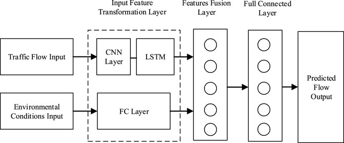
The detected traffic flow from video images, as one of the basic parameters of short-term traffic prediction parameters, can be used as the key basis of traffic decision in the intelligent transportation system (Chen and Chen, 2020). Short-term prediction is to provide short-term (usually 5–10 min) or even real-time traffic prediction based on the traffic data close or exact to the current observation (Petkovics et al., 2015; Fu et al., 2016). Short-term traffic flow prediction is very challenging due to the stochastic and dynamic traffic condition. In recent years, scholars from around the world have conducted widespread and thorough research of LSTM or its variants in short-term traffic flow forecasting with excellent achievements. Ma et al. (2015) developed a long short-term memory (LSTM) neural network to predict the travel speed prediction based on RTMS detection data in Beijing city. The proposed model can capture the long-term temporal dependency for time series and also automatically determine the optimal time window. Zheng et al. (2017) put forward a traffic forecast model based on the LSTM network that considers temporal–spatial correlation in the traffic system via a two-dimensional network composed of many memory units. Du et al. (2020) proposed a deep irregular convolutional residual LSTM network model called DST-ICRL for the urban traffic passenger flow prediction. Little et al. (1981) proposed an end-to-end deep learning architecture that consists of convolution and LSTM to form a Conv-LSTM module to extract the spatial–temporal information from the traffic flow information. Moreover, Ma et al. (2021 and Zheng et al. (Dai et al., 2019; Zheng et al., 2021) proposed an improved LSTM model to improve the accuracy of short-term traffic flow prediction. However, in addition to the traffic flow statistics itself, weather conditions, emergencies, and other external environmental conditions also have great changes on the flow value, which have received less attention in the aforementioned literature studies. The conditional long short-term memory (CLSTM) proposed in this article inputs the aforementioned environmental conditions and traffic flow to the LSTM network and fully connected layer (FC layer), respectively. Then, the output of them is fed into the feature fusion layer (FF layer) and FC layer, which finally export the predicted traffic flow.
Before introducing the structure of the CLSTM, we first described the problem setting of our traffic scenario. The problem of traffic flow prediction can be formulated as follows. First, we divided the total traffic flow into multiple time periods at every
where C means a set containing different environmental conditions.
For example, when we consider
As shown in Figure 3, the proposed CLSTM consists of an input feature transformation layer, a feature fusion layer, and a fully connected layer (FC layer). The traffic flow input is the time series vector
The loss function we selected as the RMSE is the square root of the ratio of the square of the deviation between the value and the actual value, divided by the number of observations. The RMSE used to measure the deviation between the observed value and the actual value is calculated as follows:
Besides the RMSE, we used another two functions—the mean of absolute error (MAE) and mean absolute percentage error (MAPE)—as the accuracy evaluation indicators for comparing these prediction algorithms (Ma et al., 2018; Weng et al., 2018; Xu et al., 2018; Chen C. et al., 2019; Chen F. et al., 2019; Wu et al., 2019) in order to ensure the robustness of the forecast algorithm.
The MAPE represents the average of the absolute values of relative percentage errors, which is calculated as follows:
3 Results and Discussion
3.1 Data and Environment
In this section, we evaluated the performance of the proposed model by using a real-world dataset for object detection and short-term traffic flow prediction. The detailed hardware configuration of this experiment is as follows: the CPU of the computer is Intel (R) core (TM) i9-9900k, the CPU frequency is 3.60 GHz, the memory is 64G, the graphics card model is NVIDIA GeForce RTX 2080ti, and the graphics memory is 11G×2. Our application is deployed on the 64-bit operating system Ubuntu 16.04 with the deep learning frameworks of TensorFlow 1.13.1 and Keras 2.3.1 and the parallel computing framework of CUDA 10. The traffic data were collected at the intersection of Qiaoxiang and Nonglin Roads in Futian District, Shenzhen (Figure 4) between 1 June and 31 July 2021. The weather data come from the China National Meteorological Science Data Center.
3.2 Results for Multi-Target Tracking
The core idea of DCN-MultiNet-YOLO is separable convolution. The standard convolution is decomposed into a depth-wise convolution and a point-wise convolution, which play the role of filtering and linear combination, respectively, in order to reduce the number of parameters and calculation. As mentioned earlier, we used the DCN V2 convolution to expand the receptive domain that can improve the accuracy of the target detection model at the cost of slightly sacrificing the amount of parameters. As can be seen from Table 1, the parameter quantity of DCN-MultiNet-YOLO is only 0.48% more than that of MobileNet and 17% more than that of CSPDarknet. Meanwhile, in order to compare the training time of the algorithm, we set the size of the training batch to 32 and the total training cycle to 200. It is found that when MultiNet is used as the backbone, a single training cycle can cut the training time in half.
In order to verify the detection effect of different algorithms, the second experiment compares the AP results of all categories in the voc2007 + 2012 dataset, which implement the MobileNet and the CSPDarknet53 as backbones in the control group. Figure 5 shows that compared with the YOLOv4 network, whose backbone network is MobileNet and CSPDarknet53, the mAP of DCN-MultiNet-YOLO increased by 13.19% and 6.63%, respectively.

FIGURE 5. AP values of different backbone networks: (A) MobileNet, (B) CSPDarknet, and (C) DCN-MultiNet-YOLO.
In Figure 6, we compared the results of object detection and lane vehicle count of different models. It should be noted that the detection frame rate is related to the currently detected number and training model. The higher the number of detected objects under the same model, the lower is the frame rate. It can be seen from Figure 5 that DCN-MultiNet-YOLO has more current and total detection counts and faster real-time frame rates than that applied to MobileNet and CSPDarknet53 as the backbone in the network.

FIGURE 6. Model test results of different backbone networks: (A) MobileNet, (B) CSPDarknet, and (C) DCN-MultiNet-YOLO.
Finally, we obtained the traffic flow every 5 min in all directions of the Qiaoxiang–Nonglin road using DCN-MultiNet-YOLO. Table 2 shows the example of the obtained traffic flow of six lanes from west to east 7:00 to 9:00 a.m. on 1 June 2021, in which the column numbers represent each 5-min time period during the morning peak hours, and row numbers represent different lanes.
3.3 Results for Short-Term Traffic Flow Prediction
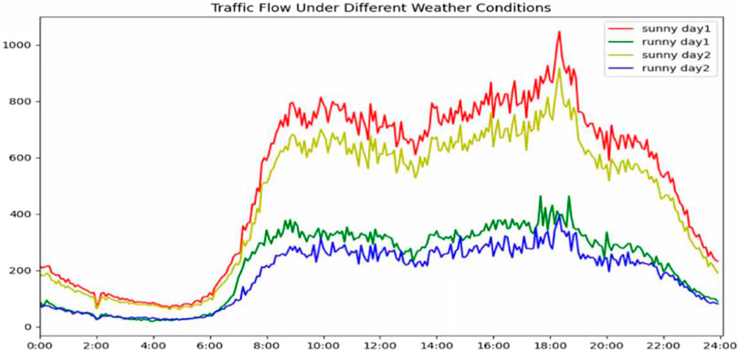
Using the aforementioned object detection algorithm to make traffic statistics on the images of the Qiaoxiang–Nonglin intersection, we can obtain the traffic statistics of the intersection for 2 months. We accumulated the traffic flow of three turns (left, right, and straight) in four directions (east, south, west, and north) every 5 min as a sample. After removing the abnormal data, a total of 5616 sample records were generated by using the traffic flow in 2 months. We used 85% of the aforementioned records as the training set and 15% as the test set. As shown in Figure 7, we first selected 4 days (two sunny days and two rainy days) to analyze the traffic data of the whole day. From the traffic flow data, we can draw the following conclusions: 1) the total traffic flow on rainy days is lower than that on sunny days. This is because the intersection is located in a busy section of Shenzhen, and the rainy days reduce the commuting ability of this road because many vehicles that would have taken this road chose other roads. 2) We compared the correlation coefficient of the two sets of data and found that the correlation coefficient of the two groups of traffic flow data on sunny days is 0.935 and on rainy days it is 0.872, indicating that traffic changes are more random on rainy days, which makes it more difficult to predict.
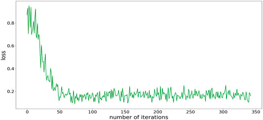
It can be seen from Figure 8 that the loss function of the algorithm decreases with the number of iterations. The loss function begins to converge after about 70 iterations and finally converges to about 0.16. The convergence of the algorithm proves that the traffic prediction method proposed in this article is feasible.
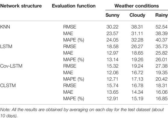
Two kinds of neural network structures—LSTM and Cov-LSTM (Liu et al., 2017)—are compared as benchmarks of the proposed network for prediction performance in this article. We also selected the KNN representative clustering algorithm to compare the accuracy of traffic prediction.
According to Table 3, on the sunny day, the CLSTM has RMSE, MAE, and MAPE values of 15.74, 13.65, and 12.91%, respectively, which are slightly higher than the values of Cov-LSTM of 15.32, 12.06, and 12.71% but lower than those of LSTM and KNN. On non-sunny days (cloudy and rainy days), the proposed module can achieve a smaller prediction error than the other module with all three metrics for all prediction horizons. On the cloudy day, it has RMSE, MAE, and MAPE values of 16.78, 14.34, and 15.19%, respectively, and 18.31, 16.06, and 16.85% on the rainy day. This is because the environmental conditions of the traffic flow are usually interwoven with each other, which can be captured more efficiently by the CLSTM module. The results prove the effectiveness of the proposed model.
Furthermore, we compared the prediction performance of both the benchmark neural network and CLSTM. Although the three network structures can eventually converge and overcome the long-term dependency of RNN, their performances are different. Figure 9 illustrates performance comparison in terms of the predicted traffic volume from 0:00 a.m. to 12:00 p.m. for a 5-min prediction horizon. It can be seen that all three networks have relatively good prediction performance on sunny days. However, the prediction performance of the benchmark network on rainy days is not sufficient. In particular, in the evening and morning rush hours when there is a large fluctuation in traffic volume, the performance advantages of CLSTM are particularly prominent.
4 Conclusion
The grip of traffic flow patterns from multi-temporal images is essential to mitigating urban congestion and can assist in the construction of smart cities. In this article, we made use of 2-month traffic video data for traffic flow monitoring and prediction. We proposed 1) DCN-YOLO, a novel multi-target tracking and counting method for moving targets, which introduced the DCN V2 convolution into the YOLOv4 backbone network and replaced the original CSPDarknet network in order to solve the problem of limited detection accuracy of the MobileNet model. 2) CLSTM, a variant of the LSTM network, which takes the environmental conditions as the feature fusion layers for the short-term traffic flow prediction. Through the case study of one popular road junction in the metropolitan area, the results indicated the better performance of the proposed architecture, of which the mAP of the moving car detection with DCN-YOLO increased by 13.19%, and the prediction RMSE of the CLSTM decreased by 49.01% on rainy days.
Despite the strength of the proposed algorithms in this work, there is still room for improvement. With respect to object detection, it could be necessary to embed depth-wise separable convolution to reduce the number of CSPDarknet53 of the YOLOv4 network to fit for real-time operations at the mobile end. In terms of short-term traffic flow prediction, the current weather conditions can only be described as qualitative variables, such as sunny and rainy days, which limit the prediction accuracy to a certain extent. Future work can include more quantitative factors such as precipitation and air pressure. In addition to factors from the physical environment, human factors, such as driver behaviors under emergency events, can be considered to make the model closer to reality.
Data Availability Statement
The original contributions presented in the study are included in the article/Supplementary Material, further inquiries can be directed to the corresponding author.
Author Contributions
YZ conceived and designed the study and also provided funding; NW contributed to the study design, made improvements to the algorithm, and drafted the manuscript; XL contributed to the data acquisition and experimental study; and LX was involved in data acquisition and revision of the manuscript.
Conflict of Interest
Author NW is employed by Guangzhou Wonping Info-Tech Co., Ltd.
The remaining authors declare that the research was conducted in the absence of any commercial or financial relationships that could be construed as a potential conflict of interest.
Publisher’s Note
All claims expressed in this article are solely those of the authors and do not necessarily represent those of their affiliated organizations, or those of the publisher, the editors, and the reviewers. Any product that may be evaluated in this article, or claim that may be made by its manufacturer, is not guaranteed or endorsed by the publisher.
References
Bochkovskiy, A., Wang, C. Y., and Liao, H. (2020). YOLOv4: Optimal Speed and Accuracy of Object Detection. doi:10.48550/arXiv.2004.10934
Chen, C., Cheng, R., and Ge, H. (2019). An Extended Car-Following Model Considering Driver's Sensory Memory and the Backward Looking Effect. Physica A: Stat. Mech. its Appl. 525, 278–289. doi:10.1016/j.physa.2019.03.099
Chen, F., Song, M., Ma, X., and Zhu, X. (2019). Assess the Impacts of Different Autonomous Trucks' Lateral Control Modes on Asphalt Pavement Performance. Transportation Res. C: Emerging Tech. 103, 17–29. doi:10.1016/j.trc.2019.04.001
Chen, X., and Chen, R. (2020). “A Review on Traffic Prediction Methods for Intelligent Transportation System in Smart Cities,” in 2019 12th International Congress on Image and Signal Processing, BioMedical Engineering and Informatics (CISP-BMEI), Suzhou, China, 19-21 Oct. 2019 (IEEE). doi:10.1109/CISP-BMEI48845.2019.8965742
Dai, G., Ma, C., and Xu, X. (2019). Short-term Traffic Flow Prediction Method for Urban Road Sections Based on Space-Time Analysis and GRU. IEEE Access 7 (99), 143025–143035. doi:10.1109/ACCESS.2019.2941280(
Denimal, E., Marin, A., Guyot, S., Journaux, L., and Molin, P. (2017). Automatic Biological Cell Counting Using a Modified Gradient Hough Transform. Microsc. Microanal 23 (01), 11–21. doi:10.1017/S1431927616012617
Du, B., Peng, H., Wang, S., Bhuiyan, Z. A., Wang, L., Gong, Q., et al. (2020). Deep Irregular Convolutional Residual LSTM for Urban Traffic Passenger Flows Prediction. IEEE Trans. Intell. Transportation Syst. 21 (3), 972–985.
Fu, R., Zhang, Z., and Li, L. (2016). “Using LSTM and GRU Neural Network Methods for Traffic Flow Prediction,” in 2016 31st Youth Academic Annual Conference of Chinese Association of Automation (YAC), Wuhan, China, 11-13 Nov. 2016 (IEEE). doi:10.1109/yac.2016.7804912
He, K., Gkioxari, G., Dollár, P., and Girshick, R. (2017). “Mask R-CNN,” in 2017 IEEE International Conference on Computer Vision (ICCV), Venice, Italy, 22-29 Oct. 2017 (IEEE). doi:10.1109/ICCV.2017.322
He, K., Zhang, X., Ren, S., and Sun, J. (2016). “Deep Residual Learning for Image Recognition,” in 2016 IEEE Conference on Computer Vision and Pattern Recognition (CVPR), Las Vegas, NV, USA, 27-30 June 2016 (IEEE). doi:10.1109/CVPR.2016.90
He, K., Zhang, X., Ren, S., and Sun, J. (2015). Spatial Pyramid Pooling in Deep Convolutional Networks for Visual Recognition. IEEE Trans. Pattern Anal. Machine Intelligence 37 (9), 1904–1916. doi:10.1109/TPAMI.2015.2389824
Khekare, G. S., and Sakhare, A. V. (2013). “A Smart City Framework for Intelligent Traffic System Using VANET,” in 2013 International Mutli-Conference on Automation, Computing, Communication, Control and Compressed Sensing (iMac4s), Kottayam, India, 22-23 March 2013 (IEEE). doi:10.1109/imac4s.2013.6526427
Li, D., Miao, Z., Peng, F., Wang, L., Hao, Y., Wang, Z., et al. (2020). Automatic Counting Methods in Aquaculture: A Review. J. World Aquaculture Soc. 52. doi:10.1111/jwas.12745
Little, J., Kelson, M., and Gartner, N. (1981). MAXBAND: A Program for Setting Signals on Arteries and Triangular Networks. Transportation Res. Rec. J. Transportation Res. Board 795, 40–46.
Liu, S., and Huang, D. (2019). Learning Spatial Fusion for Single-Shot Object Detection. doi:10.48550/arXiv.1911.09516
Liu, Y., Zheng, H., Feng, X., and Chen, Z. (2017). “Short-term Traffic Flow Prediction with Conv-LSTM,” in 2017 9th International Conference on Wireless Communications and Signal Processing (WCSP), Nanjing, China, 11-13 Oct. 2017 (IEEE). doi:10.1109/WCSP.2017.8171119
Ma, C., Dai, G., and Zhou, J. (2021). Short-Term Traffic Flow Prediction for Urban Road Sections Based on Time Series Analysis and LSTM_BILSTM Method. IEEE Trans. Intell. Transport. Syst. (99), 1–10. doi:10.1109/tits.2021.3055258
Ma, C., Hao, W., He, R., and Moghimi, B. (2018). A Multiobjective Route Robust Optimization Model and Algorithm for Hazmat Transportation. Discrete Dyn. Nat. Soc. 2018, 1–12. doi:10.1155/2018/2916391
Ma, X., Tao, Z., Wang, Y., Yu, H., and Wang, Y. (2015). Long Short-Term Memory Neural Network for Traffic Speed Prediction Using Remote Microwave Sensor Data. Transportation Res. Part C: Emerging Tech. 54, 187–197. doi:10.1016/j.trc.2015.03.014
Marais, J., Meurie, C., Attia, D., Ruichek, Y., and Flancquart, A. (2014). Toward Accurate Localization in Guided Transport: Combining GNSS Data and Imaging Information. Transportation Res. Part C: Emerging Tech. 43, 188–197. doi:10.1016/j.trc.2013.11.008
Mckenney, M., and Frey-Spurlock, C. (2018). “Aging in Place: Challenges for Smart & Resilient Communities,” in SIGSPATIAL '18: 26th ACM SIGSPATIAL International Conference on Advances in Geographic Information Systems, November 2018, 1–2. doi:10.1145/3284566.3284567
Petkovics, Á., Simon, V., Gódor, I., and Böröcz, B. (2015). Crowdsensing Solutions in Smart Cities towards a Networked Society. EAI Endorsed Trans. Internet Things 1 (1), e6. doi:10.4108/eai.26-10-2015.150600
Raja, G., Ganapathisubramaniyan, A., Selvakumar, M. S., Ayyarappan, T., and Mahadevan, K. (2018). “Cognitive Intelligent Transportation System for Smart Cities,” in 2018 Tenth International Conference on Advanced Computing (ICoAC), Chennai, India, 13-15 Dec. 2018 (IEEE). doi:10.1109/icoac44903.2018.8939091
Redmon, J., and Farhadi, A. (2018). YOLOv3: An Incremental Improvement. doi:10.48550/arXiv.1804.02767
Tan, Z., and Pan, P. (2019). “Network Fault Prediction Based on CNN-LSTM Hybrid Neural Network,” in 2019 International Conference on Communications, Information System and Computer Engineering (CISCE), Haikou, China, 5-7 July 2019 (IEEE). doi:10.1109/cisce.2019.00113
Telang, S., Chel, A., Nemade, A., and Kaushik, G. (2021). “Intelligent Transport System for a Smart City,” in Security and Privacy Applications for Smart City Development.
Weng, J., Du, G., Li, D., and Yua, Y. (2018). Time-varying Mixed Logit Model for Vehicle Merging Behavior in Work Zone Merging Areas. Accid. Anal. Prev. 117, 328–339. doi:10.1016/j.aap.2018.05.005
Wu, W., Liu, R., Jin, W., and Mac, M. (2019). Stochastic Bus Schedule Coordination Considering Demand Assignment and Rerouting of Passengers. Transportation Res. B: Methodological 121, 275–303.
Xu, X., Šarić, Ž., Zhu, F., and Babić, D. (2018). Accident Severity Levels and Traffic Signs Interactions in State Roads: a Seemingly Unrelated Regression Model in Unbalanced Panel Data Approach. Accid. Anal. Prev. 120, 122–129. doi:10.1016/j.aap.2018.07.037
Yoo, D., Park, S., Lee, J.-Y., Paek, A. S., and Kweon, I. S. (2016). “AttentionNet: Aggregating Weak Directions for Accurate Object Detection,” in 2015 IEEE International Conference on Computer Vision (ICCV), Santiago, Chile, 7-13 Dec. 2015 (IEEE). doi:10.1109/iccv.2015.305
Zear, A., Singh, P. K., and Singh, Y. (2016). Intelligent Transport System: A Progressive Review. Indian J. Sci. Technology 9 (32), 1–8. doi:10.17485/ijst/2016/v9i32/100713
Zhang, L., Zhu, G., Mei, L., Shen, P., Shah, S. A. A., and Bennamoun, M. (2018). “Attention in Convolutional LSTM for Gesture Recognition,” in Proceedings of the 32nd International Conference on Neural Information Processing Systems, 1957–1966.
Zhang, S., Zhao, X., and Tian, Q. (2019). Spontaneous Speech Emotion Recognition Using Multiscale Deep Convolutional LSTM. IEEE Trans. Affective Comput., 1. doi:10.1109/TAFFC.2019.2947464
Zheng, H., Lin, F., Feng, X., and Chen, Y. (2021). A Hybrid Deep Learning Model with Attention-Based Conv-LSTM Networks for Short-Term Traffic Flow Prediction. IEEE Trans. Intell. Transport. Syst. 22 (11), 6910–6920. doi:10.1109/TITS.2020.2997352
Zheng, Y., Guo, R., Ma, D., Zhao, Z., and Li, X. (2020). A Novel Approach to Coordinating Green Wave System with Adaptation Evolutionary Strategy. IEEE Access 8, 214115–214127. doi:10.1109/ACCESS.2020.3037129
Zheng, Z., Chen, W., Wu, X., Chen, P. C. Y., and Liu, J. (2017). LSTM Network: a Deep Learning Approach for Short-Term Traffic Forecast. Iet Intell. Transport Syst. 11 (2), 68–75.
Keywords: multi-target tracking, short-term traffic flow prediction, DCN-MultiNet-YOLO, CLSTM, smart city
Citation: Zheng Y, Li X, Xu L and Wen N (2022) A Deep Learning–Based Approach for Moving Vehicle Counting and Short-Term Traffic Prediction From Video Images. Front. Environ. Sci. 10:905443. doi: 10.3389/fenvs.2022.905443
Received: 27 March 2022; Accepted: 11 April 2022;
Published: 11 May 2022.
Edited by:
Ying Jing, Zhejiang University, ChinaReviewed by:
Wen Xiao, Newcastle University, United KingdomKa Zhang, Nanjing Normal University, China
Copyright © 2022 Zheng, Li, Xu and Wen. This is an open-access article distributed under the terms of the Creative Commons Attribution License (CC BY). The use, distribution or reproduction in other forums is permitted, provided the original author(s) and the copyright owner(s) are credited and that the original publication in this journal is cited, in accordance with accepted academic practice. No use, distribution or reproduction is permitted which does not comply with these terms.
*Correspondence: Nu Wen, d2VubnUxOTg5QDEyNi5jb20=
 Ye Zheng
 Xiaoming Li2