
95% of researchers rate our articles as excellent or good
Learn more about the work of our research integrity team to safeguard the quality of each article we publish.
Find out more
ORIGINAL RESEARCH article
Front. Environ. Sci. , 11 July 2022
Sec. Environmental Informatics and Remote Sensing
Volume 10 - 2022 | https://doi.org/10.3389/fenvs.2022.904939
This article is part of the Research Topic Artificial Intelligence-Based Forecasting and Analytic Techniques for Environment and Economics Management View all 21 articles
 Dashe Li 1,2,3*
 Xuan Zhang 1,2,3*
It is significant to establish a precise dissolved oxygen (DO) model to obtain clear knowledge ablout the prospective changing conditions of the aquatic environment of marine ranches and to ensure the healthy growth of fisheries. However Do in marine ranches is affected by many factors. DO trends have complex nonlinear characteristics. Therefore, the accurate prediction of DO is challenging. On this basis, a two-dimensional data-driven convolutional neural network model (2DD-CNN) is proposed. In order to reduce the influence of missing values on experimental results, a novel sequence score matching-filling (SSMF) algorithm is first presented based on similar historical series matching to provide missing values. This paper extends the DO expression dimension and constructs a method that can convert a DO sequence into two-dimensional images and is also convenient for the 2D convolution kernel to further extract various pieces of information. In addition, a self-attention mechanism is applied to construct a CNN to capture the interdependent features of time series. Finally, DO samples from multiple marine ranches are validated and compared with those predicted by other models. The experimental results show that the proposed model is a suitable and effective method for predicting DO in multiple marine ranches. The MSE MAE, RMSE and MAPE of the 2DD-CNN prediction results are reduced by 51.63, 30.06, 32.53, and 30.75% on average, respectively, compared with those of other models, and the R2 is 2.68% higher on average than those of the other models. It is clear that the proposed 2DD-CNN model achieves a high forecast accuracy and exhibits good generalizability.
DO content of water quality, is necessary for all kinds of aquatic organisms. And changes in DO can reflect changes in the water quality of an aquaculture (Ni et al., 2019). Most fish stop feeding when the oxygen level is lower than 2 mg/L. Large numbers of fish die when the oxygen level is less than 1 mg/L. A low DO content is also a warning sign of eutrophication (Takahashi et al., 2021). To ensure the sound development of fisheries, the accurate prediction and control of DO are necessary tasks in the management of marine ranch fisheries.
Accurate water quality prediction has been challenging due to the complex effects of physical, chemical, biological, hydrometeorological and human-related processes. Some scholars have used traditional machine learning models to predict water quality. Tiyasha et al. (2021) used four types of prediction models, including a random forest (RF), to predict the DO content in the Klang River, Malaysia. Traditional machine learning techniques were applied by Valera et al. (2020) to reconstruct and predict nearshore DO concentrations in small coastal bays. Ahmed and Lin (2021) used a forest of quantile regression models to predict the DO levels in three rivers. Traditional machine learning prediction models can produce effective predictions for small sample sets with relatively simple relationships, but they fail to meet the prediction accuracy requirements for nonlinear, vaguely uncertain water quality features. In light of these problems with traditional machine learning models, the parameter optimization of traditional machine learning models is greatly influenced by human subjective factors. Some models using a meta-learning algorithm for local fine searching and pheromone dynamic updating have emerged. Liu et al. (2014) used an improved particle swarm optimization algorithm and least squares support vector regression to predict the DO content in a crab culture. Heddam and Kisi (2017) proposed an optimally pruned extreme learning machine (OP-ELM), which was newly applied to predict DO concentration with and without water quality variables as predictors. The above literature shows that this hybrid machine learning model can improve the prediction accuracy for DO and overcome the defects of traditional methods. However, its complex modeling methods and steps are still prone to falling into local minima during optimization, so the existing DO prediction models are not intelligent and must still be further improved.
In recent years, many scholars have attempted to predict water quality using neural networks. Compared to traditional predictive models, neural network models have a high self-learning ability and excellent generalizability, allowing them to solve complex nonlinear approximation problems. These methods yield good simulation and prediction effects for trends in the water environment. Zhang et al. (2019) proposed a novel model based on multilayer artificial neural networks (MANNs) and mutual information (MI) to predict the trends of DO. proposed a new clustering-based softplus class-specific extreme learning machine to predict DO changes in time series. Rozario and Devarajan (2021) used a fuzzy C-means clustering method to construct a radial basis function neural network to predict changes in DO. Wu et al. (2018) presented a new model for DO content prediction based on a sliding window, particle swarm optimization, and error backpropagation.
The above models of water quality prediction are based on shallow networks. However, because of the small number of shallow network neurons used, the feature extraction ability of these models is not strong. And the data of some complex functions cannot be used in learning and training. Therefore, some scholars have improved the prediction accuracy of traditional models by developing deep neural network models. Zhi et al. (2021) applied long short-term memory (LSTM) to predict DO levels in several rivers. Cao et al. (2021) proposed a gradient-boosted regression tree algorithm based on an attention gate recurrent unit to predict DO levels in three dimensions. Yaqub et al. (2020) propose a long short-term memory (LSTM)-based neural network and developed to predict the ammonium, total nitrogen, and total phosphorus. Zhu et al. (2021) proposes a DO prediction model incorporating deep learning algorithms of ResNets, BiLSTM, and Attention. The LSTM mentioned above is a recurrent neural structure commonly used in sequence modeling. Compared with the traditional recurrent neural network (RNN), LSTM can alleviate gradient disappearance or explosion problems. However, due to the relatively complex internal structure, the training efficiency is much lower than that of the traditional RNN with the same computational resources, and the training is more difficult overall.
A convolutional neural network (CNN) (Kim, 2017) is a type of feedforward deep neural network containing a convolutional layer, which is composed of five structures: a convolutional layer, a pooling layer, a fully connected layer and a softmax layer. Due to its characteristics of local computation, sparse connection and weight sharing, among the available neural networks, CNNs can effectively reduce network complexity and are robust and fault tolerant. Additionally, CNNs are easy to train and optimize and have been successfully applied in many scientific fields, including computer vision (Hu et al., 2018; Luo et al., 2018), image classification (Sun et al., 2020; Pei et al., 2021), speech recognition (Haque et al., 2020; Song, 2020), natural language processing (Xiao et al., 2020; Yu et al., 2020) and others. Due to the advantages of CNNs in capturing features, they have been increasingly applied in hydrology. Khosravi et al. (2020) used CNN algorithm to develop a flood susceptibility map for Iran.Chen et al. (2020) designed an improved CNN model to establish a CNN calibration approach for the quantitative determination of water pollution with near-infrared data. Barzegar et al. (2020), Barzegar et al. (2021) improved the accuracy of forecasts achieved by a hybrid CNN LSTM deep learning (DL) model. Baek et al. (2020) used a combined CNN-LSTM model for water level and water quality prediction. Yan et al. (2021) predicted water quality using a one-dimensional residual CNN. However, most of the above studies used combined CNN models, which extracted deep features with a CNN and then used another model for prediction. These combined the modeling methods are cumbersome, and they generally adopt a one-dimensional CNN for data feature extraction; however, this approach cannot capture all the relevant spatiotemporal information.
In this paper, an improved 2DD-CNN DO prediction model is proposed. A method for converting a one-dimensional time series into a two-dimensional image is proposed. With this approach, the time dependence of the data is preserved, and the spatial characteristics are obtained. Then, we improve the two-dimensional CNN to perform regression fitting and increase the precision of the prediction model by adding an attention module. The established model strengthens the connections with DO. The main contributions of this article are as follows.
The rest of this article is organized as follows. Section 2 describes the study area and data sources considered in this paper and the proposed study method. Section 3 describes the steps in establishing the 2DD-CNN prediction model. Section 4 analyzes the model prediction performance, compares the 2DD-CNN model with other models and assesses DO data from multiple ranches. Section 5 summarizes the study and the existing modeling problems.
Shandong Province, China, is rich in marine resources, with a coastline length of approximately 2078 kilomiles. The national marine ranch demonstration area accounts for 40% of China, ranking first among the demonstration areas in China. This study included 12 marine ranches along the coastal waters of Shandong Peninsula
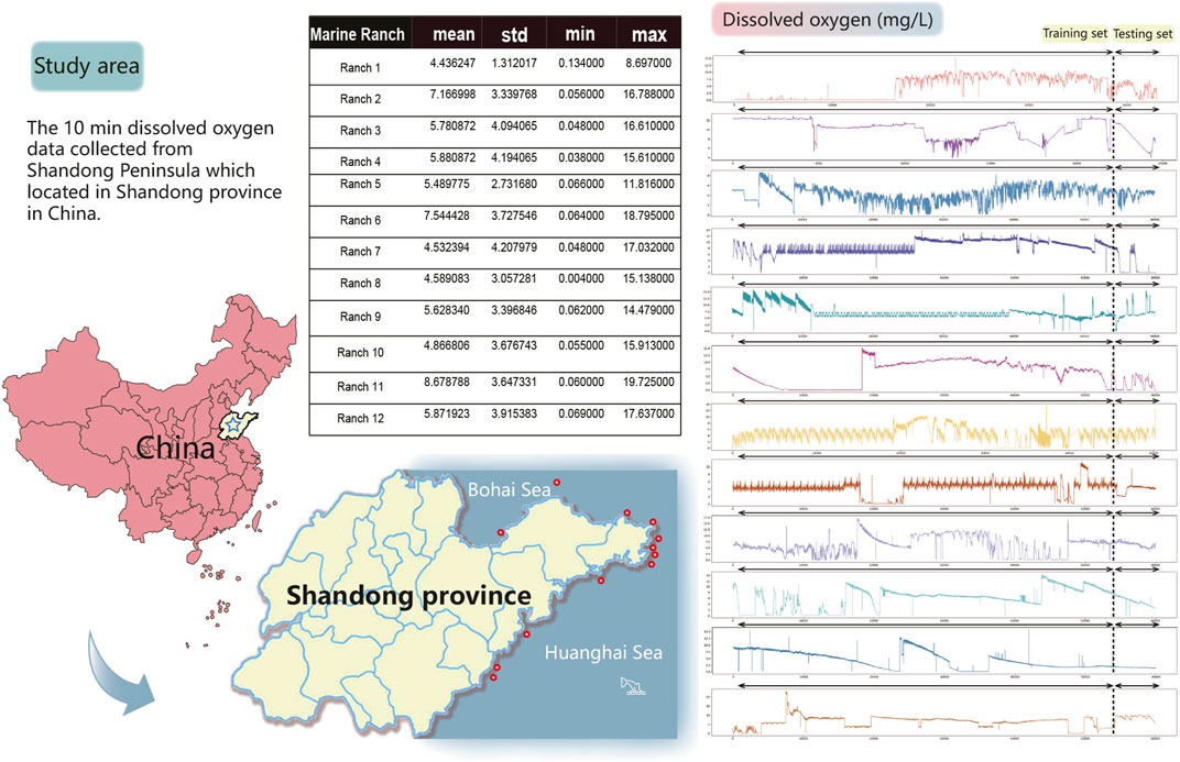
FIGURE 1. Research information of the original data.
In the marine ranch environment, DO data are collected for 10 min, with 144 consecutive samples per day. Notably, 55,000 samples are obtained for each ranch between 2019 and 2021, including 50,000 samples that formed the training set and 5,000 that formed the test set. The same rolling prediction mechanism is used for the training and test sets.
Due to the interference from sensor equipment, the environment and human factors, the collected time series contained some missing values and outliers. Poor-quality datasets containing large numbers of missing values and outliers will result in low-quality forecasting results. Data preprocessing can improve the quality of the data, thus improving the accuracy and performance of the subsequent learning process of the model (Niu and Wang, 2019).
In this paper, we identified the outliers first; then, we removed the outliers and treated them as missing values. Finally, we filled missing values based on the sequence score matching-filling (SSMF) method proposed, as shown in Figure 2. The SSMF approach divides the data into several sets of sequences, determines the score of each set of sequences according to the defined rules, and finds the sequence most similar to the selected sequence based on a score comparison approach, which is regarded as sequence score matching. The next feature in the matching sequence is used to fill the corresponding missing value in the selected sequence. This method is based on featurization. Historical data are used for matching, and the time series trend of historical data is used to estimate the value at the next moment to fill in the data gap. Thus, the problem of discontinuous feature information in training datasets can be avoided.
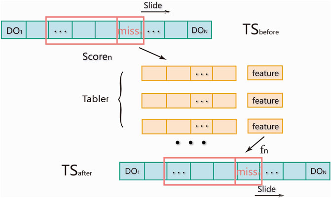
FIGURE 2. SSMF method for filling missing values.
The following symbols are defined for the SSMF process:
• TSbefore = {ts1, ts2, ts3, ⋯tsN−1, tsN}: Original dataset containing missing values, where N is the sequence length;
•
• L: Length of feature sequence;
•
• F [fn−S, fn−S+1, ⋯fn−2, fn−1]: Features dictionary, where f is feature sequence and n ≤ N;
• Tablef [scoren]: The feature query dictionary;
The procedure for filling missing values is as follows.
Step 1: Determine the length of feature sequence. For a time series of length N, the shortest length L of the feature sequence can be obtained according to Eq. 1. To minimize the number of calculations, the number of methods used per L data permutations should be greater than or equal to the total number of time series. Here, L is the length of the feature sequence before the missing values are filled. Let missn be a missing value and n be the missing value’s position in a sequence. In this paper, missing values are postprocessed from L consecutive values.
Step 2: Calculates the probabilities for each category
Step 3: Calculate the feature score of each feature sequence and establish the feature query dictionaryTablef. Consecutive values are regarded as a set of feature sequences denoted as Seq = fn−L, fn−L+1, ⋯fn−2, fn−1, fn. The L+1 value in the feature sequence is regarded as the feature label of the sequence, e.g., F [fn−L, fn−L+1, ⋯fn−2, fn−1, fn] = fn. If the first L features of the feature sequence are known, the corresponding feature scores can be approximated with Eq. 3. All the feature scores for the original sequence are calculated, and the feature dictionary is then established as Tablef [scoren] = fn−L, fn−L+1, ⋯fn−2, fn−1, fn, where
Step 4: A sliding window is used to traverse the original sequence, and the dictionary Tablef is queried to fill the missing values. SSMF fills the missing values in a data sequence. The sliding window is used to traverse the original sequence TSbefore, and the corresponding feature score is calculated according to the L-1 values before the missing value, which are obtained from querying Tablef. Next, the set of features with the closest score is obtained. The consistency among the distribution characteristics of L values and missing values is assessed to find the feature that yields the highest matching score in the feature dictionary. This process is regarded as sequence feature matching, and missn = F [Tablef [scoren]] = fn. This equation returns the processed sequence TSafter.
To realize the transformation of a DO sequence from temporal dependence to spatial dependence, we must reduce the amount of redundant information in the data transformation process. Notably, here, we transform one-dimensional data convertting into two-dimensional images to match the input of the 2DD-CNN, which is used for feature extraction (Ashourloo et al., 2020). In this paper, a method of converting DO data into two-dimensional images is developed, and this approach can effectively learn the characteristics and structures of time series.
The process of constructing a two-dimensional image of DO data in this paper is shown in Figure 3. First, the internal rotation matrix is used to arrange the one-dimensional time series and to transform the one-dimensional time series into a two-dimensional matrix D. D is obtained according to Eq. 4, where k is the number of columns in the matrix.
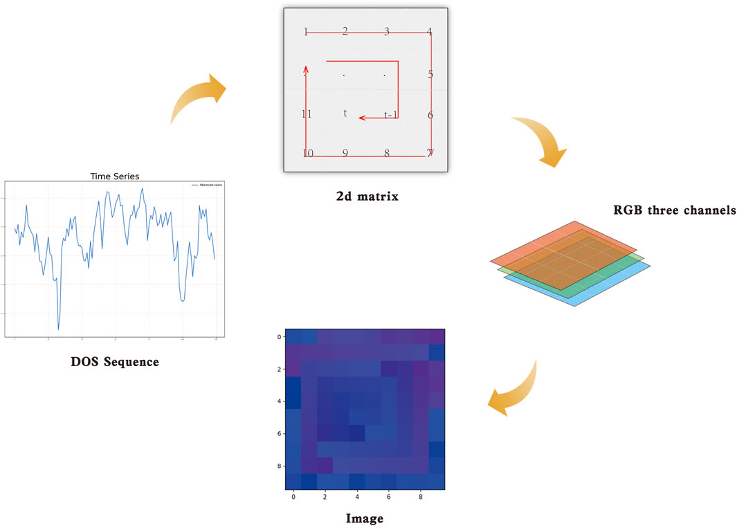
FIGURE 3. Process of constructing two-dimensional image of DO data.
Secondly, the value at each position in the two-dimensional matrix is extended to RGB three-channel form. Specifically, the two-dimensional matrix is transformed into an RGB three-channel image. In the image, each pixel represents a value. According to the color in the image, the overall distribution of pixel values can be intuitively assessed. All values can be uniformly expressed with different colors. The data are stored without loss in three RGB channels. RGB is the color of red, green and blue channels. The R, G, and B channels have 256 levels. Red, green and blue are abbreviated as R,G,B respectively. The brightness of the R, G, and B channels ranges from 0 to 255. Based on these characteristics, this paper divides all the data n into three sets include n1, n2 and n3, n = n1 + n2 + n3, where
The value output by the second channel is Gn:
The value output by the third channel is Bn:
Finally, the PIL image processing library is used, and the resulting image is stored in png lossless format.
The CNN constructed in this paper consists of three parts, namely, a convolutional layer, a pooling layer and a fully connected layer (Jiang et al., 2020; Yang et al., 2021). A linear weighted filter with a local receptive field, namely, a convolution layer, is alternately applied with the pooling layer to sample the extracted features. The fully connected layer distributes the data according to a nonlinear function. The calculation process involving these layers is as follows.
The goals of the convolution layer and pooling layer in the CNN are to extract features and reduce the number of computations. One-dimensional vectors are predicted with the fully connected layer. The overall architecture of the CNN built in this paper is shown in Figure 4. This architecture contains two convolutional layers, two pooling layers and two fully connected layers. The input image is transformed into an input feature matrix. This matrix is then passed through the convolution and pooling layers and then transformed into one-dimensional data before being passed to the fully connected hidden layer and fully connected output layer. Finally, the prediction result is output. In this paper, the CNN architecture shown in Figure 4 is constructed. No upper limit is set for the input window, and the lower limit of the input window is a 4 × 4 matrix.
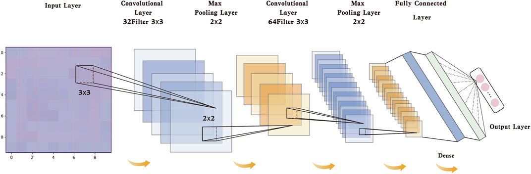
FIGURE 4. Convolutional neural network structure.
The first convolutional layer adopts a 32-layer convolution core of 3 × 3. The second pooling layer adopts a maximum pooling core of 2 × 2. The third convolutional layer uses 64 layers of size 3 × 3. The fourth pooling layer also adopts 2 × 2 maximum pooling. The final layer of the feature graph is flattened to connect the fully connected hidden layer to a one-dimensional vector. The final result is output with the fully connected output layer. The activation function used in the middle layer of the proposed model is a ReLU function. Unlike the traditional classification model, the proposed model does not use an activation function in the final layer, which is used to directly output the final results.
In this paper, a 2DD-CNN is proposed to predict the DO level in marine ranches. The model prediction process is divided into four steps: data preprocessing, constructing the two-dimensional graph of DO data, applying an self-attention module and implementing the 2DD-CNN prediction framework. The process of 2DD-CNN model prediction is shown in Figure 5.
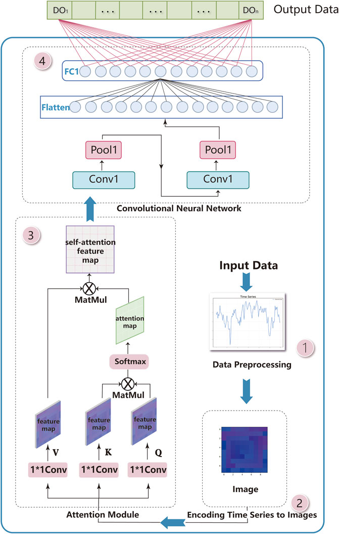
FIGURE 5. Flow chart of DO prediction.
Step 1: Data Preprocessing. The collected DO sequence contains some missing values and outliers. First, the σ principle is used to identify the outliers. This principle can be used to identify low-probability events outside the standard normal distributed interval
Step 2: Encoding Time Series to Images. This step converts a DO sequence into an image. First, the DO sequence is transformed into a two-dimensional matrix by internal rotation. Then, the two-dimensional matrix is mapped to RGB channels. Thus, the transformation of the DO sequence from temporal dependence to spatial dependence is realized.
Step 3: Self-attention Module. To solve the problem, the prediction effect is limited by the local perception of the CNN convolution kernel, the global receptive field is added. In this step, an self-attention mechanism (Wang et al., 2021) is established, and the self-attention module is built before the CNN model (Vaswani et al., 2017; Wang et al., 2018) to mine the influence weight of the information at each position in the matrix based on the available prediction results; then, a new weighting matrix is constructed. The correlation between values is calculated by matrix multiplication. Then, these correlation scores are combined to obtain a weighting matrix. The specific steps are as follows.
Firstly, three 1 × 1 convolution kernels are defined as Wq, Wk, Wv. These kernels are established with the original image to obtain three feature maps, expressed as
Secondly, obtaining the attention map
The partial perception of the CNN convolutional kernels results in each kernel only calculating area information. As the neural network layers deepen, the convolutional kernel region information is limited to only one area. Thus, the regions outside of the convolutional kernel area are not considered, and the effect of prediction is limited. Thus, adding the self-attention module to the model is a good way to solve this problem.
Step 4: 2DD-CNN Prediction Network Framework. First, the number and order of convolutional and pooling layers are determined, and the detailed structure is shown in Figure 4. Second, the ratio of training data to verification data is set as 16:1, and the trained back-propagation 2DD-CNN is used. The initial values of the weight and bias parameters in the input layer and output layer of 2DD-CNN are set. Then, the input dataset size and output dataset size are determined according to the 2DD-CNN features. Finally, the model is optimized by the root mean square prop (RMSProp) algorithm. Based on repeated experimental analyses, the prediction effect based on the 2DD-CNN is the best when the model parameters are learningrate = 0.02, batchsize = 15 and epochs = 100. The trained model is used in the prediction of DO levels.
To verify the model proposed in this paper, the 2DD-CNN is used to predict the oxygen sequences for 12 ranches. A comparison experiment with other algorithms and a generalization experiment involving multiple ranches are performed. The Python 3.8 language is used in the experiments, and the hardware included an Inter(R)Core(TM) i5-8265 CPU at3.30 GHz and 8 GB memory.
To verify the excellent performance of the 2DD-CNN model and analyze the errors between the predicted and observed values of the model, this paper applies five measurement indices: the mean square error (MSE), mean absolute error (MAE), root mean square error (RMSE), mean absolute percentage error (MAPE) and coefficient of determination (R2). The corresponding mathematical expressions are given in Equations 12–14, Equation 15 and Equation 16, where
In this case, 55,000 DO values from the Luhaifeng marine ranch in Qingdao are used as an example, Data from other Marine ranches were analyzed in the same way as the focus of the study. The data are divided into a training set and test set at a 10:1 ratio. Under the same conditions, the 2DD-CNN is compared with other models. The comparison model includes a CNN, an LSTM model, CNN-LSTM, a back Propagation Neuron Network (BP) (Zhang and Lou, 2021), a decision tree (DT) (Anmala and Turuganti, 2021), a RF (Karijadi and Chou, 2022), dynamic evolving neural fuzzy inference system (DENFIS) (Adnan et al., 2019), a group method of data handling (GMDH) neural networks (Adnan et al., 2020) a hybrid model based on long short-term memory neural network and ant lion optimizer (LSTM-ALO) (Yuan et al., 2018), a hybrid model based on an optimally pruned extreme learning machine (OP-ELM) and a hybrid model based on the least squares support vector machine and gravitational search algorithm (LSSVM–GSA) (Zeng et al., 2021).
Figure 6 shows the prediction results based on 600 observations from the test set and various prediction models. The 2DD-CNN model and other models exhibit good performance in predicting trends. For comparison, we enlarge part of the plot of 71 data points showing the 2DD-CNN predictions. Notably, among all the predictions, these values are closest to the observed values. Specifically, the lag of the neural network prediction model is obvious. The prediction effects of the LSTM model and the LSTM’s hybrid model are second to that of the 2DD-CNN. The results in Figure 6 show that the prediction effect of the 2DD-CNN is generally superior to that of the other models.
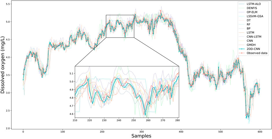
FIGURE 6. The DO content prediction results.
The experimental results of all models are further verified by comparing the corresponding evaluation indics MSE, MAE, RMSE, MAPE, and R2. The results are shown in Table 1. The predicted values of the 2DD-CNN display the lowest MSE, MAE, MAPE and RMSE and the highest R2, corresponding to the lowest prediction error. Compared with LSTM, the 2DD-CNN reduces the MSE, MAE, RMSE and MAPE of the predictions by 45.8, 26.21, 26.4 and 26.3%, respectively. Compared with BP, the 2DD-CNN reduces the MSE, MAE, RMSE and MAPE of the predictions by 13.8, 18.3, 7.2 and 18.95%, respectively. Compared with RF, the 2DD-CNN reduces the MSE, MAE, RMSE and MAPE of the predictions by 87.7, 57.6, 58.4 and 58.8%, respectively. Compared with DT, the 2DD-CNN reduces the MSE, MAE, RMSE and MAPE of the predictions by 79.0, 53.13, 54.19 and 54.56%, respectively. Compared with DENFIS, the 2DD-CNN reduces the MSE, MAE, RMSE and MAPE of the predictions by 54.94, 24.8, 32.87 and 25.34%, respectively. Compared with GMDH, the 2DD-CNN reduces the MSE, MAE, RMSE and MAPE of the predictions by 82.00, 56.22, 57.58 and 57.24%, respectively. Compared with the traditional CNN prediction model, the 2DD-CNN reduces the MSE, MAE, RMSE and MAPE of the predictions by 51.49, 31.06, 30.35 and 29.9%, respectively. Compared with CNN-LSTM, the 2DD-CNN reduces the MSE, MAE, RMSE and MAPE of the predictions by 73.33, 52.52, 48.35 and 49.42%, respectively. Compared with LSTM-ALO, the 2DD-CNN reduces the MSE, MAE, RMSE and MAPE of the predictions by 59.04, 20.52, 36.00 and 23.77%, respectively. Compared with OP-ELM, the 2DD-CNN reduces the MSE, MAE, RMSE and MAPE of the predictions by 59.20, 20.59, 31.13 and 23.92%, respectively. Compared with LSSVM-GSA, the 2DD-CNN reduces the MSE, MAE, RMSE and MAPE of the predictions by 49.37, 27.31, 28.84 and 1.63%, respectively. On average, the MSE of predictions obtained with the 2DD-CNN is 51.63% lower than that obtained with other models, the MAE is 30.06% lower, the RMSE is 32.53% lower, the MAPE is 30.75% lower and the R2 is 2.68% higher. From the comparison of the results, the 2DD-CNN model performs significantly better than the other models in predicting DO levels. Additionally, the existing CNN prediction models performed worse than the studied LSTM and BP models. Nevertheless, the prediction performance of the improved 2DD-CNN model is better than that of all of the other models. In summary, improving the CNN to establish the 2DD-CNN model proposed in this paper yields a significant improvement in the accuracy of DO prediction.
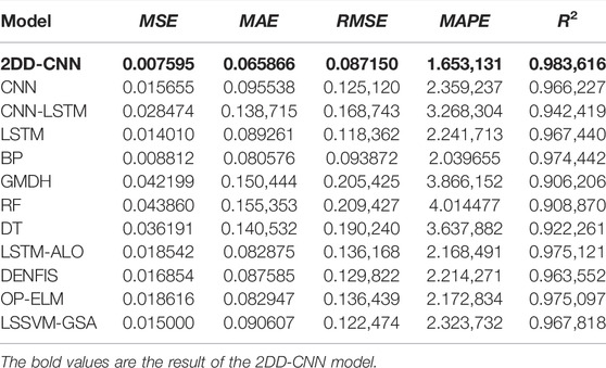
TABLE 1. Comparison of evaluation indexes of model prediction error.
Figure 7 shows a box plot of the predicted and observed DO values for eleven models in individual marine ranches. The 2DD-CNN predictions are similar to the observed values overall. The other model results differ from the observed values based on the upper quartile, mean, maximum and minimum values. The upper limits of the predicted values of the LSTM model and DT model are similar to the upper limit of the observed values. However, the values obtained with the 2DD-CNN are most similar to the observed values based on the mean value, upper and lower quartiles and lower limit. The BP model, RF model and DENFIS model results largely differed from the observed values based on the upper and lower quartiles and the upper and lower limits. The range of predicted values of the BP model is smaller than the range of observed values, with predictions concentrated near the mean value; this result indicates that the prediction of maximum and minimum values by the BP model is not accurate. The prediction range of the RF model exceeds that of the observed values, and the prediction of extreme values is inaccurate. The prediction range of RF model exceeds the observed values, and the prediction of extreme values is also inaccurate. The DENPFIS model is not very accurate in predicting the results at lower values. Compared with the observed values, the values predicted by the CNN model and CNN-LSTM model moved upward overall. The data of the predicted values and observed value of the hybrid model had great similarities on the whole, but some outliers appeared in the model prediction, which might have been due to model overfitting. In conclusion, the prediction accuracy of the BP model, RF model and DT model is not good. Other CNN models, the CNN-LSTM model and the LSTM-ALO model have certain deviations in prediction, and the models must be adjusted. The DENFIS, GMDH, OP-ELM, and LSSVM-GSA models have poor prediction effects on some outliers and edge values. The data distributions of the 2DD-CNN-predicted values and observed values are very close.
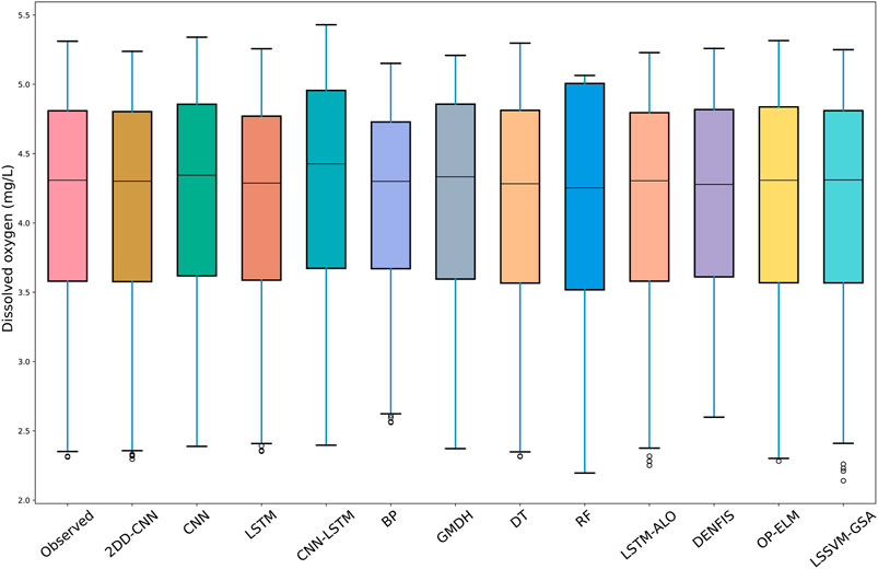
FIGURE 7. Comparison of predicted and observed values of DO for different models.
Figure 8 shows the Taylor diagram of the performance of ten models. The scattered dots in the figure represent the model, the radiating lines represent the correlation coefficients, the horizontal and vertical axes represent the standard deviations, and the semicircular dotted lines represent the RMSE. Figure 8A shows the whole part of the Taylor diagram, and 8 B shows the enlarged display of eleven model indicators. For the prediction of DO, the discrete correlation coefficient, standard deviation and RMSE proposed in this paper are 0.991,817, 0.988,898 and 0.1280, respectively, and the prediction result is the best. Based on the observed values, the closer that a value is to the red dot representing the observed value in the Taylor diagram, the better that the prediction performance is. In summary, the prediction of DO proposed in this paper is the best.
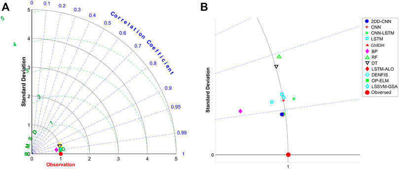
FIGURE 8. Comparison of predicted and observed values of DO for different models. (A) is a whole Taylor diagram, and (B) is a partially enlarged Taylor diagram.
To further analyze the prediction ability of the models, the prediction results for 144 samples each day with different models are presented in the form of line charts and density correlation graphs. Figure 9 shows the values predicted by each model compared to the observed values. In Figure 9, the data predicted by the model proposed in this paper are closest to the observed values, and the prediction effect of peaks and valleys is the best among all models. We analyze the correlation between the predicted and observed values based on the density correlation plot in Figure 9. In this figure, the closer that a scatter point is to the light-colored dotted line, the closer that the predicted values is to the corresponding observed value. The line fit based on the scatter point is the dark dotted line.
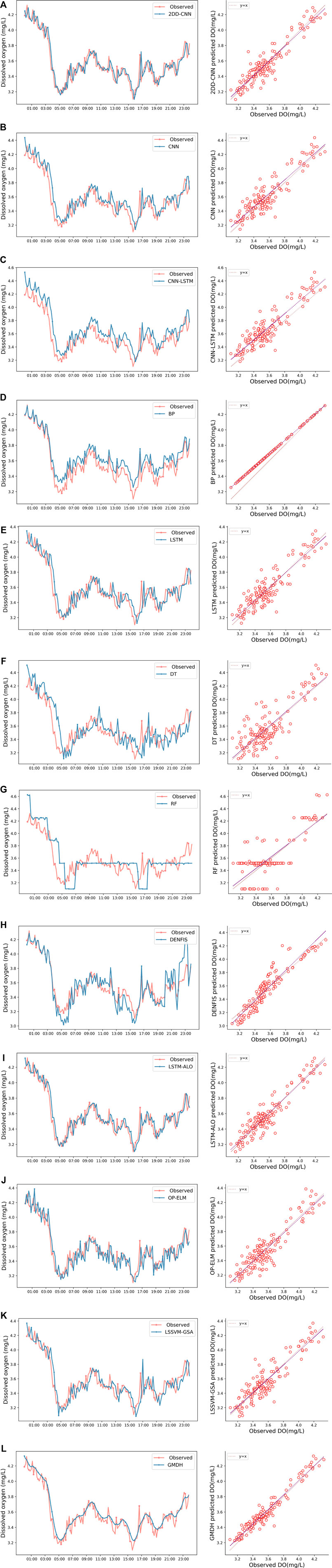
FIGURE 9. Comparison of predicted and observed values of DO for multiple models. (A) is the result of 2DD-CNN. (B) is the result of CNN. (C) is the result of CNN-LSTM. (D) is the result of BP. (E) is the result of LSTM. (F) is the result of DT. (G) is the result of RF. (H) is the result of DENFIS. (I) is the result of LSTM-ALO. (J) is the result of OP-ELM. (K) is the result of LSSVM-GSA. (L) is the result of GMDH.
This outcome can be clearly observed in the figure. The graph in Figure 9A shows that the predicted values of 2DD-CNN is almost the same as the observed DO, indicating good performance. The graph on the right of Figure 9A shows that all points are located near the straight line, and the linear regression line of these points almost covers the straight line. This outcome shows that 2DD-CNN can predict DO data with high accuracy. Figure 9B shows the prediction results of the CNN. Compared with the curves in Figures 9A,B, the predicted values of the CNN are more difference from the observed values than are predicted values of 2DD-CNN. Compared with the right figure of Figures 9A,B, the fitted line is farther from the y = x line, and the point dispersion is greater. This outcome indicates that the prediction effect of the CNN model is inferior to that of 2DD-CNN. The model in this paper is an improvement on the CNN model. Compared with the CNN model, the self-attention module is added to the model in this paper, and two-dimensional convolution is adopted. The results show that the improved model improves the prediction accuracy of DO. In the line chart in Figure 9C, the values predicted by the CNN and CNN-LSTM models exhibit obvious variations in positions compared with the positions of the observed values. These differences are clear in the density correlation diagram in Figure 9D, which shows the predicted value of the BP model. As a shallow neural network, the BP has the characteristics of a simple structure. However, due to limited neurons and shallow networks, the accuracy is not as good as the predicted value of the deep neural network in the fitting experiment of complex DO trends. In Figure 9E, the prediction accuracy of the LSTM model and LSTM’s hybrid are second only to that of the 2DD-CNN. As an RNN model, LSTM can meet most accuracy requirements, but the training efficiency is not high due to its relatively complex internal structure. There is some deviation between the predicted and observed values in the line chart and density correlation diagram. The values predicted by the BP, DT and RF models in Figure 9F, Figure 9G and Figure 9H, respectively, deviate from the observed values, and the prediction of peaks and valleys is not accurate. Additionally, the RF can only predict the general trend of the DO. Two traditional machine learning models, DT and RF, perform poorly in fitting complex nonlinear DO data. Figure 9H shows the predicted value of the DENFIS model. DENFIS performs poorly in predicting the peak value, showing a situation of amplifying the peak value and underestimating the value. In the density correlation diagram, it can also be observed that the predicted values of the DENFIS model deviate greatly from the observed values compared with the medium-high value segment and the low-value segment. As a mathematical fuzzy inference model, DENFIS is not as effective as a deep learning model in predicting DO. Figures 9I,J,K show the prediction effects of the LSTM-ALO, OP-ELM and LSSVM-GSA models, respectively, in comparison with the hybrid model. The parameters of the deep learning LSTM model, shallow ELM neural network, GMDH and LSSVM-GSA machine learning model were optimized using a metaheuristic algorithm. The prediction results showed good performance with slight errors. Although the model parameters were optimized to a large extent, the structure of the model remained unchanged. The prediction accuracy is still limited by the model itself, which is not as accurate as the model proposed in this paper. The operation process of the hybrid model is complicated. The above experimental analysis indicates that 2DD-CNN not only outperforms the other models in predicting DO but also performs better in predicting peaks and valleys, displaying the best overall fit to observations.
DO data from 12 marine ranches are used as samples to verify and evaluate whether 2DD-CNN could be applied to analyze DO data from different marine ranches with large environmental differences. In this paper, the DO level is predicted for 12 h in 12 ranches in the research area. The lowest value reached approximately 0.2 mg/L, and the highest value reached approximately 15 mg/L. All the data selected in this paper are sufficiently representative.
The predicted results are shown in Figure 10, and comparisons of predicted and observed values for each ranch are shown through line charts and density correlation plots. The 2DD-CNN displays good performance for all the considered ranches, and the blue predictions and red observations exhibit high overlap. The positive correlation reaches a maximum when the value is 1 in the density correlation diagram. Generally, when r exceeds 0.5, a strong correlation exists. The correlation between the predicted and observed values is more than 0.7 for all ranches with the 2DD-CNN model.
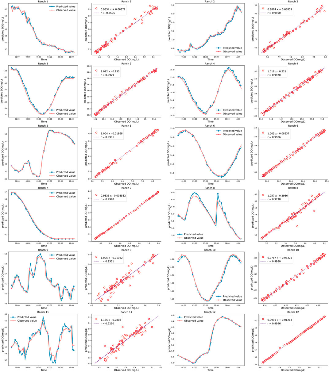
FIGURE 10. Application of the model to data from different ranches.
The correlation between the predicted and observed values for ranches 2, 3, 4, 5, 6, 7, 10 and 12 reached greater than 0.99. The fitting lines of the scatter plots in the density correlation map are very close to y = x, with a small inclination and small intercept. The line chart and density correlation diagram for each ranch show that 2DD-CNN exhibits good performance in predicting peak and valley values, and the agreement between the fitting line and points in the density correlation diagram is high. The model best predicts the DO values for ranches 3, 4, 6, 7, 10 and 12, but the results are not as good for ranches 1, 2, 8, 9 and 11. Notably, the DO data for ranches 3, 4, 6, 7, 10, and 12 are relatively smooth, but in other cases, the data contain a small amount of noise. Although the predicted DO in cases with noise is not as good as that in other cases, the prediction results still display high accuracy; thus, even if DO data contain a small amount of noise, the model can still achieve accurate predictions.
The MSE, MAE, MAPE, RMSE and R2 are used to measure the accuracy of the 2DD-CNN in DO prediction for multiple marine ranches, as shown in Table 2 and Figure 11. The MSE, MAE, MAPE, RMSE for all ranches are very low, and R2 is greater than 0.97. Figure 11 illustrates a three-part radar diagram. Figure 11A shows the MSE of the predicted and observed values for 12 ranches. The MSEs vary for different ranches but are all below 0.02. Figure 11B shows the MAE of the predicted and observed values for 12 ranches. In Figure 11B, the MAEs of multiple ranches displayed in the radar chart are similar to those in Figure 11A, with values below 0.08. Figure 11D shows the RMSE of the predicted and observed values for 12 ranches with values below 0.2. Figure 11E shows the MAPE of the predicted and observed values for 12 ranches with values below 2. Figure 11C shows the R2 results based on the predicted and observed values for the 12 ranches. In Figure 11C, an almost circular shape is observed because all values are close to 1. In summary, by analyzing and evaluating the predicted DO values for 12 marine ranches, we find that the 2DD-CNN can effectively forecast DO data in different intervals and in cases with different influencing factors. Thus, the model displays strong generalization ability.
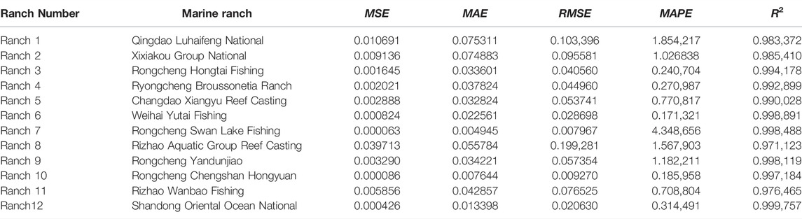
TABLE 2. Prediction error evaluation indexes of 12 ranch models.
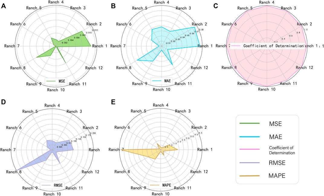
FIGURE 11. Radar diagrams of the prediction error evaluation indexes for 12 ranches based on the model proposed in this paper. (A) is the value of MSE. (B) is the value of MAE. (C) is the value of RMSE. (D) is the value of MAPE. (E) is the value of R2.
In this part, we will discuss the research results of 2DD-cnn from the aspects of missing value filling, time series transformation into image work and convolution neural network prediction model, so as to further discuss the effectiveness and progressiveness of the proposed dissolved oxygen prediction method. Each section is discussed below.
Common data filling methods generally include providing KNN(Qi et al., 2021) data, interpolation, means, medians, etc., and returning the predicted values for the model. The former algorithm is simple, and the characteristics represented by the filled-in data are too singular. Although the predicted value of the latter filling model can accurately match the changes in the time series, the modeling process of the algorithm is too complex. In this paper, we propose a new SSMF algorithm to provide the missing values. This method uses the sequence before the missing value to match the historical data, defines the historical sequence feature as the score formula, considers the historical feature sequence as the decision reference object of the missing value, and takes the final entries of the most similar historical data as the missing value, thereby rendering the provided data more reliable. Usually, we observe the sequence according to whether there are similar fragments in past periods of time. The correlation between the past time series and the current time series and the subsequences related to the past will be used for decision-making regarding the current time point. Similar to this method, the logic is also the method of providing the predicted value of the model, such as using a machine learning model like RF (Deng et al., 2019) to pretest and provide the value after learning the historical data, but the method proposed in this paper is simpler and does not require modeling. Our algorithm can capture the sequence features, and the amount of computation is only O(n). The accuracy of the provided data is guaranteed, while the calculation is simple.
In order to obtain more accurate prediction, we should use as many features embedded in time series as possible in the prediction model. Recent studies have shown that by converting one-dimensional time series data into two-dimensional images in some way, more features embedded in the original time series can be retained. Therefore, a new framework is explored to visualize time series, so as to learn the features and structures of time series with the help of the success of deep learning in the field of computer vision. However, at present, most of the research on time series focuses on the classification of time series. For example, A time series classification method based on CNN and recursive graph is proposed (Hatami et al., 2018). In this method, firstly, the recursive graph is used to convert the time series into two-dimensional texture images. Yang et al. (2019) proposed a framework for sensor classification using multivariate time series sensor data as input, which encodes multivariate time series data into two-dimensional color images. However, we propose a novel framework for encoding time series as two-dimensional images to predict DO, this method preserves the time series information in the form of matrix arrangement. At the same time, in addition to the adjacent data, the periodic data or interval data also contain some rules and characteristics. We think that the closer the data is, the more meaningful it is. Therefore, this cyclotron arrangement method transforms the time information into spatial information to a certain extent. The method of transforming sequences into two-dimensional pictures proposed in this paper aims to mine various forms of information, and is also convenient for two-dimensional convolution kernel to further extract a variety of information. We use the method of converting dissolved oxygen data into two-dimensional pictures and inputting them into convolutional neural network, which rarely appears in the study of dissolved oxygen prediction. Moreover, according to the experiment in Section 4.2, the prediction accuracy of our proposed method is higher than that of other models.
The long-term dependence of the capture sequence plays an important role in deep learning prediction models. However, the convolution operation has a significant weakness in that it only operates on a local neighbourhood, thus missing global information (Bello et al., 2019). With the deepening of the network, there has always been the problem of local calculation, limiting the performance of the model. To resolve this problem, this paper uses a self-attention mechanism to improve the CNN. The self-attention mechanism is a variant of the attention mechanism, decreasing the dependence on external information. A self-attention mechanism is used to mine the influence weight of information at each position in the input matrix on the prediction results, which can accurately capture the internal correlation of data or features and better assist the optimization process of CNN models (Jia et al., 2021). Its application in DO sequence prediction is mainly through calculating the interaction between DO sequences, to solve the problem of long-distance dependence. The self-attention mechanism is a variant of the attention mechanism, decreasing the dependence on external information, and it is better at capturing the internal correlation of data or features. At this time, the CNN prediction model is more focused on capturing the characteristics of the input matrix. Through the learning of feedforward neural networks, we can better consider the context information of time series.
Because the aquatic environment of marine pastures is affected by various factors, the change in DO is complex and nonlinear. To improve the prediction accuracy for DO, the change trend in it can be accurately predicted. In this paper, an improved 2DD-CNN DO prediction model is proposed. In the pretreatment stage, an SSMF method is proposed to provide missing values, and a new method is used to convert the time series of water quality parameters into pictures and input them into a two-dimensional CNN. At the same time, the two-dimensional CNN model is improved, and a convolutional self-attention module is added to the network to resolve the long-distance dependence problem by calculating the interaction between DO sequences. The model proposed in this paper achieves good improvement in prediction accuracy. The 2DD-CNN model has a very good prediction effect and exhibits good generalizability for the prediction error, fitting degree, peak valley value and data segments with large and gentle fluctuations. This model is applicable not only to the prediction of one water quality parameter but also to the prediction of other water qualities. The prediction of water quality parameters plays an important role in marine ranch management by providing quantitative information for the solution of emerging environmental problems and the decision-making of sustainable management.
Although 2DD-CNN has achieved good results in predicting DO, there remain many aspects that can be improved. First, DO data preprocessing has a significant impact on the accuracy of data modeling and is an important method to improve the accuracy of DO prediction. In the method that the SSMF used to provide missing values in this paper, parameter optimization is greatly affected by human subjective factors and cannot ensure the optimization of set parameters. Therefore, optimizing SSMF parameters will be the focus of the next improvement. Second, the research in this paper only involves the prediction of one-dimensional DO, but due to the interaction of water quality parameters of marine pastures, DO is affected by many water quality parameters. To further capture the variation characteristics of DO, predicting DO according to multidimensional water quality parameters is an important research direction. In addition, the method of transforming time into images designed in this paper could store more feature data, so further research work could be performed in the direction of feature expression in the future to better mine the internal relationships of data and to improve the prediction accuracy.
The original contributions presented in the study are included in the article/Supplementary Material, further inquiries can be directed to the corresponding authors.
DL designed the study and revised the manuscript. XZ performed the study and wrote the manuscript. DL and XZ revised the manuscript. All authors approved the publication of the final manuscript.
This work is supported in part by the National Natural Science Foundation of China under Grants 61772319, 61472227, and 61602277; the Yantai Science and Technology Innovation Development Project (2022YTJC06003022).
The authors declare that the research was conducted in the absence of any commercial or financial relationships that could be construed as a potential conflict of interest.
All claims expressed in this article are solely those of the authors and do not necessarily represent those of their affiliated organizations, or those of the publisher, the editors and the reviewers. Any product that may be evaluated in this article, or claim that may be made by its manufacturer, is not guaranteed or endorsed by the publisher.
The Supplementary Material for this article can be found online at: https://www.frontiersin.org/articles/10.3389/fenvs.2022.904939/full#supplementary-material
Adnan, R. M., Liang, Z., El-Shafie, A., Zounemat-Kermani, M., and Kisi, O. (2019). Prediction of Suspended Sediment Load Using Data-Driven Models. Water 11, 2060. doi:10.3390/w11102060
Adnan, R. M., Liang, Z., Parmar, K. S., Soni, K., and Kisi, O. (2020). Modeling Monthly Streamflow in Mountainous Basin by Mars, Gmdh-Nn and Denfis Using Hydroclimatic Data. Neural Comput. Applic. 33, 2853–2871. doi:10.1007/s00521-020-05164-3
Ahmed, M. H., and Lin, L.-S. (2021). Dissolved Oxygen Concentration Predictions for Running Waters with Different Land Use Land Cover Using a Quantile Regression Forest Machine Learning Technique. J. Hydrol. 597, 126213. doi:10.1016/j.jhydrol.2021.126213
Anmala, J., and Turuganti, V. (2021). Comparison of the Performance of Decision Tree (DT) Algorithms and Extreme Learning Machine (ELM) Model in the Prediction of Water Quality of the Upper Green River Watershed. Water Environ. Res. 93, 2360–2373. doi:10.1002/wer.1642
Ashourloo, D., Shahrabi, H. S., Azadbakht, M., Rad, A. M., Aghighi, H., and Radiom, S. (2020). A Novel Method for Automatic Potato Mapping Using Time Series of Sentinel-2 Images. Comput. Electron Agric. 175, 105583. doi:10.1016/j.compag.2020.105583
Baek, S.-S., Pyo, J., and Chun, J. A. (2020). Prediction of Water Level and Water Quality Using a Cnn-Lstm Combined Deep Learning Approach. Water 12, 3399. doi:10.3390/w12123399
Barzegar, R., Aalami, M. T., and Adamowski, J. (2020). Short-term Water Quality Variable Prediction Using a Hybrid CNN-LSTM Deep Learning Model. Stoch. Environ. Res. Risk Assess. 34, 415–433. doi:10.1007/s00477-020-01776-2
Barzegar, R., Aalami, M. T., and Adamowski, J. (2021). Coupling a Hybrid Cnn-Lstm Deep Learning Model with a Boundary Corrected Maximal Overlap Discrete Wavelet Transform for Multiscale Lake Water Level Forecasting. J. Hydrol. 598, 126196. doi:10.1016/j.jhydrol.2021.126196
Bello, I., Zoph, B., Vaswani, A., Shlens, J., and Le, Q. V. (2019). “Attention Augmented Convolutional Networks,” in Proceedings of the IEEE/CVF International Conference on Computer Vision (ICCV), October 27 – November 2, 2019, Seoul, 3286–3295. doi:10.1109/iccv.2019.00338
Cao, X., Ren, N., Tian, G., Fan, Y., and Duan, Q. (2021). A Three-Dimensional Prediction Method of Dissolved Oxygen in Pond Culture Based on Attention-Gru-Gbrt. Comput. Electron. Agric. 181, 105955. doi:10.1016/j.compag.2020.105955
Chen, H., Chen, A., Xu, L., Xie, H., Qiao, H., Lin, Q., et al. (2020). A Deep Learning Cnn Architecture Applied in Smart Near-Infrared Analysis of Water Pollution for Agricultural Irrigation Resources. Agric. Water Manag. 240, 106303. doi:10.1016/j.agwat.2020.106303
Deng, W., Guo, Y., Liu, J., Li, Y., Liu, D., and Zhu, L. (2019). A Missing Power Data Filling Method Based on Improved Random Forest Algorithm. Chin. J. Electr. Eng. 5, 33–39. doi:10.23919/CJEE.2019.000025
Haque, M. A., Verma, A., Alex, J. S. R., and Venkatesan, N. (2020). “Experimental Evaluation of Cnn Architecture for Speech Recognition,” in First International Conference on Sustainable Technologies for Computational Intelligence, August 22–26, 2020, Shenzhen (Springer), 507–514. doi:10.1007/978-981-15-0029-9_40
Hatami, N., Gavet, Y., and Debayle, J. (2018). “Classification of Time-Series Images Using Deep Convolutional Neural Networks,” in Tenth International Conference on Machine Vision (ICMV 2017), November 13–15, 2017, Vienna, Austria (International Society for Optics and Photonics), 106960Y. doi:10.1117/12.2309486
Heddam, S., and Kisi, O. (2017). Extreme Learning Machines: a New Approach for Modeling Dissolved Oxygen (Do) Concentration with and without Water Quality Variables as Predictors. Environ. Sci. Pollut. Res. 24, 16702–16724. doi:10.1007/s11356-017-9283-z
Hu, J., Shen, L., and Sun, G. (2018). “Squeeze-and-excitation Networks,” in Proceedings of the IEEE Conference on Computer Vision and Pattern Recognition, June 18–22, 2018, Salt Lake City, USA, 7132–7141. doi:10.1109/cvpr.2018.00745
Jia, M., Gao, Y., Li, S., Yue, J., and Ye, M. (2021). An Explicit Self-Attention-Based Multimodality Cnn In-Loop Filter for Versatile Video Coding. Multimed. Tools Appl., 1–15. doi:10.1007/s11042-021-11214-2
Jiang, H., Zhang, C., Qiao, Y., Zhang, Z., Zhang, W., and Song, C. (2020). Cnn Feature Based Graph Convolutional Network for Weed and Crop Recognition in Smart Farming. Comput. Electron. Agric. 174, 105450. doi:10.1016/j.compag.2020.105450
Karijadi, I., and Chou, S.-Y. (2022). A Hybrid Rf-Lstm Based on Ceemdan for Improving the Accuracy of Building Energy Consumption Prediction. Energy Build. 259, 111908. doi:10.1016/j.enbuild.2022.111908
Khosravi, K., Panahi, M., Golkarian, A., Keesstra, S. D., Saco, P. M., Bui, D. T., et al. (2020). Convolutional Neural Network Approach for Spatial Prediction of Flood Hazard at National Scale of iran. J. Hydrol. 591, 125552. doi:10.1016/j.jhydrol.2020.125552
Kim, P. (2017). “Convolutional Neural Network,” in MATLAB Deep Learning (California and La Jolla, CA: Springer), 121–147. doi:10.1007/978-1-4842-2845-6_6
Liu, S., Xu, L., Jiang, Y., Li, D., Chen, Y., and Li, Z. (2014). A Hybrid WA-CPSO-LSSVR Model for Dissolved Oxygen Content Prediction in Crab Culture. Eng. Appl. Artif. Intell. 29, 114–124. doi:10.1016/j.engappai.2013.09.019
Luo, H., Xiong, C., Fang, W., Love, P. E. D., Zhang, B., and Ouyang, X. (2018). Convolutional Neural Networks: Computer Vision-Based Workforce Activity Assessment in Construction. Automation Constr. 94, 282–289. doi:10.1016/j.autcon.2018.06.007
Ni, W., Li, M., Ross, A. C., and Najjar, R. G. (2019). Large Projected Decline in Dissolved Oxygen in a Eutrophic Estuary Due to Climate Change. J. Geophys. Res. Oceans 124, 8271–8289. doi:10.1029/2019JC015274
Niu, X., and Wang, J. (2019). A Combined Model Based on Data Preprocessing Strategy and Multi-Objective Optimization Algorithm for Short-Term Wind Speed Forecasting. Appl. Energy 241, 519–539. doi:10.1016/j.apenergy.2019.03.097
Pei, Y., Huang, Y., Zou, Q., Zhang, X., and Wang, S. (2021). Effects of Image Degradation and Degradation Removal to Cnn-Based Image Classification. IEEE Trans. Pattern Anal. Mach. Intell. 43, 1239–1253. doi:10.1109/tpami.2019.2950923
Qi, X., Guo, H., and Wang, W. (2021). A Reliable Knn Filling Approach for Incomplete Interval-Valued Data. Eng. Appl. Artif. Intell. 100, 104175. doi:10.1016/j.engappai.2021.104175
Rozario, A. P. R., and Devarajan, N. (2021). Monitoring the Quality of Water in Shrimp Ponds and Forecasting of Dissolved Oxygen Using Fuzzy C Means Clustering Based Radial Basis Function Neural Networks. J. Ambient. Intell. Hum. Comput. 12, 4855–4862. doi:10.1007/s12652-020-01900-8
Song, Z. (2020). English Speech Recognition Based on Deep Learning with Multiple Features. Computing 102, 663–682. doi:10.1007/s00607-019-00753-0
Sun, Y., Xue, B., Zhang, M., Yen, G. G., and Lv, J. (2020). Automatically Designing Cnn Architectures Using the Genetic Algorithm for Image Classification. IEEE Trans. Cybern. 50, 3840–3854. doi:10.1109/TCYB.2020.2983860
Takahashi, S., Hori, R. S., Yamakita, S., Aita, Y., Takemura, A., Ikehara, M., et al. (2021). Progressive Development of Ocean Anoxia in the End-Permian Pelagic Panthalassa. Glob. Planet. Change 207, 103650. doi:10.1016/j.gloplacha.2021.103650
Tiyasha, T., Tung, T. M., Bhagat, S. K., Tan, M. L., Jawad, A. H., Mohtar, W. H. M. W., et al. (2021). Functionalization of Remote Sensing and On-Site Data for Simulating Surface Water Dissolved Oxygen: Development of Hybrid Tree-Based Artificial Intelligence Models. Mar. Pollut. Bull. 170, 112639. doi:10.1016/j.marpolbul.2021.112639
Valera, M., Walter, R. K., Bailey, B. A., and Castillo, J. E. (2020). Machine Learning Based Predictions of Dissolved Oxygen in a Small Coastal Embayment. J. Mar. Sci. Eng. 8, 1007. doi:10.3390/jmse8121007
Vaswani, A., Shazeer, N., Parmar, N., Uszkoreit, J., Jones, L., Gomez, A. N., et al. (2017). “Attention Is All You Need,” in Advances in Neural Information Processing Systems, California and La Jolla, CA: Neural Information Processing Systems, 5998–6008.
Wang, X., Girshick, R., Gupta, A., and He, K. (2018). “Non-local Neural Networks,” in Proceedings of the IEEE Conference on Computer Vision and Pattern Recognition, June 18–22, 2018, Salt Lake City, USA, 7794–7803. doi:10.1109/cvpr.2018.00813
Wang, Y., Zhang, Z., Feng, L., Ma, Y., and Du, Q. (2021). A New Attention-Based Cnn Approach for Crop Mapping Using Time Series Sentinel-2 Images. Comput. Electron. Agric. 184, 106090. doi:10.1016/j.compag.2021.106090
Wu, J., Li, Z., Zhu, L., Li, G., Niu, B., and Peng, F. (2018). Optimized Bp Neural Network for Dissolved Oxygen Prediction. IFAC-PapersOnLine 51, 596–601. doi:10.1016/j.ifacol.2018.08.132
Xiao, X., Zhang, D., Hu, G., Jiang, Y., and Xia, S. (2020). CNN-MHSA: A Convolutional Neural Network and Multi-Head Self-Attention Combined Approach for Detecting Phishing Websites. Neural Netw. 125, 303–312. doi:10.1016/j.neunet.2020.02.013
Yan, J., Liu, J., Yu, Y., and Xu, H. (2021). Water Quality Prediction in the Luan River Based on 1-drcnn and Bigru Hybrid Neural Network Model. Water 13, 1273. doi:10.3390/w13091273
Yang, C.-L., Chen, Z.-X., and Yang, C.-Y. (2019). Sensor Classification Using Convolutional Neural Network by Encoding Multivariate Time Series as Two-Dimensional Colored Images. Sensors 20, 168. doi:10.3390/s20010168
Yang, X., Zheng, C., Zou, C., Gan, H., Li, S., Huang, S., et al. (2021). A Cnn-Based Posture Change Detection for Lactating Sow in Untrimmed Depth Videos. Comput. Electron. Agric. 185, 106139. doi:10.1016/j.compag.2021.106139
Yaqub, M., Asif, H., Kim, S., and Lee, W. (2020). Modeling of a Full-Scale Sewage Treatment Plant to Predict the Nutrient Removal Efficiency Using a Long Short-Term Memory (Lstm) Neural Network. J. Water Process Eng. 37, 101388. doi:10.1016/j.jwpe.2020.101388
Yu, S., Liu, D., Zhu, W., Zhang, Y., and Zhao, S. (2020). Attention-based Lstm, Gru and Cnn for Short Text Classification. J. Intell. Fuzzy Syst. 39, 333–340. doi:10.3233/JIFS-191171
Yuan, X., Chen, C., Lei, X., Yuan, Y., and Muhammad Adnan, R. (2018). Monthly Runoff Forecasting Based on Lstm-Alo Model. Stoch. Environ. Res. Risk Assess. 32, 2199–2212. doi:10.1007/s00477-018-1560-y
Zeng, F., Nait Amar, M., Mohammed, A. S., Motahari, M. R., and Hasanipanah, M. (2021). Improving the Performance of LSSVM Model in Predicting the Safety Factor for Circular Failure Slope through Optimization Algorithms. Eng. Comput, 1–12. doi:10.1007/s00366-021-01374-y
Zhang, D., and Lou, S. (2021). The Application Research of Neural Network and BP Algorithm in Stock Price Pattern Classification and Prediction. Future Gener. Comput. Syst. 115, 872–879. doi:10.1016/j.future.2020.10.009
Zhang, Y., Fitch, P., Vilas, M. P., and Thorburn, P. J. (2019). Applying Multi-Layer Artificial Neural Network and Mutual Information to the Prediction of Trends in Dissolved Oxygen. Front. Environ. Sci. 7, 46. doi:10.3389/fenvs.2019.00046
Zhi, W., Feng, D., Tsai, W.-P., Sterle, G., Harpold, A., Shen, C., et al. (2021). From Hydrometeorology to River Water Quality: Can a Deep Learning Model Predict Dissolved Oxygen at the Continental Scale? Environ. Sci. Technol. 55, 2357–2368. doi:10.1021/acs.est.0c06783
Keywords: convolutional neural network, self-attention mechanism, dissolved oxygen, marine ranch, prediction
Citation: Li D and Zhang X (2022) Utilizing a Two-Dimensional Data-Driven Convolutional Neural Network for Long-Term Prediction of Dissolved Oxygen Content. Front. Environ. Sci. 10:904939. doi: 10.3389/fenvs.2022.904939
Received: 26 March 2022; Accepted: 17 June 2022;
Published: 11 July 2022.
Edited by:
Yiliao Song, University of Technology Sydney, AustraliaReviewed by:
Salim Heddam, University of Skikda, AlgeriaCopyright © 2022 Li and Zhang . This is an open-access article distributed under the terms of the Creative Commons Attribution License (CC BY). The use, distribution or reproduction in other forums is permitted, provided the original author(s) and the copyright owner(s) are credited and that the original publication in this journal is cited, in accordance with accepted academic practice. No use, distribution or reproduction is permitted which does not comply with these terms.
*Correspondence: Dashe Li , MjAxNTEzMTAxQHNkdGJ1LmVkdS5jbg==; Xuan Zhang , MjAyMDQxMDAxMEBzZHRidS5lZHUuY24=
Disclaimer: All claims expressed in this article are solely those of the authors and do not necessarily represent those of their affiliated organizations, or those of the publisher, the editors and the reviewers. Any product that may be evaluated in this article or claim that may be made by its manufacturer is not guaranteed or endorsed by the publisher.
Research integrity at Frontiers
Learn more about the work of our research integrity team to safeguard the quality of each article we publish.