Climate change impact assessment on a tropical river resilience using the Streeter-Phelps dissolved oxygen model

This paper provides a technical analysis of a river’s current and future resilience in a watershed with intensive agricultural and fishing activities. The study area was the last section of the Culiacan River corresponding to the river mouth over a lagoon system. Dissolved oxygen modeling was performed using the Streeter-Phelps model to evaluate the river self-depuration capability using Biochemical Oxygen Demand, dissolved oxygen, streamflow, and water temperature data from 2013 to 2020. Fieldwork was carried out to establish the geomorphological characteristics of the river by determining stream velocity, width, and depth and the location of nine sources of pollution on the river. The modeling was performed for three groups of months with different temperatures, identified by hierarchical cluster analysis. Estimates were made for future scenarios, assessing the effect of climate change on the Culiacan River’s self-depuration capability. The results showed that most of the year, the degradation rate of the system results in rapid assimilation of organic matter. However, the modeling indicates that the river would lose its resilience capability under climate change. Thus, it is essential to implement wastewater treatment systems to reduce the environmental impact on the aquatic ecosystem in the river and the lagoon system.

1 Introduction

Climate change refers to a change in the state of the climate recorded at a local, regional, or global level that can be identified by the variability of its properties (IPCC 2019). Over the long term, this variability has caused alterations in the environmental characteristics such as ocean acidification, melting glaciers, depletion of water reserves, pressure over terrestrial and marine systems (which are food producers), and higher diffusion of persistent organic pollutants (León-Cortés et al., 2018; He et al., 2018). Climate change has been associated with either global conditions of warming or cooling. The negative impact on the water quality of water bodies is related to the temperature increase. The most studied impacts are the solubility decrease of the dissolved oxygen (DO) and changes in the nitrification and eutrophication processes (Rodríguez 2020).

The wastewater discharges cause a decrease in the DO concentration in the receiving aquatic bodies. The accelerated population growth has contributed to the DO reduction, and nowadays, it has caused the loss of environmental services in surface water bodies (e.g., rivers and dams) (Tehreem et al., 2020). Furthermore, the increasing temperature and the reduction of the ecological flow increase the severe consequences for ecosystems, such as modifying the conditions in habitats, decreasing the species yield, and damaging ecological processes and the ecosystem’s features (Häder and Barnes 2019). It was estimated that the planet’s temperature will increase by 1.5°C between 2030 and 2052 (IPCC 2019). In addition, in 2100, the warming can be between 3 and 4°C above the current average temperature (IPCC 2019).

Climate change affects the temperature of the surface water bodies. A research group evaluated the effect of the environmental conditions and morphometric parameters on the temperature change of 10 lakes in Poland (Czernecki and Ptak, 2018). That analysis is based on the historical measurements (1971–2015), which showed a trend in which the average annual temperature increases by 0.37°C in the lake’s surface water. The future changes in the surface temperature in the lakes were based on simulations of 33 Atmosphere-Ocean General Circulation Models (AOGCMs) available in the project Coupled Model Intercomparison Project 5 (CMIP5) for Representative Concentration Pathway (RCP): 2.6, 4.5, 6.0, and 8.5. The scenes indicated an increase in the lake’s water temperature from 1.4°C (RCP 2,6) to 4.2°C (RCP 8.5) from 2081 to 2100. The developed empirical-statistical scale reduction models use the air temperature field as the predictor. The scenes indicated an increase in the lake’s water temperature from 1.4°C (RCP 2,6) to 4.2°C (RCP 8.5) for 2081–2100.

Yang et al. (2019) identified a causal relationship between climate change and anthropogenic activities on the increase of temperature of eleven lakes. The study was performed through a cluster analysis, with the K-means method, in three types of lakes: natural, semi-urban, and urban lakes. The results show a warming trend from 2001 to 2017, according to the annual average lake surface water temperature (day/night) and the near-surface air temperature in the eleven lakes. For the lake surface water temperature, urban lakes warming is more evident than the warming in semi-urban and natural lakes, which signals the significant impact of human activities on the lake surface water temperature.

Changes in land use cause direct and indirect impacts on water bodies, inducing alterations in the water quality. For example, the nutrient loads are increased from agricultural and domestic wastewaters (Mendivil-García et al., 2020; Paudel and Cargo 2021). Mainly, intensive agriculture produces higher water stress in basins due to 65%–85% of its freshwater requirement.

Sinaloa is the most important agricultural state in Mexico. In 2020, 10,675.26 km² of land was cultivated, where 11, 803, 854 t of food was produced, implying more than $3,055 billion (CODESIN 2021). Culiacan River (CR) supplies water for the irrigation of 2,734.75 km² of cropland, with a value of $885,860 (CODESIN 2019), and supplies water for 2,316,427 inhabitants (INEGI 2021). Furthermore, the basin of CR flows out in the Gulf of California, over the lagoon system of Altata-Ensenada del Pabellon. The agricultural drainage of the CR area provides 37,132 t/yr of inorganic nitrogen and 1,695 t/yr of inorganic phosphorous, which contributes to the decrease in the salinity of the bay in which the River flows out (Mendivil-García et al., 2020). Consequently, poor water quality in the River would have disastrous effects on the coastal ecosystems and fish production.

There are three critical influencing factors on the CR’s future water quality: Agricultural land use, agricultural wastewater with high agrochemical content, and climate change effect. These factors compromise the environmental services, such as food production (fishing and agriculture). A numerical model application with accurate measurements and temperature trends could help quantify the effect of those three key factors in CR.

The aquatic ecosystems can resist anthropogenic activities and the climate change effect; this capability is resilience (Fuller et al., 2019). In order to evaluate the resilience of a water body, mathematical models have been developed considering the main mechanisms of pollutants transport, aeration, and natural microbial purification (Quiroz-Fernández et al., 2018). Among the most advanced models, QUAL2E, WASP, WASP-IPX, SWRRBWQ, and MIKE 11 are fourth-generation models (Bui et al., 2019; Kamal et al., 2020). However, the high degree of complexity in the structure and dynamics of the aquatic ecosystems and the natural stochastic character have halted the formulation of a complete, general, and dynamic model suitable for developed countries.

The Streeter-Phelps model is broadly used for water quality modeling under DO balance in water bodies. This model considers the DO consumption by aerobic microorganisms responsible for organic matter oxidation and the input of DO by the reaeration process. This recovery in the DO levels depends on the hydraulic characteristics of rivers (Mendes et al., 2020). The Streeter-Phelps model has been used successfully in diverse latitudes to evaluate the resilience of surface water bodies in front of agricultural, domestic, and industrial discharges (Arifin et al., 2019; Wahyuningsih et al., 2020).

Studies have been conducted to relate climate change and water bodies’ resilience. Generalized methods of moments have been implemented to assess the impact of average temperature, energy demand, and population growth on water stress. The results show that the water quality is affected by the high energy demand and the industrialization process; it was found that rapid industrialization and low water quality are the liable factors for infant mortality in the region studied (Tehreem et al., 2020).

Three models of terrestrial area (LPJmL-DGVM, INLAND-DGVM, and ORCHIDEE) were used to analyze the impact of deforestation and climate change in terms of the hydrology in the Amazon Basin. In addition, three General Circulation Models were used to correct the climate in the three scenarios generated. The results estimate that the temperature in the Amazonic region will increase by 3.3°C, producing a decrease of 31% in the minimum discharge of the River at the end of this century (Guimberteau et al., 2017).

Projections resulting from climate change, nutrient loads, and the phytoplankton production in freshwater were performed employing the following two climatic simulations: the hydrologic model Soil and Water Assessment Tool (SWAT) and the ecologic model AQUATOX (Pesce et al., 2018). The results show an increase of 5°C for 2100, with the base period with a RCP of 4.5. With a RCP of 8.5, an increase of 7°C was projected. Moreover, the nitrogen and phosphorous trends increment from 50 to 300% in the winter period and variations in the phytoplankton species.

Nowadays, a few studies have been carried out to evaluate the resilience of water bodies considering climate change by employing mathematical models. The existing studies focus on evaluating of the water availability rather than the water quality. There are no models that objectively quantify the combined effect of agriculture, wastewater discharge, and climate change on the surface water quality in Mexico. Models are necessary to determine the future water features and, under these scenarios, to propose preventive actions for the conservation and suitable distribution of water in Mexico.

This work aims to generate and analyze future scenarios about the water quality in a representative tropical river (mainly in developing countries), using kinetic and hydrologic basis considering the variability under climate change trends. Moreover, the resilience of the River is evaluated with mathematical models so that the decision-makers use this technical information to formulate development plans.

2 Methods

The prediction of water quality of tropical rivers involved the use of a dynamic model (not static) and quantify factors such as hydrological, kinetic (chemical and biochemical), and climatological. This parameterization of variables also requires the incorporation of the dynamic aspect within the model itself. In the present study, hydrological, hydraulic, kinetic, and water quality methodologies, as well as a calibrated deterministic modeling, and their coupling to climate change trends were followed in sequence. In each stage, information was obtained experimentally for the greatest possible certainty of the results. Figure 1 shows the steps of the overall methodology. Subsequently, Sections 2.1–2.8 describe the steps in detail that were carried out to achieve the research objective.

FIGURE 1

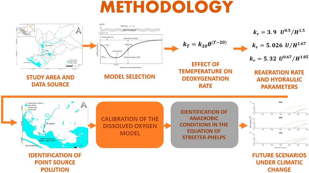
FIGURE 1. Flowchart Methodology.

2.1 Study area and data source

CR is the mainstream of the Culiacan Basin with a warm semi-arid climate and Mexico’s highest agricultural and fishing activities. It is the second biggest basin in the country in terms of drained area, which achieves 19,150 km². In the coastal region of the basin, the main economic activities are fishing and agriculture. Fishing activities produce 353,604 t of food, with a commercial value of $556,393 (SIAP 2020).

The selected transect used for parameterization of the model (Section 2.2) was located between the geographical coordinates (24.6284, −107.661) and (24.4936, −107.7323). In this section, the National Water Commission in Mexico (CONAGUA) installed three monitoring points: the site RH10-2 Sinaloa (24.6284, −107.661), Culiacan River 1 (24.4976, −107.732), and the point Culiacan River 2 (24.5319, −107.71) (Figure 2), where water quality data such as DO, BOD, COD and Temperature are recorded bimonthly. These points correspond to 6 km upstream of the river mouth. The CR mouth is located on the lagoon system of Altata-Ensenada de Pabellón. In this system are six fishing villages, where fishing engages 74% of the population. The lagoon system Altata-Ensenada del Pabellon is the habitat of bivalve mollusks, shrimps, scales fishes, sharks and rays (INAPESCA 2019). Furthermore, this system is one of Mexico’s central natural wetland systems (DOF 2019).

FIGURE 2

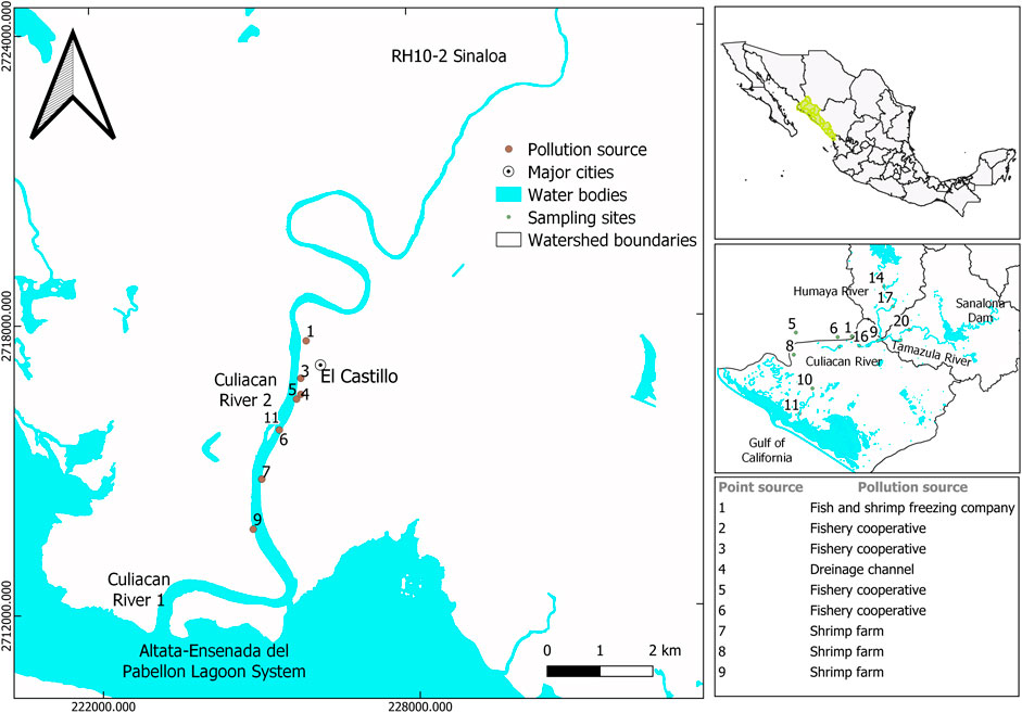
FIGURE 2. The transect of study on the Basin of the Culiacan River for the DO modeling.

2.2 Model selection and parameterization

Streeter-Phelps model was selected because it requires a minimum of historical data and represents the water body behavior under the effect of a point source pollution (Long 2020). The point and diffuse sources of pollution in the Culiacan Basin hinder the application of the water quality model the fourth generation. Despite the simplicity of the Streeter-Phelps model, its accuracy increases as the kinetic and hydraulic variables are measured in situ and laboratory (de Victorica-Almeida 2003). Moreover, this model is easy to use and converges quickly, unlike fourth generation models. Eq. 1 is the Streeter-Phelps model used for the DO simulation in this work.

$\mathit{D}=\frac{{\mathit{k}}_{\mathit{d}}{\mathit{L}}_{\mathbf{0}}}{{\mathit{k}}_{\mathit{r}}{\mathit{k}}_{\mathit{d}}}\left({\mathit{e}}^{-{\mathit{k}}_{\mathit{d}}\mathit{t}}-{\mathit{e}}^{-{\mathit{k}}_{\mathit{r}}\mathit{t}}\right)+{\mathit{D}}_{\mathbf{0}}{\mathit{e}}^{-{\mathit{k}}_{\mathit{r}}\mathit{t}}(1)$

Where D is the dissolved oxygen deficit (saturation DO—DO) (mg/L); L₀ is the ultimate BOD of the mixture of stream water and wastewater (mg/L); k_d is deoxygenation rate, 1/d, k_r is reaeration rate, 1/d; t is the elapsed time between discharge point and distance downstream; D₀ is the initial oxygen deficit of the mixture of river and wastewater (mg/L).

The critical point equals the deficit´s critical time (tc), which shows the lowest point on the DO sag curve profile. At this point, stream conditions are at their worst. Setting the derivative of the oxygen deficit equal to zero and solving for the critical time yields on Eq. 2.

${\mathit{t}}_{\mathit{c}}=\frac{\mathbf{1}}{{\mathit{k}}_{\mathit{r}}-{\mathit{k}}_{\mathit{d}}}\mathit{ln}\left\{\frac{{\mathit{k}}_{\mathit{r}}}{{\mathit{k}}_{\mathit{d}}}\left[\mathbf{1}-\frac{{\mathit{D}}_{\mathbf{0}\left({\mathit{k}}_{\mathit{r}}-{\mathit{k}}_{\mathit{d}}\right)}}{{\mathit{k}}_{\mathit{d}}{\mathit{L}}_{\mathbf{0}}}\right]\right\}(2)$

2.3 Effect of temperature on deoxygenation rate

The deoxygenation rate (k_d) is the rate of contaminants biodegradation by aerobic heterotrophic microorganisms (Benedini and Tsakiris 2013).

Annual and monthly averages of temperature were determined from 2013 to 2020 (Supplementary Appendix S1, Supplementary Table S1). Temperature data was processed by cluster analysis using the Linkage method (Nearest Neighbor), a dissociative method. The data were grouped according to internal homogeneity and external heterogeneity (Tanuk et al., 2019). This way, groups of months with similar water temperatures were determined, and a kd was calculated for each group using the Arrhenius equation (Eq. 3). The microbial activity, and kd, are directly proportional to temperature. It is possible to determine the relationship between the reaction rate constant and the temperature with the Arrhenius equation.

${\mathit{k}}_{\mathit{d}}={\mathit{k}}_{\mathbf{20}}{\mathit{\theta }}^{(\mathit{T}-\mathbf{20})}(3)$

Where k₂₀ = rate reaction under a standard reference of 20°C in laboratory conditions, and θ = Arrhenius constant, 1.047.

2.4 Reaeration rate and hydraulic parameters

For the determination of reaeration (kr) were used the O′ Conner-Dobbins Model (Eq. 4), the Churchill (Eq. 5), and Owens-Gibbs methods (Eq. 6). These equations consider the same parameters: kr is oxygen replenishment at the interface between the stream and the atmosphere; U is stream velocity (m/s), and H is the stream’s depth (m).

${\mathit{k}}_{\mathit{r}}=\mathbf{3.9}\mathit{ }{\mathit{U}}^{\mathbf{0.5}}/{\mathit{H}}^{\mathbf{1.5}}(4)$

${\mathit{k}}_{\mathit{r}}=\mathbf{5.026}\mathit{ U}/{\mathit{H}}^{\mathbf{1.67}}(5)$

${\mathit{k}}_{\mathit{r}}=\mathbf{5.32}\mathit{ }{\mathit{U}}^{\mathbf{0.67}}/{\mathit{H}}^{\mathbf{1.85}}(6)$

Depth measurement was performed in the sites RH10-2, Culiacan River 2, and Culiacan River 1; an echo sounder ECHOTEST II—Plastimo was used. The river’s speed was measured with a flow meter LOVI (USGS 2010) according to the protocols. The average speed of the current and average depth was 0.289 m/s and 2.5–3 m, respectively. The hydraulic and morphological characteristics match the applicability interval of the O'Connor-Dobbins equation, which considers columns with depths between 0.30 and 9.14 m, and a flow velocity from 0.15 to 0.49 m/s (Table 1).

TABLE 1

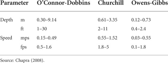
TABLE 1. Ranges of depth and velocity to develop the O’Connor-Dobbins, Churchill, and Owens-Gibbs formulas for stream reaeration.

2.5 Identification of the point sources of pollution

The studied section identified nine discharges of the coastal area as point sources (Figure 1). These discharges correspond to the effluents released from a seafood freezer, four fishing cooperatives, a shrimp farm with a production of 306 t, and a drainage channel (Table 2). All these effluents discharge into the Culiacan River and are situated along 6 km (Figure 1). When applying the Streeter-Phelps model, only the point source of site 9 was considered because this site considers the cumulative effects of all previous discharges. For months 1 and 2, a second discharge was considered because the shrimp farm discharges its effluents twice a year, every 6 months (∼420,000 m³).

TABLE 2

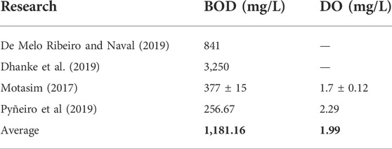
TABLE 2. BOD concentration in discharges of the shrimp industry to surface water bodies, reported in the literature.

2.6 Calibration of the dissolved oxygen model

RMSE analyzed the data set. The dissolved oxygen and BOD data calculated with the model were compared with those observed in situ and the laboratory (DO and BOD, respectively). These comparisons were made every 200 m from the point source (t = 0) for a 30-point comparison. This way, a sampling campaign was executed to calibrate the modeling results using a sensor Ezo-DO (Atlas Scientific v 5.3).

Samples for calibration and from each point source of contamination were collected according to the American Public Health Association (APHA) (1992). Each sample was analyzed for Biochemical Oxygen demand (BOD) following the technique 5210B of the same APHA (1992). The nictemeral sampling was performed with intervals of 6 h in which DO was measured in the sites indicated in Figure 1. The calculation of DO saturation for the area under study was carried out with the Henry Law employing partial pressures of Dalton. In this way, the altitude of the zone of 6 m above sea level, and the historical average of atmospheric pressure in the area of 1,005 hPa, correspond to a saturation concentration of oxygen between 7.5–9 mg/L.

2.7 Identification of anaerobic conditions in the equation of Streeter-Phelps

The point where anaerobic conditions are present is determined by Eq. 7, which considers (t) with D = O_sat. This is because if Eq. 1 is used, the deficit would be greater than the saturation oxygen, and the DO values would be negative. This phenomenon could occur in a discharge with high values of BOD, where DO could be zero.

$\left(\mathit{t}\right)=\left[\frac{{\mathit{k}}_{\mathit{d}}{\mathit{L}}_{\mathbf{0}}}{{\mathit{k}}_{\mathit{r}}{\mathit{k}}_{\mathit{d}}}\left({\mathit{e}}^{-{\mathit{k}}_{\mathit{d}}\mathit{t}}-{\mathit{e}}^{-{\mathit{k}}_{\mathit{d}}\mathit{t}}\right)+{\mathit{D}}_{\mathbf{0}}{\mathit{e}}^{-{\mathit{k}}_{\mathit{r}}\mathit{t}}\right]-{\mathit{O}}_{\mathit{s }}(7)$

DO has been wholly depleted in anaerobic conditions, and the reaction becomes zero-order (Eq. 8). Furthermore, using the initial condition of L = L_i at t = t_i, BOD in the stretch from t_i to t_f is equal to Eq. 9, indicating that BOD will decrease linearly.

$\mathit{dL}/\mathit{dt}=\mathit{ }-{\mathit{k}}_{\mathit{a}}{\mathit{O}}_{\mathit{s}}(8)$

$\mathit{L}=\mathit{ }{\mathit{L}}_{\mathit{i}}-{\mathit{k}}_{\mathit{a}}{\mathit{O}}_{\mathit{s}}\mathit{ }(\mathit{t}-{\mathit{t}}_{\mathit{i}})(9)$

Considering in Eq. 9 that, $k_r{O}_s= k_d{O}_s$, it is possible to know the endpoint of the anaerobic region (Eq. 10).

${\mathit{t}}_{\mathit{f}}={\mathit{t}}_{\mathit{i}}+\frac{\mathbf{1}}{{\mathit{k}}_{\mathit{d}}}\frac{{\mathit{k}}_{\mathit{d}}{\mathit{L}}_{\mathit{i}}-{\mathit{k}}_{\mathit{r}}{\mathit{O}}_{\mathit{s}}}{{\mathit{k}}_{\mathit{r}}{\mathit{O}}_{\mathit{s}}}(10)$

Equations 9, 10 recalculate the values of BOD and DO when values of D are higher than O_S in Eq. 1.

2.8 Future scenarios of self-depuration of Culiacan River

As stated above, by 2100 it is expected a temperature increase of up to 4°C (Guimberteau et al., 2017; Martínez-Austria et al., 2019). Changes in water temperature alter the kd constant; thus, the results obtained with the Streeter-Phelps model are affected. In order to estimate the values of kd in the future scenario, an analysis of time series for the water temperature was executed through the autoregressive integrated moving average (ARIMA). Data from CONAGUA were used (CONAGUA 2013-2020). Those analysis coincides with the IPCC reports, showing an increase of surface water of 0.9°C and forecast an increase of 1.7°C for 2100. In addition, the observed trend coincides with fluctuations in ambient temperature, for which there is a record from 1980 to 2021.

No future changes were considered for constant kr. The increase in precipitation can increase the flow rate; thus, this parameter would affect the Streeter-Phelps model. However, other phenomena in the Culiacan basin justify the value of kr being constant over the years. It is because severe drought in the northeast could cause negative changes in precipitation and the trends established for the Culiacan basin (IMTA 2021).

On the other hand, morphological alteration of rivers produced by soil erosion can generate changes in the flow. Furthermore, the aggradation process affects the river depth. These alterations would modify the kr equation. Nevertheless, rivers with the land-use conversion from forest to intensively agricultural, as is the case of the Culiacan River, tend to keep a stable flow in the long term. Since 92% of the area surrounding the CR is covered by agriculture, the possible variation of the parameters could be intertemporal (Wrzesiński and Sobkowiak 2018; Mendivil-Garcia et al., 2020).

In this way, the temperatures calculated to determine the constant kd in the future scenarios were determined from the expected increases in each year estimated from RCP 8.5 concerning the current temperature in the CR basin region. Within the parameters for the constant kr, those currently calculated were still considered. Once the future temperature of CR water has been determined, the sag curve was calculated considering climate change for different months for 2030, 2050, and 2100.

3 Results and discussion

3.1 Selection of temperatures for modeling dissolved oxygen

Figure 3 shows the groups of months resulting from cluster analysis by minimizing the Euclidean distances. Three groups were selected according to 0.8 of the maximum distance between groups. Multivariate analyzes such as clusters can be dissociative, as in the case of this investigation, because it involves temperature as a variable. It starts from a single group, the annual temperature until reaching the most significant number of groups possible, the months of the year. Moreover, the smaller the Euclidean distance, the greater the likelihood principle between the groups (James et al., 2017).

FIGURE 3

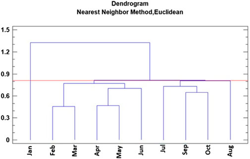
FIGURE 3. Dendrogram graphic obtained using the nearest neighbor method with Euclidean distance for the months grouping by water temperature similarity.

The above could suggest that a distance of 0.45 would arrange the months into six groups. Statistically, it would seem a better selection of the multivariate analysis because it is based on maximum homogeneity in each one. However, it was decided to maintain three groups, as shown in Figure 2, to observe the complete linkage (farthest neighbor). When using 0.45, it was observed that the distance between some groups was 0.2. In addition, the meteorological aspects of the geographical region indicate the presence of the climatic season’s winter, spring, and summer, the three groups obtained with the selected cluster analysis.

Thus, group 1 includes the months February, March, April, May, and June, which presented the warmest temperatures in the year with an average value of 25.7°C with maximum and minimum of 27.8 and 21.7°C, respectively. Group 2 includes July, August, September, and October, with the year’s highest temperatures with an average temperature of 29°C, a minimum of 25.2°C, and a maximum of 32°C. Finally, the third group includes January, the month with the lowest water temperature record, with an average temperature of 19.8°C, a minimum of 17.7°C, and a maximum of 22°C. November and December do not appear in the arrangement because the National Water Commission of Mexico does not monitor those months for the study area.

Despite the proximity between the sampling sites, a difference up to 1.6°C was observed during January. Considering that the effect of temperature on DO in rivers with pollutant discharges is exponential, the variations observed can be ecologically significant, as discussed in the following sections (Table 3).

TABLE 3

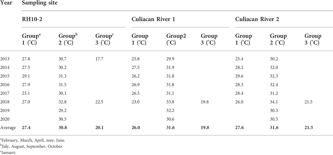
TABLE 3. Average water temperature at sites of the study transect.

3.2 Calculation of deoxygenation, k_d and reaeration k_r constants

The kd was calculated for each group of months previously obtained (Table 4). Values obtained were significantly different (p = 0.009). For groups 1, 2 and 3, were 0.30 d⁻¹, 0.36 d⁻¹ respectively. The values obtained for groups 1 and 2 are like those reported for tropical environments, with values of 0.56 ± 0.32 d⁻¹, with average temperatures of 24°C and seasonal differences derived from rainfall (Nuruzzaman et al., 2018). The kd obtained for group 3 (0.22 d⁻¹), corresponding to January, was the lowest. This value indicates a lower activity of microorganisms decomposing the organic matter as compared to the other months.

TABLE 4

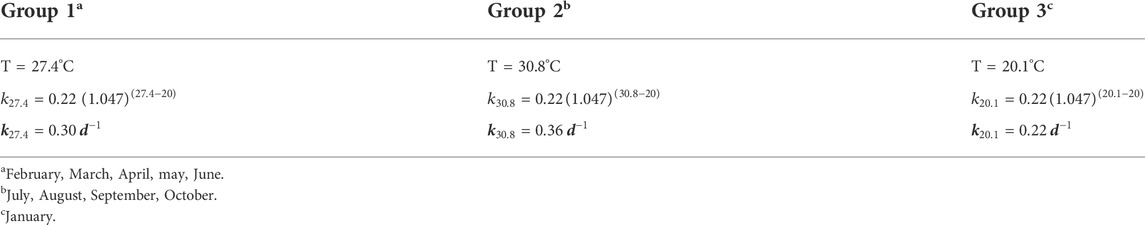
TABLE 4. Calculation of the k_d constant for the three Groups identified.

The low temperature severely inhibits the microbial activity since most heterotrophic microorganisms responsible for transforming dissolved organic matter to CO₂ are mesophilic, with an optimal metabolism at temperatures between 20–35°C. Therefore, there are the minimum acceptable conditions to biodegrade the organic matter and nutrients (Yustiani et al., 2018; Zhou et al., 2018).

To calculate the representative values of kr, the characteristics of each group obtained in Figure 3 were considered. Unlike kd, the factors determining the kr value are depth and velocity. As mentioned, the river’s depth does not vary in the selected transect (Rentería-Guevara et al., 2019). However, there is precipitation variability between groups obtained in Figure 3. Specifically, group 2 includes the months of the rainfall cycle in the region (July-October). In this geographical region, rainfall ranges between 400 and 500 mm, which implies considerable increases in the downstream flows (INEGI 2019a). Thus, since the cross-section of the CR has not undergone modifications, the increase in the flow implies an increase in current velocity, directly influencing the kr since this variable is a function of the velocity.

The flow and current velocity were calculated for each group, and subsequently, the representative kr was calculated for each group of months identified in the study area. In supplementary materials, Table 5 shows the annual upstream flow to the selected transect provided by CONAGUA and the reaeration constant in the delimited transect for each group studied. The highest reaeration rates were observed for groups 1 and 2, with 0.37 and 0.38 d⁻¹, respectively, while in January, the rate was 0.27 d⁻¹. Indeed, it is the month with the lowest flow. Streams with velocities between 0.1 and 1 m/s depend entirely on rainfall to increase the river flow rate, as is the case of the CR transect during January (CONAGUA 2019).

TABLE 5

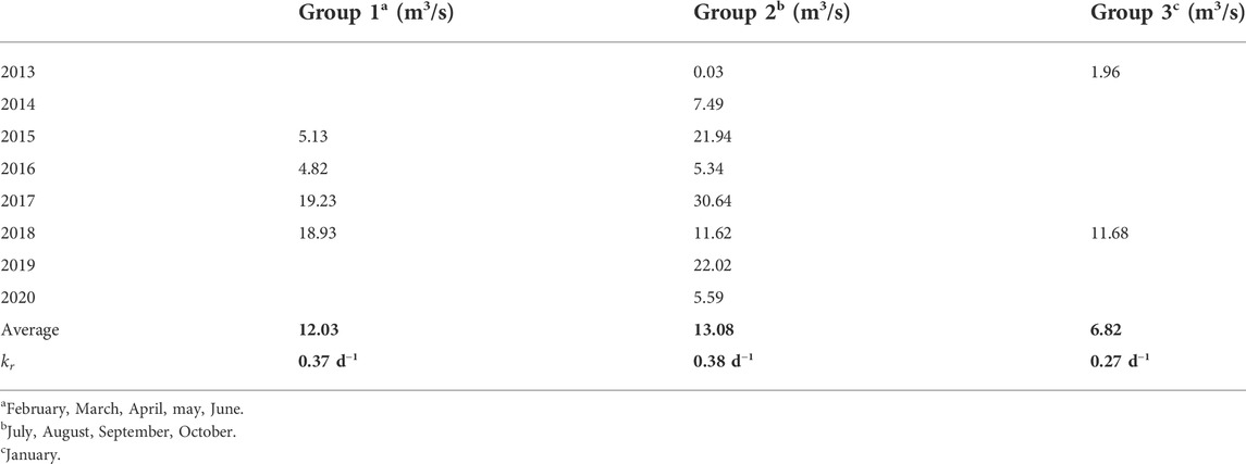
TABLE 5. Annual flow of the Cul_R lower basin and reaeration constant, k_r, for the groups studied.

In hydrological basins with tropical and subtropical climates, the highest flows occur at the end of the rainy season and during winter due to the hydraulic retention time from the upper basin to the river mouth. These values prevail for up to 4 months because of the infiltration phenomena, the aquifer recharge, and water retention typical of forests and lowland forests (Jiang et al., 2017). However, the low flow of the CR is different from other basins, where flows are higher in winter than in summer (Ali et al., 2019). This phenomenon is because the loss of vegetation cover due to the erosion caused by agricultural activity adjacent to the river (Mendivil-García et al., 2020) affects the CR capacity to concentrate surface runoff during rainfall cycles (INEGI 2019b). This change in the hydrological system of the river causes a shorter retention time than those of basins where the erosion is not significant and translates into an increase in the river flow due to the scarce winter rainfall and agricultural runoff.

3.3 Levels of dissolved oxygen and organic matter in the river before discharge

Based on the parameterization, it was observed that the CR has average DO values, recorded in the data set, of 7.36 mg/L for the months of February-June, 6.33 for July-October, and 11.08 in January. The DO saturation for the geographic area and null salinity levels of the river is, on average, 7.7 mg/L for most of the year. The flow of 13.08 m³/s is low compared to other rivers in similar regions, which would suggest oxygen levels below saturation and thus increased vulnerability (Audet et al., 2019). The DO of CR is lower than the values reported in other agricultural basins with similar climate conditions (7.85–9.98 mg/L) (South et al., 2019). In the area studied, this phenomenon could be attributed to the numerous pieces of hydraulic infrastructure along the river length, mainly irrigation canals for crops (IMTA 2018). This situation is not observed in hydrological basins with agricultural activity in countries that use technician groundwater irrigation systems or productive rainfall cycles (Reba and Massey 2020).

On the other hand, group 2 (July to October) has the lowest DO concentration, 6.33 mg/L, which is related to the high temperatures recorded in the area (up to 36°C), causing a lower DO solubility in the river. This aspect is relevant because it generates a more significant deficit before discharge (Irby et al., 2018). Also, the highest flow occurs during the months of group 2. The increase in flow is related to the annual cycle of rainfall in the Region (June to October). As mentioned in section 3.2, short-duration rainfall is characteristic in the zone because of the level of erosion observed in the CR basin since the 1990s (SEMARNAT 2021).

Regarding the concentrations of BOD, the values calculated range between 2.6 and 3.2 mg/L. The CR receive numerous wastewater discharges in the middle and lower basin. However, up to 6 km before the river mouth (just before mixing with the discharges identified in the selected transect), the river water quality can be considered “good” because BOD values are less than 6 mg/L (SEMARNAT 2008). This fact may be due to the recovery and reaeration capability of the upstream water more than the absence of polluting sources. It is essential to mention that the CR flows are 1.56 m³/s before reaching the last section of the lower basin, and at this point, the slope has decreased. The present study becomes more relevant as it is delimited to the area with the highest number of discharges from stationary sources and coincides with the river mouth into the Ensenada-El Pabellon lagoon system, classified as a RAMSAR site (RAMSAR 1999).

3.4 Modeling of dissolved oxygen in the Culiacan River

Based on the explanation in the previous Sections 3.1–3.3, Table 6 shows the final parameterization of the dissolved oxygen model in each of the three groups of months studied. For groups 1 and 2, there is a second discharge as a point source. Figure 3 shows the DO sag curves for the three groups of months identified and the DO deficit values in each of the three identified seasons (month groups). The time and critical distance from the punctual discharge are also presented.

TABLE 6

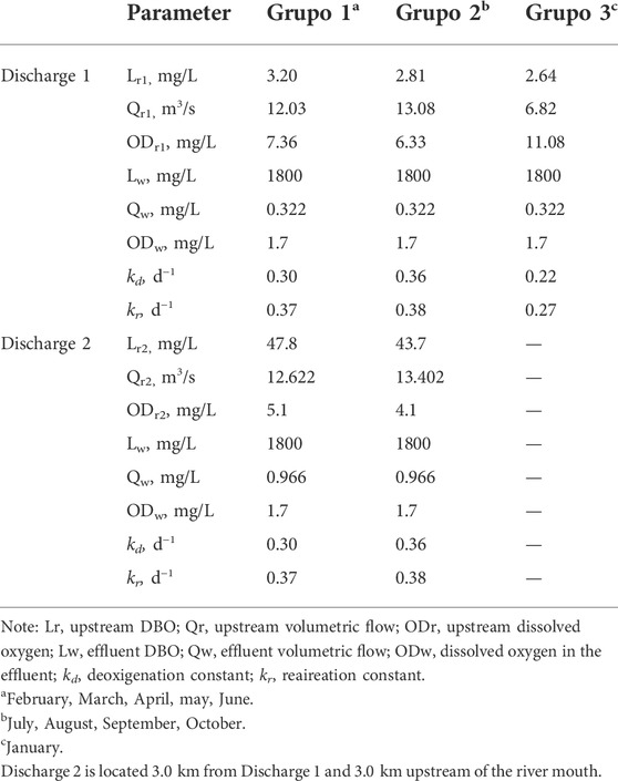
TABLE 6. Streeter-Phelps model parameters for the groups studied.

Lethal effects on fish and other aquatic organisms occur from the first hours of exposure to waters with no dissolved oxygen (Anusuya Devi et al., 2017). In Figure 4A, the typical DO sag-curve can be observed in the first 150 km, equivalent to 6 days from the point source, and the DO saturation concentration would be reached up to 250–350 km (equivalent to 10 days). In addition, within kilometers 46 and 85, the complete abatement of DO (anaerobic conditions) would be achieved at 37 h. Furthermore, the DO concentration would be less than 2.0 mg/L at different distances in the groups studied, for groups 1 and 2 between 2–248 km and 5–168 km for group 3. Below this oxygen concentration, prevail critical conditions for fish reproduction are related to the formation of ammonia and other toxins (Anusuya Devi et al., 2017). At DO levels below 1.5 mg/L the stress levels in fish can cause death, even if the condition is present only for hours (Abdel-Tawwab et al., 2019).

FIGURE 4

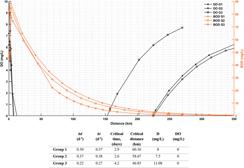
FIGURE 4. Parameter evolution in the Culiacan River after discharges; a DO as a distance-dependent function and b BOD as a distance-dependent function.

The long-distance and time required for the CR to recover its oxygen saturation levels after the discharge of wastewater are of great concern in hydrological basins since other discharges into the river could occur before recovering acceptable DO levels for aquatic organisms. Despite the analysis of the DO sag-curve for 350 km after the first wastewater discharge, the CR ends 6 km, where the river flows into a coastal lagoon system, wetland type. Figure 4 indicates that the coastal lagoon water contains high levels of organic matter (80 mg/L) that require DO to promote aerobic biodegradation. In each case study, the river water inflows with a deficit equal to the saturation value.

Coastal lagoons are lentic water bodies with low resilience capability compared to rivers. Indeed, occasional local reports of algal growth and undesirable odor production in the lagoon have been observed from time to time. Moreover, in the lagoon has been reported the loss of species during the growth phase, such as mollusks (Ostreidae) (Figure 5). Hence it is expected that the trophic level of the lagoon will gradually increase.

FIGURE 5

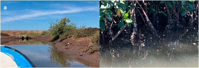
FIGURE 5. (A) Shrimp farm pond grainage; (B) mangrove near drain with oysters in growth stage.

Figure 4 shows that wastewater would have a high negative impact when discharged into the river during all months if the river were to extend beyond 6 km, even with only one discharge in group 3 (January). Indeed, anaerobic conditions would prevail for more than 150 days during the year, and the BOD values would be practically the same.

Table 6 indicates that the DO saturation level in January is 11.08 mg/L; which id 3.5 mg/L more than the values of the other groups. However, the kinetic constants kr and kd are lower during January. The kr value can be attributed to the low flow and current velocity derived from the hydrological cycle and the loss of vegetation cover in the basin. The kd is inversely proportional to temperature; it refers to bacterial catabolism. Therefore, it is equivalent to the biodegradation rate.

Indeed, the relationship between temperature and microbial activity has been extensively studied as it also impacts pollutant removal efficiency in lotic water bodies (Song et al., 2019). For instance, a null nitrification rate is observed at low temperatures (<10°C) since the growth and activity of nitrifying bacteria are considerably reduced. This phenomenon implies that, despite adequate DO levels, nitrifying bacteria cannot oxidize ammoniacal nitrogen (Li et al., 2019). The regional agricultural cycle coincides with the periods of lower temperatures, indicating a combined impact with the organic matter from the different point sources, hencecausing a drastic drop in DO concentrations.

Regarding the resilience capability of the CR, considering the transect, Figure 6 shows the DO level at the 6 km after the first discharge. The DO drops rapidly, and in January (group 3), the decrease is more abrupt, although with less magnitude, due to only a one-point source. The DO and BOD values are displayed every km from discharge to lagoon. At 3.2–3.7 km downstream of the first discharge, the DO value is close to 5 mg/L during the months of groups 1 and 3 (Supplementary Appendix S10, Supplementary Table S8). That DO value is the limit specified by the Ecological Criteria for Water Quality in Mexico (SEMARNAT 2008). This limit is reached for group 2 (July-October) at a shorter distance, 1.5 km downstream from the discharge.

FIGURE 6

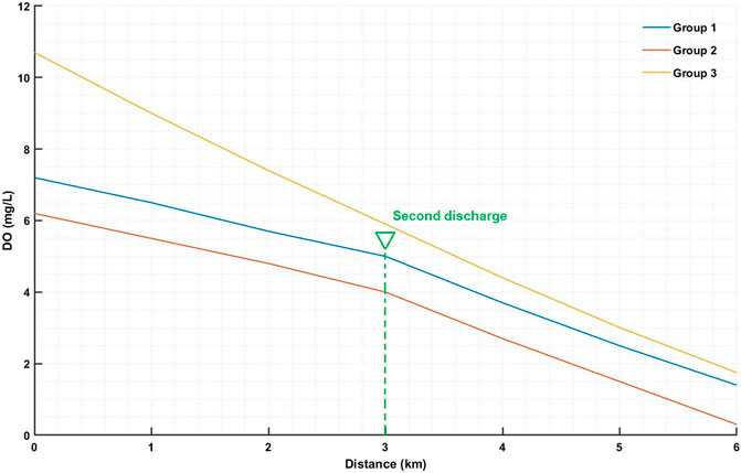
FIGURE 6. BOD values distribution in the 6 km transect downstream first point source pollution.

DO levels below 5 mg/L are of concern and represent a risk for some species of economic importance to the region, such as bivalve mollusks and shrimps. When exposure to these levels of DO is prolonged (scale of hours), the effects are lethal (Tang et al., 2020). Another species of economic importance is the largemouth bass M. Salmoides, which does not survive at concentrations lower than 3.5 mg/L for 24 h (SADER 2014). These species accounted for 33% of exports in the Pacific, and the other percentage is for national supply (PROFEPA 2010). These adverse DO conditions are reached in the CR during month groups 1 and 2 (9 months of the year) at only 0.45 km downstream from the second-point source (3.45 km from the first-point source and 2.55 km upstream from the lagoon).

At 6.0 km from the first discharge (3.0 km from the second discharge), at the mouth of the bay, the DO concentrations drop to 1.4 mg/L and 0 mg/L for the months of groups 1, 2 respectively. For group 3 (January), the DO concentration drops to 1.7 mg/L from the first discharge. These DO values cause limitations in locomotion and reproduction of freshwater fish (Roman et al., 2019). These oxygen levels also affect fish reproduction, specifically, the embryos do not fully develop in hypoxic areas, and in many cases, the eggs do not hatch (Tang et al., 2020).

The Streeter-Phelps model was used to determine the maximum organic matter level in the river discharges in a complementary way. The information obtained is essential for implementing low-cost biological treatment systems to reduce 100 mg/L BOD levels. The treatment would guarantee adequate conditions for aquatic life according to the morphological and hydrological characteristics of the river. The regulations establish limits of 30 mg/L of BOD monthly average and 60 mg/L daily average or the equivalent COD.

3.5 Future scenarios for 2030, 2050 and 2100

As mentioned in previous sections, it was observed that the high impact on the water quality of the CR occurred in all climatic seasons. In winter, it is mainly because the biodegradation rate by microorganisms, directly proportional to temperature, is limited. The effect of climate change in the area studied increases the temperature, consequently increasing the CR water’s temperature. In the remaining months of the year (groups 1 and 2), the impact is clearly due to the second point source before the system can recover from the first wastewater discharge.

Figure 7 shows the sag curve for the groups of months studied in the future scenarios of 2030, 2050, and 2100. It can be observed that the kd tends to increase in the three scenarios. For 2030, no variation is observed in the deoxygenation constant, kd, compared to 2020. This is because the increase in water temperature expected for this scenario is insignificant in 2020. According to Maberly et al. (2020), the temperature increase in surface water bodies occurs at a rate of 0.45°C every 10 years; therefore, it is not enough to vary the constant kd. However, reductions in the critical distance (where the maximum deficit is found for each group) are observed.

FIGURE 7

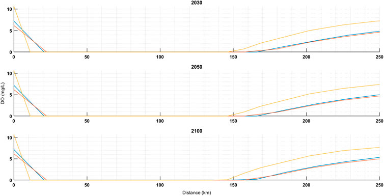
FIGURE 7. Sag curve including climate change effect for scenarios a 2030, b 2050 and c 2100.

For the 2050 scenario, changes in the deoxygenation constant were observed, increasing by 0.01 d⁻¹ in the three groups of months studied. In groups 1 and 2, a decrease of less than 1 km was observed for the critical distance (maximum DO deficit). However, in group 3, the decrease in the critical distance is up to 2.6 km compared to the 2030 scenario. In the modeling for the year 2050, a first decrease in the dissolved oxygen saturation of group 2 is observed, for the summer months, achieving a saturation and maximum DO deficit of 7.5 mg/L.

The scenario for the year 2100 for the three groups presents a significant increase in deoxygenation rates, kd. Values of 0.36, 0.42 and 0.25 d⁻¹ are for groups 1, 2 and 3 respectively. For group 2, it is observed that the estimated kd is higher than the corresponding kr value, which in ecological terms could indicate that the CR river is not resilient under these conditions.

Andrade et al. (2020) focused the study on assessing future climate change impacts on water resources of the Mundaú River Basin (MRB). Climate models predicted that the MRB will experience significant annual precipitation decreases, between 0.4% (1,087.45 mm) and 25.3% (815.59 mm). Similar behavior is expected in the Culiacan River Basin. Comparing these results with studies worldwide, the temperature presents similar increases in future scenarios using the RCP 8.5. Maximum and minimum temperature increases up to 4.3 and 2.2°C in an RCP 8.5 scenario, similar to increases expected in the Culiacan River. Compared with studies worldwide, this working temperature presents similar increases in future scenarios using the RCP 8.5.

On the other hand, Saade et al. (2021) studied the El Kalb River in a semiarid region. The study indicated that the average annual discharge of El Kalb River shortly (2021–2040) would decrease by around 28%–29% under the three RCP scenarios. End-of-century projections (2081–2100) indicated that the flow would decrease by 45% under RCP 8.5. The studies reviewed as of this present study confirm the negative impacts expected on the future climate change in the Surface water quality.

4 Conclusion

Detailed parameterization and modeling of the CR revealed that the river currently has a self-purification capability due to mechanical reaeration generated by the flow velocity, mainly in the rainy season. However, two untreated wastewater discharges occur only 6 km upstream from the river mouth.

These discharges cause a critical distance (maximum deficit) right at the river mouth. At this point, the DO can drop to 0 mg/L. Hence anoxia levels are impacting the lagoon system and endangering the ecosystem. In the case of winter season, represented by January, the river’s self-purification capability is considerably lower than the rest of the year. The constant removal of organic matter (deoxygenation) is limited by temperatures lower than 22°C. However, currently, there is only a one-point source, which allows oxygen levels not to drop to anoxic conditions. Nevertheless, less than 4.0 mg/L is reached before the river mouth, which is harmful to aquatic life.

In future scenarios, the conditions of the CR are not favorable. The increase in temperature generated by climate change has a strong negative impact, especially from July to October. During the region’s hottest months of the year, the temperature increase reduces the saturation of dissolved oxygen in the body of water, which also translatd into vulnerability to discharges of pollutants, threatening aquatic life.

Among the implications of this study, environmental and public policies are of special impact and interest. In the first implication, the model can identify ecological risks from economic activities such as aquaculture and seafood processing. On the other hand, the information would promote the development of public policies that help conserve the river facing the imminent increase in temperature caused by climate change. The primary mitigation measure recommended is the implementation of treatment systems to reduce the levels of organic matter in waters (to 100 mg/L of BOD) before discharge into the CR. Finally, limnological studies in the lagoon system are recommended since low to null levels of DO could impact the trophic level of the lagoon.

5 Limitations and future scope

Within the limitations of the research, there was the lack of availability of historical data that would have allowed expanding the field of action of the investigation. However, the future study is proposed coupling advanced dissolved oxygen models such as SWAT and QUAL2K to determine the effect of diffuse sources of pollution.

Data availability statement

The original contributions presented in the study are included in the article/Supplementary Materials, further inquiries can be directed to the corresponding author.

Author contributions

All authors contributed to the study conception and design. Material preparation, data collection and analysis were performed by KM-G, MF-D, and LA-S. The first draft of the manuscript was written by MS-J, AP-E, and AR-S. AR-M, LA-S, and AR-S evaluated the calibration of the models. All authors commented on previous versions of the manuscript. All authors agree to be accountable for the content of the work.

Funding

This work was supported by the National Council for Science and Technology (CONACYT). Grant number [633513]. The first and third authors are also grateful for the support of PAPIIT project IA107020.

Acknowledgments

The authors would like to thank CONAGUA for providing the historical water quality data for the Culiacan River.

Conflict of interest

The authors declare that the research was conducted in the absence of any commercial or financial relationships that could be construed as a potential conflict of interest.

Publisher’s note

All claims expressed in this article are solely those of the authors and do not necessarily represent those of their affiliated organizations, or those of the publisher, the editors and the reviewers. Any product that may be evaluated in this article, or claim that may be made by its manufacturer, is not guaranteed or endorsed by the publisher.

Supplementary material

The Supplementary Material for this article can be found online at: https://www.frontiersin.org/articles/10.3389/fenvs.2022.903046/full#supplementary-material

References

Abdel-Tawwab, M., Monier, M. N., Hoseinifar, S. H., and Faggio, C. (2019). Fish response to hypoxia stress: Growth, physiological, and immunological biomarkers. Fish. Physiol. Biochem. 45, 997–1013. doi:10.1007/s10695-019-00614-9

PubMed Abstract | CrossRef Full Text | Google Scholar

Ali, R., Kuriqi, A., Abubaker, S., and Kisi, O. (2019). Long-term trends and seasonality detection of the observed flow in yangtze river using mann-kendall and sen’s innovative trend method. Water 11, 1855. doi:10.3390/w11091855

CrossRef Full Text | Google Scholar

Andrade, C., Montenegro, S., Montenegro, A., Lima, J., Srinavasan, R., Jones, C., et al. (2020). Climate change impact assessment on water resources under RCP scenarios: a case study in Mundaú River basin, northeastern Brazil. Int. J. Climatol. 41, E1045–E1061. doi:10.1002/joc.6751

CrossRef Full Text | Google Scholar

Anusuya Devi, P., Padmavathy, P., Aanand, S., and Aruljothi, K. (2017). Review on water quality parameters in freshwater. Int. J. Appl. Res. 3, 114–120.

Google Scholar

APHA (1992). Standard methods for the examination of water and wastewater. Washington.

Google Scholar

Arifin, A., Mohamed, R. M. S. R., Al-Gheethi, A., Kassim, A. H. M., and Yaakob, M. A. (2019). Assessment of household greywater discharge from village houses using Streeter–Phelps model in stream. Desalination Water Treat. 179, 8–18. doi:10.5004/dwt.2020.24995

CrossRef Full Text | Google Scholar

Audet, L., Duchesne, S., and Kokutse, N. (2019). A regionalized river Water quality model calibration method based on watershed physical characteristics: application to the cau River in vietnam. rseau. 31, 251–269. doi:10.7202/1054306ar

CrossRef Full Text | Google Scholar

Benedini, M., and Tsakiris, G. (2013). Water quality modelling for rivers and streams. Dordrecht.

Google Scholar

Bui, H. H., Ha, N. H., Nguyen, T. N. D., Nguyen, A. T., Pham, T. T. H., Kandasamy, J., et al. (2019). Integration of SWAT and QUAL2K for water quality modeling in a data scarce basin of cau river basin in vietnam. Ecohydrol. Hydrobiology 19, 210–223. doi:10.1016/j.ecohyd.2019.03.005

CrossRef Full Text | Google Scholar

Chapra, S. (2008). Surface water-quality modeling. Illionois.

Google Scholar

Codesin, (2019). Sinaloa en números: Agricultura en Sinaloa al 2019. Culiacán.

Google Scholar

Codesin, (2021). Sinaloa en números: Agricultura en Sinaloa al 2020. Available at: https://sinaloaennumeros.codesin.mx/wp-content/uploads/2021/06/Reporte-29-del-2021-de-Agricultura-en-sinaloa-2020.pdf (Accessed august 11, 2021).

Google Scholar

Conagua, (2019). Comisión nacional del Agua. Available at: https://www.gob.mx/conagua/documentos/biblioteca-digital-de-mapas (Accessed june 1, 2022).

Google Scholar

Czernecki, B., and Ptak, M. (2018). The impact of global warming on lake surface water temperature in poland-the application of empirical-statistical downscaling, 1971-2100. J. Limnol. 77, 330–348. doi:10.4081/jlimnol.2018.1707

CrossRef Full Text | Google Scholar

De Melo Ribeiro, F. H., and Naval, L. (2019). Reuse alternatives for effluents from the fish processing industry through multi-criteria analysis. J. Clean. Prod. 227, 336–345. doi:10.1016/j.jclepro.2019.04.110

CrossRef Full Text | Google Scholar

de Victorica-Almeida, J. L.Universidad Nacional Autonoma de Mexico (2003). Modelación de la producción y el decaimiento del oxígeno disuelto en embalses. iit. 4, 225–236. doi:10.22201/fi.25940732e.2003.04n4.018

CrossRef Full Text | Google Scholar

Dhanke, P., Wagh, S., and Patil, A. (2019). Treatment of fish processing industry wastewater using hydrodynamic cavitational reactor with biodegradability improvement. Water Sci. Technol. 80, 2310–2319. doi:10.2166/wst.2020.049

PubMed Abstract | CrossRef Full Text | Google Scholar

DOF (2019). Plan de manejo pesquero ecosistémico del sistema lagunar altata-ensenada del Pabellón, ubicado en los municipios de Navolato y Culiacán, del Estado de Sinaloa. Available at: https://sidofqa.segob.gob.mx/notas/5573266 (Accessed august 11, 2021).

Google Scholar

Fuller, I. C., Gilvear, D. J., Thoms, M. C., and Death, R. G. (2019). Framing resilience for river geomorphology: reinventing the wheel? River Res. Appl. 35, 91–106. doi:10.1002/rra.3384

CrossRef Full Text | Google Scholar

Guimberteau, M., Ciais, P., Ducharne, A., Boisier, J. P., Dutra-Aguiar, A. P., Biemans, H., et al. (2017). Impacts of future deforestation and climate change on the hydrology of the Amazon basin: a multi-model analysis with a new set of land-cover change scenarios. Hydrol. Earth Syst. Sci. 21, 1455–1475. doi:10.5194/hess-21-1455-2017

CrossRef Full Text | Google Scholar

Häder, D.-P., and Barnes, P. W. (2019). Comparing the impacts of climate change on the responses and linkages between terrestrial and aquatic ecosystems. Sci. Total Environ. 682, 239–246. doi:10.1016/j.scitotenv.2019.05.024

PubMed Abstract | CrossRef Full Text | Google Scholar

He, L., Shen, J., and Zhang, Y. (2018). Ecological vulnerability assessment for ecological conservation and environmental management. J. Environ. Manage. 206, 1115–1125. doi:10.1016/j.jenvman.2017.11.059

PubMed Abstract | CrossRef Full Text | Google Scholar

IMTA (2018). Análisis comparativo de la operación del Distrito de Riego 010 Culiacán-Humaya en seis ciclos agrícolas. Aguascalientes: Instituto Mexicano de Tecnología del Agua. Available at: https://www.riego.mx/congresos/comeii2018/assets/ponencias/presentacion/18021.pdf (Accessed september 16, 2021).

Google Scholar

IMTA (2021). Perspectiva sobre la sequía actual en México. Aguascalientes: Instituto Mexicano de Tecnología del Agua. Available at: https://www.gob.mx/imta/es/articulos/perspectiva-sobre-la-sequia-actual-en-mexico?idiom=es (Accessed july 20, 2021).

Google Scholar

INAPESCA (2019). Plan de Manejo Pesquero Ecosistémico del sistema lagunar Altata-Ensenada del Pabellón en el estado de Sinaloa. Mexico City: Instituto Nacional de Pesca. Instituto Nacional de Pesca. Available at: https://www.gob.mx/inapesca/prensa/establece-sader-plan-de-manejo-pesquero-ecosistemico-del-sistema-lagunar-altata-ensenada-del-pabellon-en-el-estado-de-sinaloa july 13, 2021).

Google Scholar

INEGI (2021). Censo de Población y vivienda 2020. Instituto Nacional de Estadística y Geografía. https://www.inegi.org.mx/programas/ccpv/2020/#Datos_abiertos (Accessed april 13, 2021).

Google Scholar

INEGI (2019a). Cuenca hidrológica río culiacán: Humedales, méxico. Aguascalientes. México.

Google Scholar

INEGI (2019b). instituto nacional de Estadística y geografía. Available at: https://www.inegi.org.mx/contenido/productos/prod_serv/contenidos/espanol/bvinegi/productos/nueva_estruc/702825190934.pdf (Accessed april 3, 2021).

Google Scholar

IPCC (2019). “Global Warming of 1.5°C. An IPCC Special Report on the impacts of global warming of 1.5 °C above pre-industrial levels and related global greenhouse gas emission pathways,” in The context of strengthening the global response to the threat of climate change, sustainable development, and efforts to eradicate poverty (Geneva: Press).

Google Scholar

Irby, I., Friedrichs, M., Da, F., and Hinson, K. (2018). The competing impacts of climate change and nutrient reductions on dissolved oxygen in Chesapeake Bay. Biogeosciences 15, 2649–2668. doi:10.5194/bg-15-2649-2018

CrossRef Full Text | Google Scholar

James, G., Witten, D., Hastie, T., and Tibshirani, R. (2017). “Unsupervising learning,” in An introduction to statistical learning. Editors C. G, S. Fienberg, and I. Olkin (New York: Springer), 373.

Google Scholar

Jiang, C., Liu, Y., Long, Y., and Wu, C. (2017). Estimation of residence time and transport trajectory in tieshangang bay, China. Water 9, 321. doi:10.3390/w9050321

CrossRef Full Text | Google Scholar

Kamal, N. A., Muhammad, N. S., and Abdullah, J. (2020). Scenario-based pollution discharge simulations and mapping using integrated QUAL2K-GIS. Environ. Pollut. 259, 113909. doi:10.1016/j.envpol.2020.113909

PubMed Abstract | CrossRef Full Text | Google Scholar

León-Cortés, J. L., Gómez-Velasco, A., Sánchez-Pérez, H. J., Leal, G., and Infante, F. (2018). La salud ambiental: algunas reflexiones en torno a la biodiversidad y al cambio climático. Rev. Enferm. Emerg. 17, 26–36.

Google Scholar

Li, C., Liu, S., Ma, T., Zheng, M., and Ni, J. (2019). Simultaneous nitrification, denitrification and phosphorus removal in a sequencing batch reactor (SBR) under low temperature. Chemosphere 229, 132–141. doi:10.1016/j.chemosphere.2019.04.185

PubMed Abstract | CrossRef Full Text | Google Scholar

Maberly, S. C., O’Donnell, R. A., Woolway, R. I., Cutler, M. E. J., Gong, M., Jones, I. D., et al. (2020). Global lake thermal regions shift under climate change. Nat. Commun. 11, 1232. doi:10.1038/s41467-020-15108-z

PubMed Abstract | CrossRef Full Text | Google Scholar

Martínez Austria, P. F., Díaz-Delgado, C., and Moeller-Chavez, G. (2019). Seguridad hídrica en méxico: diagnóstico general y desafíos principales. Ing. Agua 23, 107. doi:10.4995/ia.2019.10502

CrossRef Full Text | Google Scholar

Mendes, S. A., Gonçalves, E. V., Frâncica, L. S., Correia, L. B. C., Nicola, J. V. N., Pestana, A. C. Z., et al. (2020). Quality of natural waters surrounding campo mourão, state of paraná, southern Brazil: Water resources under the influences from urban and agricultural activities. Water Air Soil Pollut. 231, 415. doi:10.1007/s11270-020-04795-5

CrossRef Full Text | Google Scholar

Mendivil-Garcia, K., Amabilis-Sosa, L. E., Rodríguez-Mata, A. E., Rangel-Peraza, J. G., Gonzalez-Huitron, V., Cedillo-Herrera, C. I. G., et al. (2020). Assessment of intensive agriculture on water quality in the Culiacan River basin, Sinaloa, Mexico. Environ. Sci. Pollut. Res. 27, 28636–28648. doi:10.1007/s11356-020-08653-z

PubMed Abstract | CrossRef Full Text | Google Scholar

Nuruzzaman, M., Al-Mamum, A., and Salleh, M. (2018). Experimenting biochemical oxygen demand decay rates of malaysian river water in a laboratory flume. Environ. Eng. Res. 23, 99–106. doi:10.4491/eer.2017.048

CrossRef Full Text | Google Scholar

Paudel, J., and Crago, C. L. (2021). Environmental externalities from agriculture: evidence from water quality in the united states. Am. J. Agric. Econ. 103, 185–210. doi:10.1111/ajae.12130

CrossRef Full Text | Google Scholar

Pesce, M., Critto, A., Torresan, S., Giubilato, E., Santini, M., Zirino, A., et al. (2018). Modelling climate change impacts on nutrients and primary production in coastal waters. Sci. Total Environ. 628, 919–937. doi:10.1016/j.scitotenv.2018.02.131

PubMed Abstract | CrossRef Full Text | Google Scholar

Profepa, (2010). Biblioteca de Publicaciones Oficiales del Gobierno de México. Mexico City. Available at: https://www.profepa.gob.mx/innovaportal/v/3274/1/mx.wap/lista_flota_camaronera_mexicana_para_exportar_a_estados_unidos.html (Accessed september 29, 2021).

Google Scholar

Pyñeiro, M., Chalar, G., and Quintans, F. (2019). Constructed wetland scale model: organic matter and nutrients removal from the efuent of a fsh processing plant. Int. J. Environ. Sci. Technol. 16, 4181

Google Scholar

Quiroz-Fernández, L. S., Izquierdo-Kulich, E., and Menéndez-Gutiérrez, C. (2018). Estudio del impacto ambiental del vertimiento de aguas residuales sobre la capacidad de autodepuración del río Portoviejo, Ecuador. Cent. Azúcar 45, 73–83.

Google Scholar

RAMSAR (1999). Ficha Informativa de los humedales de ramsar. ramsar. Available at: https://rsis.ramsar.org/RISapp/files/RISrep/MX1340RIS.pdf (Accessed september 17, 2021).

Google Scholar

Reba, M. L., and Massey, J. H. (2020). Surface irrigation in the lower mississippi river basin: trends and innovations. Trans. ASABE 63, 1305–1314. doi:10.13031/trans.13970

CrossRef Full Text | Google Scholar

Rentería-Guevara, S. A., Rangel-Peraza, J. G., Rodríguez-Mata, A. E., Amábilis-Sosa, L. E., Sanhouse-García, A. J., Uriarte-Aceves, P. M., et al. (2019). Effect of agricultural and urban infrastructure on river basin delineation and surface water availability: case of the culiacan river basin. Hydrology 6 (3), 58. doi:10.3390/hydrology6030058

CrossRef Full Text | Google Scholar

Rodríguez, F. S. S. (2020). Los impactos del cambio climático en la gestión del agua en la Ciudad de México Argumentos. Estudios críticos de la sociedad, 81–102. doi:10.24275/uamxoc-dcsh/argumentos/202092-04

CrossRef Full Text | Google Scholar

Roman, M., Brandt, S., Houde, E., and Pierson, J. (2019). Interactive effects of hypoxia and temperature on coastal pelagic zooplankton and fish. Front. Mar. Sci. 6, 39. doi:10.3389/fmars.2019.00139

CrossRef Full Text | Google Scholar

Saade, J., Athied, M., Ghanimeh, S., and Golmohammadi, G. (2021). Modeling impact of climate change on surface water availability using SWAT model in a semi-arid basin: Case of el Kalb River, Lebanon. Hydrology 8, 134. doi:10.3390/hydrology8030134

CrossRef Full Text | Google Scholar

SADER (2014). Catalogo de peces. Guadalajara: Agricultura y Desarrollo rural. Available at: https://sader.jalisco.gob.mx/catalogo-peces/lobina#:∼:text=Para%20su%20desarrollo%20se%20necesita,disuelto%20mayor%20a%204%20ppm (Accessed october 9, 2021).

Google Scholar

Semarnat, (2008). Compendio de estadísticas ambientales. Mexico City: Secretaria de Medio Ambiente y Recursos Naturales. Available at: https://apps1.semarnat.gob.mx:8443/dgeia/cd_compendio08/compendio_2008/compendio2008/10.100.8.236_8080/ibi_apps/WFServleta0c5.html (Accessed september 7, 2021).

Google Scholar

Semarnat, (2021). Compendio de estadísticas ambientales. Secretaria de Medio Ambiente y Recursos Naturales. Available at: https://apps1.semarnat.gob.mx:8443/dgeia/compendio_2021/01_ambiental/agua.html Accesed 1 june 2022.

Google Scholar

SIAP (2020). Sinaloa: Infografía agroalimentaria 2020. Mexico City: Ciudad de México.

Google Scholar

Song, H. L., Li, X. N., Lu, X. W., and Inamori, Y. (2009). Investigation of microcystin removal from eutrophic surface water by aquatic vegetable bed. Ecol. Eng. 35, 1589–1598. doi:10.1016/j.ecoleng.2008.04.005

CrossRef Full Text | Google Scholar

South, E. J., DeWalt, E., and Cao, Y. (2019). Relative importance of Conservation Reserve Programs to aquatic insect biodiversity in an agricultural watershed in the Midwest, USA. Hydrobiologia 829, 323–340. doi:10.1007/s10750-018-3842-2

CrossRef Full Text | Google Scholar

Tang, R. W., Doka, S. E., Gertzen, E. L., and Neigum, L. M. (2020). Dissolved oxygen tolerance guilds of adult and juvenile Great Lakes fish species. Ontario: Fisheries and Oceans Canada.

Google Scholar

Tehreem, H. S., Anser, M. K., Nassani, A. A., Abro, M. M. Q., and Zaman, K. (2020). Impact of average temperature, energy demand, sectoral value added, and population growth on water resource quality and mortality rate: it is time to stop waiting around. Environ. Sci. Pollut. Res. 27, 37626–37644. doi:10.1007/s11356-020-09822-w

PubMed Abstract | CrossRef Full Text | Google Scholar

Wahyuningsih, S., Novita, E., and Idayana, D. A. (2020). Penilaian daya dukung sungai antirogo di kabupaten jember terhadap beban pencemaran menggunakan metode streeter-phelps. agriTECH 40, 199. doi:10.22146/agritech.50450

CrossRef Full Text | Google Scholar

Wrzesiński, D., and Sobkowiak, L. (2018). Detection of changes in flow regime of rivers in Poland. J. Hydrol. Hydromech. 66, 55–64. doi:10.1515/johh-2017-0045

CrossRef Full Text | Google Scholar

Yang, K., Yu, Z., Luo, Y., Zhou, X., and Shang, C. (2019). Spatial-temporal variation of lake surface water temperature and its driving factors in yunnan-guizhou plateau. Water Resour. Res. 55, 4688–4703. doi:10.1029/2019WR025316

CrossRef Full Text | Google Scholar

Yustiani, Y. M., Nurkanti, M., Suliasih, N., and Novantri, A. (2018). Influencing parameter of self purification process in the urban area of cikapundung river, indonesia. Int. J. Geomate 14, 50–54. doi:10.21660/2018.43.3546

CrossRef Full Text | Google Scholar

Zhou, H., Li, X., Xu, G., and Yu, H. (2018). Overview of strategies for enhanced treatment of municipal/domestic wastewater at low temperature. Sci. Total Environ. 643, 225–237. doi:10.1016/j.scitotenv.2018.06.100

PubMed Abstract | CrossRef Full Text | Google Scholar