Testing a New Ensemble Vegetation Classification Method Based on Deep Learning and Machine Learning Methods Using Aerial Photogrammetric Images

The objective of this research is to report results from a new ensemble method for vegetation classification that uses deep learning (DL) and machine learning (ML) techniques. Deep learning and machine learning architectures have recently been used in methods for vegetation classification, proving their efficacy in several scientific investigations. However, some limitations have been highlighted in the literature, such as insufficient model variance and restricted generalization capabilities. Ensemble DL and ML models has often been recommended as a feasible method to overcome these constraints. A considerable increase in classification accuracy for vegetation classification was achieved by growing an ensemble of decision trees and allowing them to vote for the most popular class. An ensemble DL and ML architecture is presented in this study to increase the prediction capability of individual DL and ML models. Three DL and ML models, namely Convolutional Neural Network (CNN), Random Forest (RF), and biased Support vector machine (B-SVM), are used to classify vegetation in the Eastern part of Serbia, together with their ensemble form (CNN-RF-BSVM). The suggested DL and ML ensemble architecture achieved the best modeling results with overall accuracy values (0.93), followed by CNN (0.90), RF (0.91), and B-SVM (0.88). The results showed that the suggested ensemble model outperformed the DL and ML models in terms of overall accuracy by up to 5%, which was validated by the Wilcoxon signed-rank test. According to this research, RF classifiers require fewer and easier-to-define user-defined parameters than B-SVMs and CNN methods. According to overall accuracy analysis, the proposed ensemble technique CNN-RF-BSVM also significantly improved classification accuracy (by 4%).

1 Introduction

Forests are a valuable natural resource in many countries, with wood and forestry products serving as the primary export cheeses. They’re also crucial in water management, tourism and recreation, wildlife protection, and soil erosion control. The process of photosynthesis allows plants to play a critical role in all major planetary cycles, including water circulation in nature, energy exchange, oxygen, carbon dioxide, and other elements between biotic and abiotic regions (Drobnjak et al., 2018; Wang et al., 2021).

Satellite and aerial images are effective instruments for monitoring and studying forests and other vegetation. Satellite images are useful equipment for forest monitoring, and remote sensing research has become a very effective method. Satellite images can be used to explore the borders between different types of vegetation, the degree of vegetation development, vegetation morphology, forest health, tree canopy humidity, diverse textures, biomass, and a variety of other parameters (Drobnjak et al., 2013; Bakrač et al., 2018; Drobnjak et al., 2018).

Only radiometric, spatial, and spectrally enhanced images are suitable for further digital analysis to collect the data required for vegetation classification. Classification is the process of grouping pixels into thematic groups or classes using statistical methods and detecting the association between their digital values. It is one of the most difficult processes in computer image processing in terms of operator knowledge. In practice, classification methods entail assessing the image’s content and grouping pixels into the proper data categories (Running et al., 1995; Yu et al., 2006; Xie et al., 2008). The unification is carried out according to a predetermined numerical analysis decision rule (application of the corresponding key). This is accomplished by statistically categorizing pixels into thematic groups based on their digital values, as well as the relationship between the contents of the entities, referred to as “class” (Running et al., 1995).

The use of a combination of many classifiers to achieve a single classification has been documented in the remote sensing literature several times in recent years (Yu et al., 2006; Xie et al., 2008; Engler et al., 2013; Kussul et al., 2017; Meng et al., 2017; Amini et al., 2018; Drobnjak et al., 2018; Ayhan et al., 2020). The ensemble classifier that results is often found to be more accurate than any of the individual classifiers that make up the ensemble. To categorize unknown causes, an ensemble classifier employs weighted or unweighted voting to integrate the decisions of a group of classifiers (Dietterich, 2000; Engler et al., 2013). For vegetation classification, studies that used boosting with a decision tree as the base classifier indicated a considerable increase in classification accuracy (Chan and Paelinckx, 2008; Xie et al., 2008). In the past, the random forest (RF) algorithm has proved successful in producing realistic vegetation maps (Ghimire et al., 2010). RF has been successfully utilized to extract physiological plant features (Doktor et al., 2014), estimate plant biomass (Adam et al., 2014), and map plant species in studies using multispectral data for forest sciences (Burai et al., 2015).

SVM is frequently cited as the best method for dealing with difficult classification issues such as tree species discrimination, with RF coming in second (Ghosh et al., 2014). Ghosh et al. (2014) used information from a broader electromagnetic spectrum (450–2,500 nm) to employ SVM and RF on multispectral data to categorize five tree species in managed woods in central Germany.

The purpose of this paper is to discuss the findings obtained utilizing a combination of Random Forest, a biased Support vector machine, and a Convolutional Neural Network classifier. All mentioned classifiers use a bootstrapped sample of the training data to select a random set of features and create a classifier. This generates a large number of trees (classifiers), and then unweighted voting is used to assign an unknown pixel to a class (Shaheen and Verma, 2016; Sothe et al., 2020; Gašparović and Dobrinić, 2020; Zhang et al., 2020; Fei et al., 2022). The new ensemble classifier’s performance is also compared to that of single classifiers in terms of classification accuracy, training time, and user-defined parameters (Meng et al., 2017).

Machine learning algorithms define computer-based tools that allow for exploratory data and statistical analysis to uncover unknown patterns and relationships in dataset values ahead of time. The current study used supervised and flexible machine learning algorithms, deep learning algorithms, and their ensemble to categorize vegetation areas in the eastern part of Republic Serbia’s Suva Planina Mountain.

2 Materials and Methods

2.1 Study Area and Remote Sensed Data Acquisition

Forest area in Republic Serbia covered 27,200 km² which is approximately 31.1% of the country area. The study area includes parts of Mountain Suva Planina near Niš City, between latitudes of 43°15′15″–43°19′45″N, and longitudes of 22°20′15″–22°30′00″E. The area covered by the test area is 109.7 km². The minimum altitude of the test area is 326.4 m, the maximum altitude is 1,154.8 m, and the average altitude of the test area is 680.9 m. It is located in the eastern part of the Republic of Serbia (Figure 1).

FIGURE 1

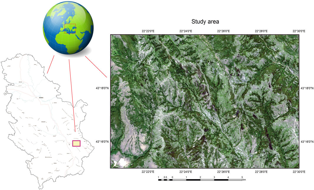
FIGURE 1. Location of the study area.

Data from the digital sensors of the satellite system Sentinel-2A and the digital aerial photogrammetric camera Leica ADS80 were used to create the combination of aerial photogrammetric and satellite images (Running et al., 1995; Amarsaikhan and Douglas, 2004).

Sentinel-2A is the first optical Earth observation sensor developed and built by Airbus (Airbus Defense and Space—ADS) for the European Space Agency’s (ESA) needs as part of the European Copernicus program (Table 1). Sentinel-2A is the first civil optical Earth observation satellite with sensors in four “Red Edge” wavelengths, which provides critical data on vegetation on the planet’s surface (Fernández-Manso et al., 2016; Mallinis et al., 2018).

TABLE 1

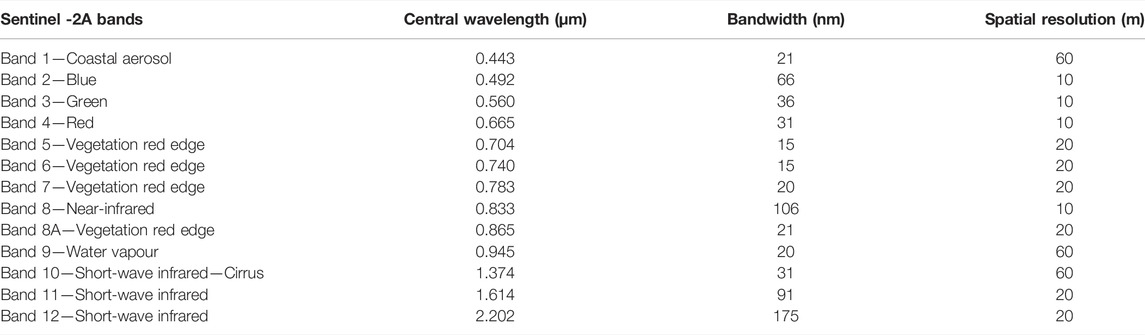
TABLE 1. Characteristics of Sentinel-2A images.

In addition, the aerial Photogrammetric Acquisition System of the Military Geographic Institute consists of airplane Piper Seneca V and digital aerial photogrammetric camera Leica ADS80 (Figure 2): The system provides a modern approach in the field of collecting and analyzing geospatial data for the needs of the defense system entities and other users in the country (Drobnjak et al., 2018).

FIGURE 2

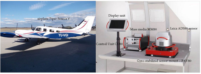
FIGURE 2. Aerial photogrammetric recording system.

In this study, we used data obtained from a multispectral sensor (panchromatic, RGB, and infrared bands)—digital camera Leica ADS80 (Drobnjak et al., 2018), which has a line sensor with a resolution of 6.5 μm, with 12,000 pixels per line or 24,000 pixels when using HiRes Mode, with Lens focus 62.7 mm. The above aerial photogrammetric images were downscaled with satellite images of the Sentinel 2A mission.

During the field research in 2020 and 2021, samples for training and testing datasets were collected. Localization of selected tree species was achieved during data collecting. Only regions currently occupied by living trees above 5 m height were deemed acceptable location sources during field data collecting. The chosen sampling sites are required to have a minimum of five trees of the same species within a 3-m radius of the GPS receiver. In this study, we used the Trimble T10 tablet GPS device which is a powerful, rugged device created for survey fieldwork, mapping, and GIS data collection and at the same time supports demanding desktop applications. Trimble T10 has Windows 10 Enterprise operating system, with a 10.1″ screen size, Intel i7 processor, internal GPS with SBAS, 8 GB memory, and 256 GB data storage.

Only measurements with a localization error of less than 1.5 m were chosen. The coordinates of polygon corners were recorded for larger areas and then used for pixel extraction. Areas that were definitely in shade and pixels that were uncertain were eliminated.

2.2 Methods

The Leica ADS80 multispectral dataset was then utilized to extract training and testing samples from these locations. Leica ADS80 capabilities include perfectly co-registered multispectral bands and true stereo image collection. The spatial resolution of the multispectral (RGB and Infrared bands) aerial photogrammetric images used in the paper was 40 cm. The flight altitude of the plane during the aerial photogrammetric scanning was 4,000 m. Using a combination of aerial photogrammetric images and satellite images, the spatial resolution was downscaled to 2.5 m. Machine and Deep learning classification methods were used on such images to create a thematic layer of vegetation.

Supervised vegetation classification consists of a training stage and an evaluation performance stage, and a confusion matrix is constructed and used for accuracy assessment. In this study, we used collected reference test samples with different NDVI indexes and different vegetation textures and shapes. Using a GIS program, we categorized the different forest types data as training and testing samples for our experimental setup. The labeled data was collected in the field, alongside additional high-resolution imagery from other datasets and imaging (both satellite and aerial). We defined a total of eight vegetation classes based on the different types of forest vegetation found in the test region and included them in the analysis. Test samples were directly mapped from aerial photogrammetric images as polygons of different dimensions and thus stored in the reference test sample database.

A total of 398 forest-type vegetation features (polygons) and 225 non-forest vegetation features (e.g., water, soil, grass, and other land coverings) were annotated on a combination of aerial and satellite photos, resulting in 623 various sizes polygons. Although the proximity of polygons makes it appear like some of them are present in both subsets, this is not the case. This happened only when small polygons were represented in the figure size because the training and testing sets had completely distinct features. We used the bootstrap technique to define the training and testing datasets to explore the performance of the machine and deep learning algorithms in the classification of forest vegetation (polygon features).

The sample size and quality of training data have generally had a large impact on the classification accuracy. In this regard, we divided the dataset while ensuring that both training and testing sets contained similar sampling patterns, being representatives of all conditions observed in the area during labeling. Using a large number of reference samples the uncertainty of the estimator can be evaluated.

Because the majority of supervised classifiers are sensitive to the data used for training, classification results will vary based on the training dataset. Furthermore, in order to exclude human bias from classification results, we chose to use a technique that included a random selection of training and testing datasets that belong to the already mentioned test sample polygons. We chose the 0.632 bootstrap strategy for producing the test and training datasets based on the work of (Ghosh et al., 2014; Neto and Dougherty, 2015).

Bootstrapping is a statistical technique for producing random samples and estimating the distribution of a population estimator using a random sample or a model estimated from a random sample (Ghosh and Prajneshu, 2011). It entails examining the data as if it were a population in order to assess the distribution of interest. When determining the asymptotic distribution of an estimator or statistic is challenging, bootstrapping can be used to replace computation with mathematical analysis.

The entire method was d divided into several iterations. Each cycle involves a random split of all samples into test and training datasets, with 63.2% of samples going to the training dataset and the rest going to the test dataset, which is not used in the classifier training process and belongs to the already mentioned test sample polygons.

Table 2 shows the exact amount of samples/pixels assigned to each class. Following this, classification was performed using the given training samples and classification method.

TABLE 2

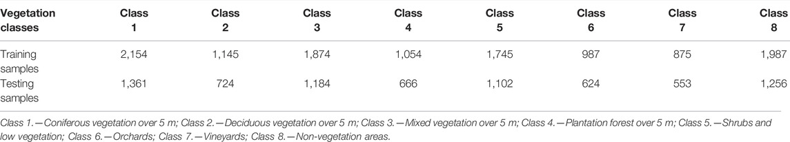
TABLE 2. Training and testing sample sizes (in pixels) used for vegetation classifications.

Figure 3 depicts the flowchart of the method utilized in the study. The dataset construction is demonstrated in the first step, where all data is entered into the database, including a combination of satellite and aerial photogrammetry photos as well as vector data of test samples. Models of biased Support vector machines, Random Forests, and Convolutional Neural Networks, as well as their ensemble classification methods, were used in the following. For this study, machine learning and deep learning classification algorithms with their ensemble classifier were evaluated through R software. Then, the precision, total accuracy, and kappa coefficient were used to validate the built models. Finally, we used the Wilcoxon Signed-Rank significance test to statistically test the proposed techniques.

FIGURE 3

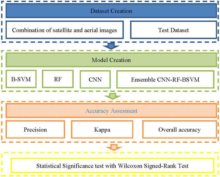
FIGURE 3. Flowchart of the used methodology in the study.

Biased Support vector machines, Random Forests, Convolutional Neural Networks, and their ensemble classification algorithms all used the same training data and were tested on the same test data, ensuring that the findings were comparable.

The next stage was to compare classifiers by analysing the differences in producer and user classification accuracy for classes, as well as the overall accuracy and kappa coefficient variability. The best (most accurate) iteration for each classification method was chosen based on the results. The final categorization images were created using the optimal iteration parameters. With the help of an NDVI-based mask, non-forested areas were masked out from the final images. To avoid the classification of bushes and young tree stands, vegetation smaller than 2 m was concealed. We achieved this by mapping and field testing test samples containing lower trees and low vegetation. Pixels having an NDVI value less than 0.25 were also masked to remove buildings and manufactured elements.

2.3 Performance Evaluation

The proportion of the total number of correctly categorized pixels across all classes and the total number of pixels in the confusion matrix is referred to as overall accuracy (the total sum of pixels divided by the sum of diagonal elements of the matrix). The errors associated with individual classes are described by User and Producer accuracies. The likelihood of a reference pixel being correctly categorized is measured by the producer’s accuracy (total number of pixels in that category determined from reference data divided by the total number of pixels in that category). The likelihood that the predicted sample class matches the reference class is the user’s accuracy (the total number of correct classifications for a particular class and dividing it by the row total).

$\mathit{\text{Overall}}\mathit{\text{accuracy}}=\frac{{{\displaystyle \sum }}_{i=1}^k{n}_{ii}}{n}\text{*}100(1)$

$\mathit{User}\text{'}\mathit{s}\mathit{\text{accuracy}}=\frac{n_{ii}}{n_{i+}}(2)$

$\mathit{Producer}\text{'}\mathit{s}\mathit{\text{accuracy}}=\frac{n_{ii}}{n_{+i}}(3)$

With the usage of the confusion matrix, we get a coefficient of kappa statistics which is a good indicator of the choice of classification method consistency taking their randomness into account. Kappa coefficient (κ) is a coefficient that quantifies the degree of compatibility between assigned classes when misclassification is removed.

In general, the kappa coefficient is being reduced with enlargement of the number of classes, i.e., the better classes are selected the greater possibility of an error in classification. Kappa coefficient is κ = 0 for the clear compatibility between the two total coincidental classifications and it reaches κ = 1 for complete harmonization between the classification and data. For unexpectedly accurate class agreement, kappa statistics are utilized as a measure of classification accuracy.

$\mathit{\text{Kap}}\mathit{\text{pacoef}}\mathit{\text{ficient}}=\frac{n{{\displaystyle \sum }}_{i=1}^k{n}_{ii}-{{\displaystyle \sum }}_{i=1}^k{n}_{i+}{n}_{+i}}{n^2-{{\displaystyle \sum }}_{i=1}^k{n}_{i+}{n}_{+i}}(4)$

With a random distribution of pixels in the classes, the registered value indicates the overall classification accuracy and consistency between the image and the reference grid. According to Landis and Koch (Landis and Koch, 1977), values of Kappa coefficient greater than 0.8 indicate perfect agreement, values between 0.6 and 0.8 indicate substantial agreement, values between 0.4 and 0.6 indicate moderate agreement, and values between 0.2 and 0.4 indicate fair agreement, and values below 0.2 indicate poor agreement. Furthermore, to compare the classification performances of the ML, DL, and their ensemble models, a statistical significance test (Wilcoxon signed-rank test) is used (Woolson, 2008). The Wilcoxon signed-ranked test, a nonparametric hypothesis test, is used to statistically evaluate the efficacy of the models developed. The test has been widely used to determine the statistical significance of performance differences between models and to compare them pair-wise (Woolson, 2008). The Wilcoxon signed-rank test’s null hypothesis is that there is no statistical difference between the models at a 95% confidence range. By using Wilcoxon signed-rank test we calculate how far each value of the producer’s accuracy, user’s accuracy, and the overall accuracy of individual classes is from the hypothetical median. Wilcoxon signed-rank test p-values of the producer’s accuracy, user’s accuracy, and the overall accuracy of individual classes were greater than 0.05 which proves there is no statistical difference between the models at a 95% confidence range.

3 Machine and Deep Learning Applications

3.1 Machine Learning Classification

Machine learning technique emerged as a response to the rigidity of many computer programs in comparison to the unlimited variability of the environment. One of the most difficult aspects of feature detection from remote sensing images has been accurately distinguishing real-world objects from a vast number of pixels. Machine learning is a branch of computer science that studies algorithms that learn from examples. Classification is a task that necessitates the application of machine learning algorithms to learn how to assign a class label to problem domain instances. In machine learning, there are many distinct sorts of classification tasks to be encountered and specialized modeling approaches to be employed for each.

3.1.1 Biased Support Vector Machine Techniques

The support vector machine (SVM) is a commonly used statistical machine learning technique that works on the premise of risk minimization. The support vector machine approach divides the classes using a final surface (referred to as an ideal hyper-plane) that maximizes the margin between the classes in the dataset. In the same way that a regular binary SVM determines the best separation between two classes in feature space, a biased SVM does the same. The acquired training data from the focal class, on the other hand, is compared against samples taken at random from the data pool (in this case, the vegetation pixels from the entire island), which are referred to as “pseudo-outliers” in this context (Chan and King; Hartono et al., 2018). Because the pseudo-outlier data has no known identity and will comprise samples from the focus class, errors in the pseudo-outlier class are penalized less severely than errors in the focal class.

Furthermore, the standard SVM approach makes two assumptions: the positive and negative training samples are of equal size, and the cost of misclassification for samples belonging to various classes is essentially the same. For positive and negative samples, the Biased-SVM method is used to apply various penalty coefficients C. In this algorithm, the minority samples are given higher penalty factors, while the majority samples are given lower penalty factors. As a result, the SVM classifier can concentrate on the minority class’s misclassification rate.

Assuming that $D=\left\{\left(x_i,y_i\right)\right\}\left(1\le i\le n\right)$ is the training set, where $x_i$ denotes the feature vector of $\mathit{P}i$ and $y_i\in \{-1, 1\}$ is the label of $\mathit{P}i$, the first verified parts are $m - 1$ and they are positive examples labeled as $y_i = 1(1 \le i \le m - 1)$, while the rest are unlabeled part whose labels are set to $y_i = -1(m \le i \le n)$. Furthermore, two soft margin parameters, $C_1$ and $C_2$, are included to highlight the differing tolerances on the training mistakes induced by positive and unlabeled octapeptides, respectively (Foody and Mathur, 2004; Hartono et al., 2018; Li et al., 2021). These two factors can likewise be used to learn from a noisy unlabeled collection with cleaved sections. The two L1-norm soft margins biased formulation of SVM is described by Eq. 5:

$\mathit{\text{Minimize}}: \frac{1}{2}{\omega }^t\omega +C_1{\displaystyle \sum }_{i=1}^{m-1}{\xi }_i+C_2{\displaystyle \sum }_{i=m}^{m-1n}{\xi }_{i}s.t. y_i\left({\omega }^t{x}_i+b\right)\ge 1-{\xi }_i, {\xi }_i\ge 0, i=\mathrm{1,2},\dots .,n(5)$

where are:

• ω is the hyperplane’s normal vector separating positive and unlabeled sections,

• ξ_i refers to the slack variable for each part that is used to calculate the mistake cost, and b signifies the offset of hyperplane from the origin along ω.

The B-SVM model is utilized in the vegetation classification model using the radial basis function (RBF) kernel in this study. Because the kernel width (γ), regularization constants ($C_1, C_2$), and bias b all affect the performance of the B-SVM model, these parameters should be carefully monitored. For biased Support vector machine modeling, the R open-source software “e1071” package was utilized, and optimal settings were specified.

Parameters of B-SVM applied for forest vegetation classification are:

• SVM type applied for model: Radial Basis function.

• Hyper-parameter: sigma = 0.054

• Number of Support Vectors: 33,368

• Objective Function Value: −93.072 and training error: 0.160

B-SVM parameterization is also done on the training dataset using cross-validation. We discovered that this criterion worked well for optimizing biased SVMs and outperformed an alternate optimization criterion in this study regarding biased SVM optimization for vegetation mapping. We also discovered that cross-validation performed at the crown level worked well (i.e., by splitting crowns rather than pixels into the cross-validation groups).

The difficulty with SVM based on structural risk reduction in classification for their balanced data is that the classification weight will be biased towards the majority class, causing the classification hyperplane to be close to the minority class, making it simple to misclassify minority samples.

3.1.2 Random Forest Classification

Breiman (2001) created the Random Forests algorithm, which consists of a collection of tree-structured classifiers $\left\{h\left(x, {\text{Θ}}_k\right), k=1,\dots \right\}$ where the $\left\{{\text{Θ}}_k\right\}$ are independent identically distributed random vectors and each tree casts a unit vote for the most frequent class to the input vector (x). Instead of using the best variables, a Random Forest (RF) classification divides each node using a random subset of input characteristics or predictive factors, which decreases generalization error.

During the training period, the RF algorithm builds numerous classification trees, and the ultimate output of the model creation process is the average value of all classification tree outputs.

In order to run the RF model, two main parameters of the random forest model must be defined a priori: The square root of the number of factors $\left(m_{try}\right)$ and the number of trees to run the model $\left(n_{tree}\right)$. The above parameters should be optimized to minimize the generalization error. In general, the model chooses the most accurate parameters available.

Additionally, the Random Forest training algorithm employs the standard technique of bagging or boot-strap aggregation for tree learners. The Gini Index is used by the RF technique to determine the best split selection by measuring the impurity of a particular element in relation to the other classes. The Gini index is a measure of a distribution’s inequality (Breiman, 1996; Breiman, 2001; Breiman and Cutler, 2007). The Gini index can be computed by summing the probability ${\mathit{P}}_{\mathit{i}}$ of a single class with label i being chosen multiplied by the probability ${\displaystyle \sum }_{k\ne i}{p}_k=1-p_i$ of a mistake in categorizing that class i. The Gini Index can be expressed as the following equation for a given training dataset T with j classes Eq. 6:

$I_T\left(p\right)={\displaystyle \sum }_{i=1}^j{p}_i{\displaystyle \sum }_{k\ne i}{p}_k=1-{\displaystyle \sum }_{i=1}^j{p}_i^2(6)$

where, $i\in \left\{1, 2, \dots , j\right\}$. Therefore, a decision tree is made to grow to its maximum depth by using a given combination of features.

During the classification process, RF also provides an estimate of the relative value of the various features or variables. The RF swaps one of the input random variables while keeping the rest constant to assess the relevance of each satellite and aerial photogrammetry images bands, and it assesses the loss in accuracy through error estimation and Gini Index decline (Liaw and Wiener, 2002; Biau, 2012).

In addition, in this study, the number of trees (m_tree) in RF was fixed to 650 after a preliminary analysis and the number m of variables sampled at each node was selected to be one. No calibration set is needed to tune the parameters.

3.2 Deep Learning Classification

3.2.1 Convolutional Neural Network

Several CNN-based methods for assigning a label to each pixel of a classified image have been presented in recent years. Aerial images are being used to classify land cover, land use, and different type of vegetation using deep learning approaches for semantic segmentation (Kussul et al., 2017). We employ a strategy that combines classification results from manually derived and CNN features in this study. Initially, an image patch was used to create two sets of features (Sothe et al., 2020; Zhang et al., 2020; Emily and Sudha, 2022):

(a) NDVI, edges, saturation, and

(b) CNN features.

The traditional manual method for effectively predicting and classifying images takes time, and inaccurate classification results are another major difficulty. The convolutional neural network is a better and more scalable solution for satellite and aerial images. The CNN employs a computational method that involves linear algebra and matrix multiplications in order to recognize images. The CNN beat other networks in applications such as image processing and speech recognition. There are three layers to the CNN: convolutional, pooling, and fully connected (Nijhawan et al., 2018; Kattenborn et al., 2021).

The principal calculation happens to be the vegetation block among the three in the convolutional section, which comprises the data, filter, and feature area. The pooling layer is in charge of downsampling, also known as data sample dimension reduction. In the pooling layers, there is also a filter that moves over the input but has no weight. The pooling is separated into two parts: a Max pool and an Average pool, each of which determines the maximum and average value. The output layers are all connected by a node to the previous layer, and classification tasks are done using the feature collected from the previous layer (Ayhan et al., 2020).

In this study, the hyper-parameter of CNN model applied for forest vegetation classification are:

• Number of filters 1,000

• Number of units in fully connected layer 150

• Dropout rate 0.5

• Learning rate 0.001

• Number of epochs 10

• Batch size 50

3.3 Ensemble Machine and Deep Learning

Ensemble learning is a general meta-approach to machine learning that seeks the best prediction performance by combining many methods to get the highest accuracy. Different machine learning algorithms may not be able to produce the best results on their own, therefore combining them will bring out the model’s full potential and improve accuracy (Kavzoglu et al., 2015). It has been proven that employing an ensemble learning methodology for the prediction and classification of a combination of satellite and aerial images yields better results than using a single classifier (Shaheen and Verma, 2016; Dixit, 2019; Abdi, 2020; Fei et al., 2022). Stacking using Random Forest and biased Support vector machine algorithms, as well as deep learning convolutional neural networks method, were the most commonly used classifiers for vegetation (Engler et al., 2013; Kavzoglu et al., 2015; Kussul et al., 2017; Abdi, 2020; Ayhan et al., 2020). The use of Ensemble methods in satellite imaging may be studied with confidence, as the accuracy obtained is significantly greater than that of single classifiers or classical methods (Gigović et al., 2019b).

Ensemble learning is divided into three categories: bagging, stacking, and boosting. Bagging is concerned with making multiple decisions on a different sample of the same dataset and calculating the average forecast, whereas stacking is concerned with fitting many different types of models on the same data and learning the combined predictions using another type of model (Dietterich, 2000; Engler et al., 2013). The boosting process entails sequentially adding ensemble members to correct the previous forecast made by the other models, and then taking the average of the predictions.

In this study, we use Bayesian averaging and efficient feature selection to create an ensemble model that addresses these difficulties and mitigates their effects on defect classification performance. For each data point, Bayesian averaging makes many different classifications (Raftery et al., 2005; Montgomery et al., 2012). We utilize the average of all the models’ classifications to produce the final classified map within this method. In regression problems, Bayesian averaging can be used to make classifications, and it can be used to compute probabilities. A new ensemble learning technique is suggested to give robustness to data imbalance and feature redundancy, in addition to efficient feature selection (Vrugt and Robinson, 2007).

4 Results

Biased Support vector machines, Random Forests, Convolutional Neural Networks, and their ensemble classification algorithms all used the same training data and were tested on the same test data, ensuring that the findings were comparable.

Figure 4 shows the obtained results of vegetation classification in the test area using machine learning and deep learning methods, as well as their ensemble methods. The lines of the vegetation contours are shown in different colors (as shown in the legend) in order to identify the obtained classification results.

FIGURE 4

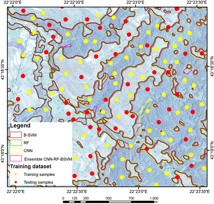
FIGURE 4. Results of vegetation classification.

As shown in Figure 5, the classification results produce roughly identical vegetation contours, especially in locations where the vegetation boundary is well separated in the images in comparison to other content. Smaller, but very significant differences are observed in the parts of the test area where the boundaries of vegetation are not clearly visible on the combination of satellite and aerial images. These minor deviations mostly affected the accuracy of the applied classification methods.

FIGURE 5

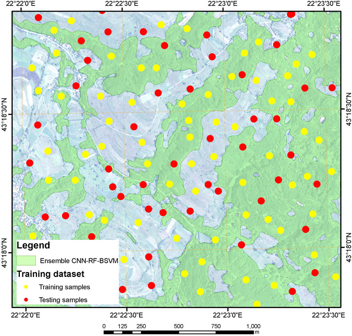
FIGURE 5. Proposed ensemble classification method with collected test samples.

For machine and deep learning classification accuracy testing, the confusion (error) matrix is widely utilized. A confusion matrix is a basic cross-tabulation of the predicted class label against the reference data for a sample of cases at certain locations, and it serves as a foundation for defining classification accuracy and characterizing errors. Many measures of classification accuracy can be derived from a confusion matrix: kappa coefficient, overall, user’s and producer’s accuracy. A confusions matrix are presented in the following tables: for biased Support vector machine classification in Table 3, for Random forest classification in Table 4, for Convolutional Neural Networks in Table 5, and finally for ensemble BSVM-RF-CNN in Table 6.

TABLE 3

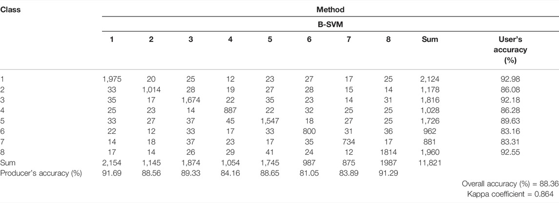
TABLE 3. Confusion (error) matrix for biased support vector machine (B-SVM) classification.

TABLE 4

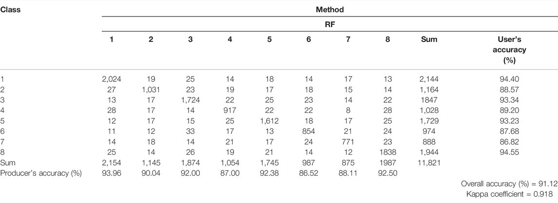
TABLE 4. Confusion (error) matrix for random forest (RF) classification.

TABLE 5

TABLE 5. Confusion (error) matrix for convolution neural network (CNN) classification.

TABLE 6

TABLE 6. Confusion (error) matrix for ensemble BSVM-RF-CNN classification.

All four approaches achieved high overall accuracies. In other circumstances, however, the suggested ensemble CNN-RF-BSVM approach outperformed the others. As shown in Table 3, reducing the number of satellite bands by deleting the less relevant ones does not result in a significant drop in classification accuracy. In the case of B-SVM, there is a significant increase in classification accuracy. This could be related to the requirement to simplify the vector space in order to build hyper-planes.

The values of the Kappa coefficients for vegetation classification from satellite pictures range from 0.864 for Biased Support vector machine classification to 0.923 for ensemble CNN-RF-BSVM classification (Tables 3–6).

In terms of the classification method utilized, it’s clear that combining machine learning with deep learning techniques for digital satellite and aerial image classification provides the potential for vegetation mapping and analyzing environmental changes. The use of a suitable machine learning or deep learning technique aids in the selection of an appropriate classification threshold as well as analysis bands. This reduces the need for trial and error procedures, which are frequently utilized when classifying data with a high degree of dimensionality.

5 Discussion

According to the achieved results, the biased Support vector machine has the lowest accuracy in relation to other techniques used. Before the classification stage, biased SVM and Random Forest algorithms usually include a feature generation and selection step. We discovered that the proposed criterion worked well for optimizing biased SVMs and outperformed an alternate optimization criterion in studying biased SVM for vegetation mapping. We also discovered that cross-validation performed at the crown level worked well (i.e., by splitting crowns rather than pixels into the cross-validation groups).

One of the B-SVM model’s biggest advantages is its non-linear categorization. A parametric model might thus have different intercepts and coefficient values for each class of discrete covariates. Furthermore, the B-SVM model is resistant to overfitting and is not overly impacted by noisy data. The B-SVM model benefits from complicated, non-linear interactions and is noise-resistant. The B-SVM method’s major flaw, on the other hand, is that it requires identifying the optimal model after testing multiple kernel combinations and model parameters. Meanwhile, because the results are part of a complicated black box model, they are extremely difficult to understand (Chan and King; Hartono et al., 2018).

Furthermore, for balanced data, the difficulty with biased SVM based on structural risk reduction in classification is that the classification weight will be biased towards the majority class, causing the classification hyperplane to be close to the minority class, making minority samples easy to misclassify (Chan and King; Hartono et al., 2018). Reducing the number of features also reduces overfitting concerns in remote sensing image classification, where high-dimensional data is available but ground truth data is scarce.

Random Forests are gradually becoming one of the most popular machine learning algorithms due to their power, diversity, and ease of use. The capacity to run on big datasets with a large number of predictors and its ability to handle thousands of input variables without variable deletion may explain why the RF performed better than the B-SVM and deep learning CNN models in this study (Cutler et al., 2007; Peters et al., 2007; Biau, 2012; Amini et al., 2018). The Random Forest model employs regression trees to estimate the dependent variable’s average as the final prediction, resulting in an internally unbiased calculation of the classification error. In comparison to other machine learning algorithms, the RF algorithm has significant advantages. Firstly, the RF technique can cope with noisy or missing data as well as categorical or continuous features; second, it does not require assumptions about the distribution of explanatory variables; and third, it can manage interactions and non-linearities between efficient components (Linardatos et al., 2020). These are significant advantages that reduce the production of outliers, especially when working with terrain variables that have a high frequency of missing data (Amini et al., 2018).

The Random Forests approach works by creating multiple classification trees throughout the training period, taking advantage of the considerable variation between individual trees. Furthermore, by randomly modifying the predictive variable sets and resampling the data with replacement over the many tree stages of induction, the Random Forests approach increases variation amongst the classification trees. Because the average results of all trees are the result of the model generation process, cross validation is not required for this method (Oliveira et al., 2012; Amini et al., 2018; Gigović et al., 2019a). The major flaw of the RF model, on the other hand, is that, unlike a decision tree, it is difficult to interpret. Furthermore, the proper use of the RF model may necessitate some effort to fine-tune the model for the data.

Convolutional neural networks can improve the likelihood of successful classifications if big enough data sets (hundreds to thousands of measurements, depending on the complexity of the topic under study) are available to describe the problem. The results show that CNN achieved high precision in the vast majority of the cases in which it was utilized, outperforming other common image-processing approaches (Kussul et al., 2017). Their key is their capacity to efficiently mimic exceedingly complicated problems and the fact that no prior experiments are required. It’s important to remember that visual classification and field research are only useful for obtaining reference data if the target species or type of vegetation can be easily identified in the imagery. This will be determined not only by the image quality (e.g., spatial resolution), but also by the uniqueness of the vegetation of interest’s morphological characteristics. In any event, CNN-based vegetation species identification is only useful if these morphological features are present in the plant canopy.

Because different machine and deep learning algorithms may not be capable of producing the best results on their own, integrating them will maximize the model’s potential and increase accuracy. It has been demonstrated that using an ensemble learning methodology to predict and classify a combination of satellite and aerial images produces better results than using a single classifier.

6 Conclusion

The performance of ensemble approaches for vegetation classification, which consists of three ML and DL algorithms, was investigated in this article. Two of these methods rely on machine learning, while the third is a deep learning approach. We use Bayesian averaging and efficient feature selection to create an ensemble model that addresses these difficulties and mitigates their effects on defect classification performance. The ensemble approach that utilized the RGB and NIR wavelengths worked reasonably well in tests. The results showed that the suggested ensemble model outperformed the DL and ML models in terms of overall accuracy by up to 7%, which was validated by the Wilcoxon signed-rank test. Overall accuracy (OA) analysis revealed that the suggested ensemble technique CNN-RF-BSVM greatly enhanced classification accuracy (by 4%).

Even though the proposed ensemble method can detect vegetation with a reasonable level of accuracy, one future research direction would be to use augmentation techniques with deep learning methods to diversify the training data so that more robust responses can be obtained when the test data characteristics differ significantly from the training data.

According to the results of the studies, the use of a combination of low spatial resolution satellite images and high spatial resolution aerial photogrammetry imagery for vegetation categorization mapping is practical, even though there is still room for improvement. Advanced radiometric image calibration techniques will be developed in the future to increase the quality of the images. Experimenting with better spectral resolution multispectral satellite images in combination with aerial photogrammetry images, which are becoming more cost-effective and possible, is also advised.

Data Availability Statement

The raw data supporting the conclusion of this article will be made available by the authors, without undue reservation.

Author Contributions

SD, MS DD, and SB prepared the data layers, figures, and tables; SD and MS performed the experiments and analyses. JJ and AD supervised the research, finished the first draft of the manuscript, edited and reviewed the manuscript, and contributed to the model construction and verification.

Funding

This work supported research project 1.1.107/2018 “Possibilities of automatic extraction of vegetation data by a combination of satellite and aerial photogrammetric images” by the Ministry of Defense of the Republic of Serbia and research project 1.21/2021 “Model for using MGI digital topographic maps in field conditions with portable devices” by the Ministry of Defense of the Republic of Serbia.

Conflict of Interest

The authors declare that the research was conducted in the absence of any commercial or financial relationships that could be construed as a potential conflict of interest.

Publisher’s Note

All claims expressed in this article are solely those of the authors and do not necessarily represent those of their affiliated organizations, or those of the publisher, the editors and the reviewers. Any product that may be evaluated in this article, or claim that may be made by its manufacturer, is not guaranteed or endorsed by the publisher.

References

Abdi, A. M. (2020). Land Cover and Land Use Classification Performance of Machine Learning Algorithms in a Boreal Landscape Using Sentinel-2 Data. GIScience Remote Sens. 57, 1–20. doi:10.1080/15481603.2019.1650447

CrossRef Full Text | Google Scholar

Adam, E., Mutanga, O., Abdel-Rahman, E. M., and Ismail, R. (2014). Estimating Standing Biomass in Papyrus (Cyperus Papyrus L.) Swamp: Exploratory of In Situ Hyperspectral Indices and Random Forest Regression. Int. J. Remote Sens. 35 (2), 693–714. doi:10.1080/01431161.2013.870676

CrossRef Full Text | Google Scholar

Amarsaikhan, D., and Douglas, T. (2004). Data Fusion and Multisource Image Classification. Int. J. Remote Sens. 25, 3529–3539. doi:10.1080/0143116031000115111

CrossRef Full Text | Google Scholar

Amini, S., Homayouni, S., Safari, A., and Darvishsefat, A. A. (2018). Object-based Classification of Hyperspectral Data Using Random Forest Algorithm. Geo-Spatial Inf. Sci. 21, 127–138. doi:10.1080/10095020.2017.1399674

CrossRef Full Text | Google Scholar

Ayhan, B., Kwan, C., Budavari, B., Kwan, L., Lu, Y., Perez, D., et al. (2020). Vegetation Detection Using Deep Learning and Conventional Methods. Remote Sens. 202012, 2502. doi:10.3390/RS12152502

CrossRef Full Text | Google Scholar

Bakrač, S., Drobnjak, S., Stanković, S., Vučićević, A., and Stamenković, N. (2018). “Preparation of Photogrammetric Archive Documentation for Scientific and Other Research,” in Sinteza 2018 - International Scientific Conference on Information Technology and Data Related Research. Belgrade, Serbia: Singidunum University. doi:10.15308/sinteza-2018-17-22

CrossRef Full Text | Google Scholar

Biau, G. (2012). Analysis of a Random Forests Model. J. Mach. Learn. Res. 13, 1063–1095.

Google Scholar

Breiman, L. (1996). Bagging Predictors. Mach. Learn 24, 123–140. doi:10.1007/BF00058655

CrossRef Full Text | Google Scholar

Breiman, L., and Cutler, A. (2007). Random Forests — Classification Description: Random Forests. http://stat-www.berkeley.edu/users/breiman/RandomForests/cc_home.htm

Google Scholar

Breiman, L. (2001). Random Forests. Mach. Learn. 45, 5–32. doi:10.1023/A:1010933404324

CrossRef Full Text | Google Scholar

Burai, P., Deák, B., Valkó, O., and Tomor, T. (2015). Classification of Herbaceous Vegetation Using Airborne Hyperspectral Imagery. Remote Sens. 7 (2), 2046–2066. doi:10.3390/rs70202046

CrossRef Full Text | Google Scholar

Chan, C.-H., and King, I. (2009). “Using Biased Support Vector Machine to Improve Retrieval Result in Image Retrieval with Self-Organizing Map,” in International Conference on Neural Information Processing. (Berlin, HDB: Springer), 714–719.

Google Scholar

Chan, J. C.-W., and Paelinckx, D. (2008). Evaluation of Random Forest and Adaboost Tree-Based Ensemble Classification and Spectral Band Selection for Ecotope Mapping Using Airborne Hyperspectral Imagery. Remote Sens. Environ. 112 (6), 2999–3011. doi:10.1016/J.RSE.2008.02.011

CrossRef Full Text | Google Scholar

Cutler, D. R., Edwards, T. C., Beard, K. H., Cutler, A., Hess, K. T., Gibson, J., et al. (2007). Random Forests for Classification in Ecology. Ecology 88, 2783–2792. doi:10.1890/07-0539.1

PubMed Abstract | CrossRef Full Text | Google Scholar

Dietterich, T. G. (2000). “Ensemble Methods in Machine Learning,” in International Workshop on Multiple Classifier Systems (Cagliari, Italy: Springer), 1–15. doi:10.1007/3-540-45014-9_1

CrossRef Full Text | Google Scholar

Dixit, A. (2019). Ensemble Classifier Based Multiclass Vegetation Classification System. ICTACT Journal on Image and Video Processing 10, 2076–2082. doi:10.21917/ijivp.2019.0295

CrossRef Full Text | Google Scholar

Doktor, D., Lausch, A., Spengler, D., and Thurner, M. (2014). Extraction of Plant Physiological Status from Hyperspectral Signatures Using Machine Learning Methods. Remote Sens. 6 (12), 12247–12274. doi:10.3390/rs61212247

CrossRef Full Text | Google Scholar

Drobnjak, S., Ćirović, G., Sekulović, D., and Regodić, M. (2013). Object-oriented Classification of Multispectral Landsat 7 Satellite Images. Metal. Int. 18, 206 Available att: http://www.scopus.com/inward/record.url?eid=2-s2.0-84874251767&partnerID=MN8TOARS.

Google Scholar

Drobnjak, S., Marković, V., Kričković, Z., and Vučičević, A. (2018). Vegetation Extraction from Satellite and Aerial Photogrammetric Images Using Machine Learning Algorithms” in 8th International Scientific Conference on Defensive Technologies, Serbia, October 11–12, 2018. Belgrade: MTI

Google Scholar

Emily, J. A., and Sudha, N. (2022). Case Studies: Deep Learning in Remote Sensing. Fundam. Methods Mach. Deep Learn., 425–437. doi:10.1002/9781119821908.CH18

CrossRef Full Text | Google Scholar

Engler, R., Waser, L. T., Zimmermann, N. E., Schaub, M., Berdos, S., Ginzler, C., et al. (2013). Combining Ensemble Modeling and Remote Sensing for Mapping Individual Tree Species at High Spatial Resolution. For. Ecol. Manag. 310, 64–73. doi:10.1016/J.FORECO.2013.07.059

CrossRef Full Text | Google Scholar

Fei, S., Li, L., Han, Z., Chen, Z., and Xiao, Y. (2022). A Novel Ensemble Method for Predicting Wheat Yield Using Feature Selection-Based Deep Learning and Hyperspectral Vegetation Indices. Res. Sq.. doi:10.21203/rs.3.rs-1392054/v1

CrossRef Full Text | Google Scholar

Fernández-Manso, A., Fernández-Manso, O., and Quintano, C. (2016). SENTINEL-2A Red-Edge Spectral Indices Suitability for Discriminating Burn Severity. Int. J. Appl. Earth Observation Geoinformation 50, 170–175. doi:10.1016/J.JAG.2016.03.005

CrossRef Full Text | Google Scholar

Foody, G. M., and Mathur, A. (2004). A Relative Evaluation of Multiclass Image Classification by Support Vector Machines. IEEE Trans. Geosci. Remote Sens. 42, 1335–1343. doi:10.1109/tgrs.2004.827257

CrossRef Full Text | Google Scholar

Gašparović, M., and Dobrinić, D. (2020). Comparative Assessment of Machine Learning Methods for Urban Vegetation Mapping Using Multitemporal Sentinel-1 Imagery. Remote Sens. 202012, 1952. doi:10.3390/RS12121952

CrossRef Full Text | Google Scholar

Ghimire, B., Rogan, J., and Miller, J. (2010). Contextual Land-Cover Classification: Incorporating Spatial Dependence in Land-Cover Classification Models Using Random Forests and the Getis Statistic. Remote Sens. Lett. 1 (1), 45–54. doi:10.1080/01431160903252327

CrossRef Full Text | Google Scholar

Ghosh, A., Fassnacht, F. E., Joshi, P. K., and Koch, B. (2014). A Framework for Mapping Tree Species Combining Hyperspectral and LiDAR Data: Role of Selected Classifiers and Sensor across Three Spatial Scales. Int. J. Appl. Earth Observation Geoinformation 26, 49–63. doi:10.1016/j.jag.2013.05.017

CrossRef Full Text | Google Scholar

Ghosh, H., and Prajneshu, M. A. (2011). Bootstrap Study of Parameter Estimates for Nonlinear Richards Growth Model through Genetic Algorithm. J. Appl. Statistics 38 (3), 491–500. doi:10.1080/02664760903521401

CrossRef Full Text | Google Scholar

Gigović, L., Pourghasemi, H. R., Drobnjak, S., Bai, S., Gigović, L., Pourghasemi, H. R., et al. (2019b). Testing a New Ensemble Model Based on SVM and Random Forest in Forest Fire Susceptibility Assessment and its Mapping in Serbia's Tara National Park. Forests 10, 408. doi:10.3390/F10050408

CrossRef Full Text | Google Scholar

Gigović, L., Pourghasemi, H. R., Drobnjak, S., and Bai, S. (2019a). Testing a New Ensemble Model Based on SVM and Random Forest in Forest Fire Susceptibility Assessment and its Mapping in Serbia's Tara National Park. Forests 10, 408. doi:10.3390/F10050408

CrossRef Full Text | Google Scholar

Hartono, H., Sitompul, O. S., Tulus, T., and Nababan, E. B. (2018). Biased Support Vector Machine and Weighted-SMOTE in Handling Class Imbalance Problem. Int. J. Adv. Intell. Inf. 4, 21–27. doi:10.26555/IJAIN.V4I1.146

CrossRef Full Text | Google Scholar

Kattenborn, T., Leitloff, J., Schiefer, F., and Hinz, S. (2021). Review on Convolutional Neural Networks (CNN) in Vegetation Remote Sensing. ISPRS J. Photogrammetry Remote Sens. 173, 24–49. doi:10.1016/J.ISPRSJPRS.2020.12.010

CrossRef Full Text | Google Scholar

Kavzoglu, T., Colkesen, I., and Yomralioglu, T. (2015). Object-based Classification with Rotation Forest Ensemble Learning Algorithm Using Very-High-Resolution WorldView-2 Image. Remote Sensing Letters 6, 834–843.

CrossRef Full Text | Google Scholar

Kussul, N., Lavreniuk, M., Skakun, S., and Shelestov, A. (2017). Deep Learning Classification of Land Cover and Crop Types Using Remote Sensing Data. IEEE Geosci. Remote Sens. Lett. 14, 778–782. doi:10.1109/LGRS.2017.2681128

CrossRef Full Text | Google Scholar

Landis, J. R., and Koch, G. G. (1977). An Application of Hierarchical Kappa-type Statistics in the Assessment of Majority Agreement Among Multiple Observers. Biometrics 33, 363. doi:10.2307/2529786

PubMed Abstract | CrossRef Full Text | Google Scholar

Li, Z., Hu, L., Tang, Z., and Zhao, C. (2021). Predicting HIV-1 Protease Cleavage Sites with Positive-Unlabeled Learning. Front. Genet. 12, 456. doi:10.3389/FGENE.2021.658078/BIBTEX

CrossRef Full Text | Google Scholar

Liaw, A., and Wiener, M. (2002). Classification and Regression by randomForest. R. News 2 (3), 18

Google Scholar

Linardatos, P., Papastefanopoulos, V., and Kotsiantis, S. (2020). Explainable Ai: A Review of Machine Learning Interpretability Methods. Entropy 23 (1), 18. doi:10.3390/e23010018

CrossRef Full Text | Google Scholar

Mallinis, G., Mitsopoulos, I., and Chrysafi, I. (2018). Evaluating and Comparing Sentinel 2A and Landsat-8 Operational Land Imager (OLI) Spectral Indices for Estimating Fire Severity in a Mediterranean Pine Ecosystem of Greece. GIsci. Remote. Sens. 55, 1–18. doi:10.1080/15481603.2017.1354803

CrossRef Full Text | Google Scholar

Meng, X., Shang, N., Zhang, X., Li, C., Zhao, K., Qiu, X., et al. (2017). Photogrammetric UAV Mapping of Terrain under Dense Coastal Vegetation: An Object-Oriented Classification Ensemble Algorithm for Classification and Terrain Correction. Remote Sens. 9, 1187. doi:10.3390/RS9111187

CrossRef Full Text | Google Scholar

Montgomery, J. M., Hollenbach, F. M., and Ward, M. D. (2012). Improving Predictions Using Ensemble Bayesian Model Averaging. Polit. Anal. 20, 271–291. doi:10.1093/PAN/MPS002

CrossRef Full Text | Google Scholar

Neto, U. M. B., and Dougherty, E. R. (2015). Error Estimation for Pattern Recognition. Hoboken, NY, United States: John Wiley & Sons.

Google Scholar

Nijhawan, R., Sharma, H., Sahni, H., and Batra, A. (2017). “A Deep Learning Hybrid CNN Framework Approach for Vegetation Cover Mapping Using Deep Features,” in Proceedings - 13th International Conference on Signal-Image Technology and Internet-Based Systems, SITIS 2017 2018-January, Jaipur, India, December 4–7, 2017, 192. doi:10.1109/SITIS.2017.41

CrossRef Full Text | Google Scholar

Oliveira, S., Oehler, F., San-Miguel-Ayanz, J., Camia, A., and Pereira, J. M. C. (2012). Modeling Spatial Patterns of Fire Occurrence in Mediterranean Europe Using Multiple Regression and Random Forest. For. Ecol. Manag. 275, 117–129. doi:10.1016/j.foreco.2012.03.003

CrossRef Full Text | Google Scholar

Peters, J., Baets, B. D., Verhoest, N. E. C., Samson, R., Degroeve, S., Becker, P. D., et al. (2007). Random Forests as a Tool for Ecohydrological Distribution Modelling. Ecol. Model. 207, 304–318. doi:10.1016/j.ecolmodel.2007.05.011

CrossRef Full Text | Google Scholar

Raftery, A. E., Gneiting, T., Balabdaoui, F., and Polakowski, M. (2005). Using Bayesian Model Averaging to Calibrate Forecast Ensembles. Mon. Weather Rev. 133, 1155–1174. doi:10.1175/MWR2906.1

CrossRef Full Text | Google Scholar

Running, S. W., Loveland, T. R., Pierce, L. L., Nemani, R. R., and Hunt, E. R. (1995). A Remote Sensing Based Vegetation Classification Logic for Global Land Cover Analysis. Remote Sens. Environ. 51, 39–48. doi:10.1016/0034-4257(94)00063-S

CrossRef Full Text | Google Scholar

Shaheen, F., and Verma, B. (2016). “An Ensemble of Deep Learning Architectures for Automatic Feature Extraction,” in 2016 IEEE Symposium Series on Computational Intelligence, 1–5. (Athens, Greece: SSCI). doi:10.1109/SSCI.2016.7850047

CrossRef Full Text | Google Scholar

Sothe, C., de Almeida, C. M., Schimalski, M. B., Liesenberg, V., la Rosa, L. E. C., Castro, J. D. B., et al. (2020). A Comparison of Machine and Deep-Learning Algorithms Applied to Multisource Data for a Subtropical Forest Area Classification. Int. J. Remote. Sens. 41, 1943–1969. doi:10.1080/01431161.2019.1681600

CrossRef Full Text | Google Scholar

Vrugt, J. A., and Robinson, B. A. (2007). Treatment of Uncertainty Using Ensemble Methods: Comparison of Sequential Data Assimilation and Bayesian Model Averaging. Water Resour. Res. 43, 1411. doi:10.1029/2005WR004838

CrossRef Full Text | Google Scholar

Wang, H., Lv, G., Cai, Y., Zhang, X., Jiang, L., and Yang, X. (2021). Determining the Effects of Biotic and Abiotic Factors on the Ecosystem Multifunctionality in a Desert-Oasis Ecotone. Ecol. Indic. 128, 107830. doi:10.1016/J.ECOLIND.2021.107830

CrossRef Full Text | Google Scholar

Woolson, R. F. (2008). Wilcoxon Signed-Rank Test, 1–3. Wiley Encyclopedia of Clinical Trialsdoi:10.1002/9780471462422.EOCT979 (Accessed September 18, 2008)

CrossRef Full Text | Google Scholar

Xie, Y., Sha, Z., and Yu, M. (2008). Remote Sensing Imagery in Vegetation Mapping: a Review. J. Plant Ecol. 1, 9–23. doi:10.1093/JPE/RTM005

CrossRef Full Text | Google Scholar

Yu, Q., Gong, P., Clinton, N., Biging, G., Kelly, M., and Schirokauer, D. (2006). Object-based Detailed Vegetation Classification with Airborne High Spatial Resolution Remote Sensing Imagery. Photogramm. Eng. remote Sens. 72, 799–811. doi:10.14358/PERS.72.7.799

CrossRef Full Text | Google Scholar

Zhang, X., Han, L., Han, L., and Zhu, L. (2020). How Well Do Deep Learning-Based Methods for Land Cover Classification and Object Detection Perform on High Resolution Remote Sensing Imagery? Remote Sens. 12, 417. doi:10.3390/RS12030417

CrossRef Full Text | Google Scholar