Analysis of Ambient Air PM10-Bound Pollutants Surrounding an Industrial Site and Their Prediction Using Artificial Neural Network

The 2030 Agenda dictated the Sustainable Development Goals. It states the waste reduction needs through their reuse, i.e., considering them as secondary raw materials (Objective 12.5). Bottom ashes from municipal or industrial incinerators can be reused as partial cement replacement in concrete after preventive physical processes such as ferrous metals removal (magnetic separation) and nonferrous metals removal (Eddy current separation). Net of the principal pollutant containment systems, diffusive emissions of fine particles from these processes, coupled with several screening steps and a final long-time open-air residues stabilization, could impact the surrounding environment due to the chemical composition of the particulate matter itself (inorganic and organic pollutants). Moreover, the particulate may also arise from transporting the raw bottom ashes to the pre-treatment plant (point source). The present work aims to predict the concentration of the PM10-bound organic contaminants that are usually sampled weekly (PCDD/Fs, PCBs, PAHs) from the concentration of the daily analyzed inorganic pollutants in the surrounding area of an municipal solid waste slag treatment plant, using Artificial Neural Networks (ANNs) as a forecasting tool. Moreover, ANNs have also been used as a clustering tool to evaluate the plant’s environmental impact on the surrounding area with respect to other additional emission sources.

Introduction

A combustion process creates heat that is recycled and reused or converted to electrical energy. The fate of the residues (fly and bottom ashes) depends on their characteristics. The thermal treatment plants’ residues from power production and municipal or industrial wastes show pozzolanic properties. They can be used as secondary raw materials for cement and building material production. (Giergiczny 1991; Kumar and Singh 2021; Mafalda Matos and Sousa-Coutinho 2022). This statement agrees with the request of the 2030 Agenda to protect the planet from degradation by minimizing waste generation through prevention, reduction, recycling, and reuse, as mentioned in its objective 12.5 (United Nations 2015). After incineration, bottom ashes are mainly composed of slag, synthetic ceramics, minerals, ferrous and nonferrous metals, unburned organic matter, glass, porcelain, and soluble salts such as hydroxides and chlorides. They are preliminarily screened to remove bigger particles, after which they are subjected to physical treatments such as magnetic separation to extract ferrous materials and Eddy current separation to remove nonferrous metal constituents. They undergo a final long-time open-air stabilization. This can last up to 6–9 months, and it is used to weather/oxidize the components mainly by the action of O₂, CO₂, and water. The pH of the bottom ashes bulk will decrease, allowing the constituents’ modification from hydroxides to sulfate than to carbonates, decreasing their leachability and dramatically contributing to the heavy metals leaching reduction (Chimenos et al., 2003). Finally, bottom ashes are sieved with different meshes to create aggregates showing several physical and mechanical characteristics such as density, compressive strength, and flexural strength, making them suitable for various uses in construction either directly or as an aggregate in other materials (Saffarzadeh et al., 2011; Spreadbury et al., 2021; Y.; Kim and Lee 2002; Youcai 2017; Astrup et al., 2016; Koksal et al., 2021). Prior to any other considered use, their environmental impact must be proven. It means sampling, analysis, and data processing. The focus is on the content of metals and persistent organic pollutants (POPs) due to the toxic aspects (Kim et al., 2004; Wei et al., 2021). The analysis of POPs (i.e., PCDD/Fs, PCBs, and PAHs) requires multiple days of sampling (due to the low concentrations in air, an enrichment of the sample is necessary to have an amount greater than the instrumental limit of quantification) and the laboratory analysis (extraction, analysis and data processing) requires at least 2 days. Usually, airborne metals are collected daily on filters and then determined by Inductively Coupled Plasma–Optical Emission Spectrometer (ICP-OES), Atomic Emission Spectrometer (AES), Mass Spectrometer (MS), and X-ray fluorescence (XRF) (Suvarapu and Baek, 2017).

Artificial neural networks (ANNs) are computational methodologies that perform multifactorial analyses. Inspired by biological neuron processes, the concept was introduced in 1943 by McCulloch and Pitts, simulating how the human brain processes information through the nerve cells, or neurons, connected to each other in a complex network within a computational model (McCulloch and Pitts, 1943). ANNs can model complicated and non-linear relationships. Moreover, from a modeling perspective, it works as a black box (Mjalli et al., 2007): it can approximate any function, studying its structure, but it cannot give any insights about the structure of the function being approximated. Therefore, ANNs can process the available data (input) and produce a prediction of the target value (output), identifying and learning the effects of an unknown complex cause-effect relationship between input and output through a training process. A neural network can approximate a wide range of statistical models without hypothesizing in advance any relationships between the dependent and independent variables. Instead, the form of the relationships is determined during the learning process. If a linear relationship between the dependent and independent variables is appropriate, the neural network results should closely approximate those of the linear regression model. If a non-linear relationship is more appropriate, the neural network will automatically match the “correct” model structure. The neuron (node) is the basic processing unit in neural networks. Neural networks impose minimal demands on model structure and assumptions. Still, it is necessary to choose the general network architecture correctly, consisting of multiple layers of nodes in a directed graph. Each layer is fully connected to the next one.

ANNs are a useful statistical tool for solving classifications, clustering, regression, pattern recognition, dimension reduction, structured prediction, machine translation, anomaly detection, decision making, visualization, and computer vision problems. They are often used as alternative forecasting methods in many fields, such as marketing, meteorology, and finance, where a significant amount of data is challenging to manage. In environmental sciences, they have been recently used in the prediction of sorption/desorption of chemicals from soil (Silva et al., 2019), delineation of soil contaminant plumes (Tao et al., 2019), risk assessment, and spatial modeling of heavy metals (Abbaszadeh et al., 2020), soil infiltration in furrow irrigation (Nazli et al., 2019), determination of principal components affecting soil infiltration (Alipour et al., 2021), forecasting the change in organic agricultural output (Doan 2021), investigating in PAHs bioremediation (Bao et al., 2019) and investigating the atmospheric sciences (Gardner and Dorling 1998). Many researches were performed using ANNs for air pollutant time series modeling and air pollutant concentrations forecasting, describing this method as good training, validation, and testing techniques and discussing measurements of performance and reliability (Prachi and Matta, 2011). An ANNs model has also been used to forecast short and middle long-term concentration levels of well-known air pollutants (Viotti et al., 2002). The method has shown outstanding performances for the short forecasts. For the medium and long-term forecasts, the results are better than the usual deterministic models in terms of mean square error (MSE), introducing hypotheses about the values of the meteorological and traffic parameters. Other studies have compared the predictive ability of the ANN models (non-linear method) for forecasting concentrations of air pollutants with the Multi-Linear Regression (MLR), proving that MLR is better than ANNs except in a few cases (Cakir and Moro 2020).

A multilayer perceptron (MLP) is a class feedforward artificial neural network. It consists of three or more layers (an input and an output layer with one or more hidden layers) of nonlinearly activating nodes: it is a function of predictors (also called inputs or independent variables) that minimize the prediction error of target variables (also called outputs). An example of MLP’s architecture is shown in Supplementary Material S1.

The MLP model is an example of a feedforward neural network, referring to a fully connected network with three or more layers (an input and an output layer with one or several hidden layers) of nonlinearly activating nodes. The connections are unidirectional, and there are no cycles or loops in the network; thus, each neuron is linked only to neurons in the next layer. Each layer is connected to the adjacent neurons through an activation function, and all connections have their weights.

The MLP’s Learning Process Occurs in the Following Consecutive Phases

a) Training (or calibration) phase: the original input set is divided into three subsets: training set, test set, and holdout set (Riad et al., 2004). The MLP reads the input and output variables of the training set and optimizes the prediction error of the output.

b) Testing (or verification) phase: the model accuracy is estimated by error indicators such as the Coefficient of determination (R²) and the Root Mean Square Error (RMSE) of prediction calculated for the holdout set. The minimum RMSE and the maximum R² are often used to select the “better” neural network (Afan et al., 2015). RMSE is calculated in both the training and test set. Comparing both values, if they are of the same order of magnitude, the neural network provides reliable predictions (Chaloulakou et al., 2003).

As previously stated, the analysis of POPs is time- and cost-consuming. In this study, an MLP model has been used to predict the concentration of PM10-bound organic micropollutants (PCDD/Fs, dl-PCBs, and PAHs) from the concentration of daily airborne metals in an area where a municipal solid waste (MSW) bottom slag recovery plant is present, also considering whether it is possible to apply the neural networks for identifying the different emission sources. This work aims to underline that ANNs can be a helpful tool for predicting the concentrations of persistent pollutants and as a support tool for the plant manager to reduce the fallout of its emissions on the ground.

Materials and Methods

Sampling Area and Strategy

This section provides information related to ambient air sample data collection. The industrial plant, focus of this work, bottom slag recovery plant. It is a mechanical slag treatment in an industrial-covered shed. There is an aspiration system for collecting and treating dust emissions generated by processing incoming waste and bag filters for air filtration. The plant is in a mainly periurban area, where other productive settlements are located (concrete production, semi-finished food products, carpentry, welding). Ambient air samples were collected at three sites, named A, B, and C, selected based on the position of the industrial plant (distance, wind direction). In detail, site A can be considered representative of the maximum fallout of the plant, as it is located within the perimeter of the plant itself; site B is located 4 km West of the plant, in a suburban site, on a moderately high-traffic road; site C is located 3 km East of the plant, in an urban park.

Ambient air samples were collected in two experimental campaigns in summer and winter, lasting 3 weeks each. Air samples were collected using a high-volume sampler (Echo PUF high volume sampler, TCR Tecora, Milan, Italy), equipped with a quartz fiber filter (QFF) and a polyurethane foam (PUF), allowing simultaneous sampling of particulates and gases at a flow rate of 200 L/min for organic micropollutants, and with a SkyPost PM10 sampler for the collection of particulate matter on which the subsequent analysis of metals was carried out. The organic micropollutants were collected weekly (18 samples), whereas the particulate matter was collected daily.

Chemical Analysis

Once collected, the samples were sent to the laboratory for analysis. Each QFF + PUF sample was spiked with standard solutions (Wellington Lab, Canada) containing PCDD/Fs (EN-1948 ES) and dl-PCBs (WP-LCS) prior to the extraction process (36 h Soxhlet extraction with toluene). The extract was concentrated and divided into two fractions - one for PAHs and one for separating PCDD/Fs and PCBs. A subsequent clean-up followed (Mosca et al., 2010) prior to the instrumental GC/MS analysis. The analysis of metals was based on the extraction of each filter in an ultrasonic bath, extraction of the residue via acid digestion, and the subsequent ICP/MS analysis of both fractions, according to Canepari et al. (2006).

Statistical Analysis

In this work, preliminary correlation analysis has been performed, investigating the possible linearity of the relationships between the considered variables employing Pearson’s correlation matrix. If there is a linear dependence between organic, PM10, and inorganic variables, it could be assumed that the same emission source is present. Then, a Principal Component Analysis (PCA) is processed to increase the interpretability of the variable’s relationships. Finally, a Multilayer Perceptron algorithm has been carried out, considering PM10 and 27 metals as input variables and the organic contaminants (TCDD, ∑ PCDD/F, ∑ PCB, BaP, and ∑ PAHs as the output to be predicted. Daily data for PM10 and metals were aggregated on a weekly basis to carry out a consistent analysis.

All statistical applications were performed using the software package SPSS v. 27.

Results and Discussion

Preliminary Statistical Analysis

As mentioned above, a preliminary analysis for the study of linear dependence was performed. PM10, 27 metals (independent variables or input), and organic micropollutants (dependent variables or output) were analyzed from 18 air samples. Among micropollutants, 2.3,7,8-tetrachlorodibenzo-p-dioxin (TCDD) and benzo(a)pyrene (BaP) were considered, along with the sum of PAHs, PCDD/Fs, and dioxin-like PCBs, due to their toxicological aspect. Pearson’s correlation matrix with the significance level at p < 0.05 is shown in the Supplementary Material S1.

Correlation analysis shows the presence of multicollinearity: two or more of the predictors (or input variables) are moderately or highly correlated with one another. This occurs, for instance, for As and Co., whose Pearson’s correlation coefficient r², at a significance level of 0.05, is equal to 0.93, or for Fe and Cr, with r² equal to 0.97.

Some important relationships are also observed between predictors and dependent variables. For example, TCDD is negatively correlated with Mg, with r² equal to -0.65; ∑ PCB has a linear correlation with Cr and Fe (r² equal to 0,63 and 0.60, respectively); BaP and ∑ PAHs are positively correlated with Tl, with r² as 0.76 and 0.70 respectively, and negatively correlated with Ba (r² as -0.75 and -0.70, respectively), Mg (r² as -0.70 and -0.64, respectively), Ni (r² as -0.68 and -0.61, respectively) and V (r² as -0.73 and -0.68, respectively). At the same time, ∑ PCDD/Fs do not correlate with any metal. The presence of linear relationships allows us to hypothesize for organic and inorganic contaminants with the same emission source and to perform forecasts through traditional methods, such as the Multi Linear Regression. The next step was the application of the Principal Component Analysis (PCA) to find out if there were any latent relationships between the variables ∑ PCDD/Fs and metals. In other words, PCA was used as data clustering to identify if and–eventually - which metal influences the presence of PCDD/Fs (and the other organic pollutants) to be referred to as the same contamination source.

The PCA’s process computes six principal components by varimax orthogonal rotation criterium, as described in Table 1.

TABLE 1

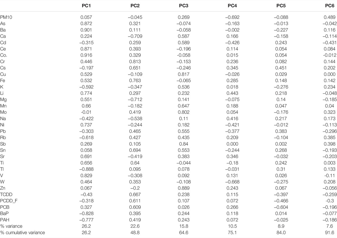
TABLE 1. Principal Component Analysis (PCA).Rotated component matrix and variance explained.

The first six PCs accounted for 91.6% of the total variation in the dataset: a six-dimensional space is supposed to be an excellent approximation to the original scatterplot of 33 variables, but it is not graphically representable. Furthermore, the first three PCs accounted only for 64.6% of the cumulative variance, and any cluster within the component plot is difficult to define (Figure 1).

FIGURE 1

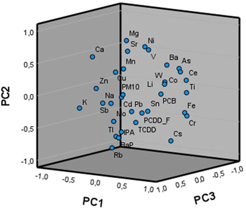
FIGURE 1. The three-dimensional component plot in rotated space.

It has thus been shown that PCA cannot clearly identify the sources of pollution, justifying the concomitant emission of PM10 and some metals with organic contaminants. Therefore, it was decided to apply an additional statistical clustering method to study the potential aggregations between variables and to explain the simultaneous presence of the variables considered in the same site.

The idea behind it all was to investigate the cause/effect relationships between all pollutants, in the three sites, by predicting the concentration of each organic component (output) resulting from PM10 and metals (input) through the development of an MLP model. The MLP, being a non-parametric technique, has been preferred to any other predictive method because the net can provide reliable results without hypothesizing in advance any relationships between the dependent and independent variables.

Artificial Neural Networks Results

Generally, ANNs models are considered a fundamental tool for collecting information about an extensive data system, but they can process small datasets. Referring to five output variables and 28 input variables (PM10 and the 27 metals), two MLP models have been performed for each organic contaminant (TCDD, PCDD/F, PCB, BaP, and PAHs), first considering all the 18 samples collected at the three sampling points, called Zone T (Sites A, B, and C), and then considering only the 12 samples placed outside the treatment plant, called Zone E (Sites B and C).

Each net has an MLP architecture 28-nine to one, where “28” is referred to the input variables (PM10 and 27 metals), “9” refers to the hidden variables (in one hidden layer), and “1” is referred to the output variables (organic contaminants). MLP architecture is shown in Supplementary Material S1.

The training set was used to train the network and the test set to evaluate the prediction performance of the ten models. R² and RMSE of the training and test set values are displayed in Table 2.

TABLE 2

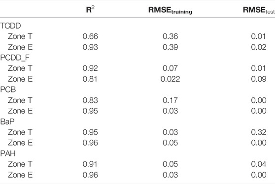
TABLE 2. ANNs performance evaluation.

All values of R² are over 0.80, except for TCDD in zone T (0.66). Furthermore, the RMSE values in the training and test set are all in the same order. Therefore, the MLP models in Zone T and E provide reliable predictions.

The results for Zone T and Zone E models do not differ significantly, except for the TCDD variable, as the network could not “read” any relationships between TCDD and metals in samples from Site A (treatment plant). ANN predictive capability is higher for external samples (Zone E) than for the total of the samples (Zone T = Zone E + treatment plant) except for the variable PCDD/Fs. Among the external samples, the Urban site (site B) is more distant from the plant and influenced by ordinary traffic and trucks that go back and forth from the plant. This peculiarity impacts PCDD/F values and seems to affect the predictive capacity of the network adversely. The source of dioxin emission at this site is unknown and will be further investigated. It is also noted that anomalous values are recorded at the same site in the case of PCB-126 (3.3′,4.4′,5-PentaCB) and PCB-169 (3.3′,4′,5.5′-HexaCB).

A T-test for two independent groups has been applied to confirm if the performance of the Zone T and Zone E models provides similar analytical results for the other variables (Johnson and Wickern, 2014). The outcome of this test is the acceptance or rejection of the null hypothesis (H₀) within a predefined confidence level, generally at 95%. The null hypothesis states that any differences or outlying results are purely due to random and not systematic errors. The alternative hypothesis (H₁) states precisely the opposite. Even though it is true, an erroneous rejection of H₀ constitutes a “type 1 error” or p-value. A smaller p-value means stronger evidence in favor of the alternative hypothesis. The most commonly used p-value is 0.05. To accept or reject H₀, the observed t-statistic text has to fall within the acceptance region (AR). The AR boundaries depend on the significance level of the test (the probability of erroneously rejecting the null hypothesis). Then they are calculated as a function of the p-value.

In this study, H₀ is the hypothesis that the predictive capability of both Zone T and Zone E models is the same for each output variable. T-test results are explained in the following Table 3.

TABLE 3

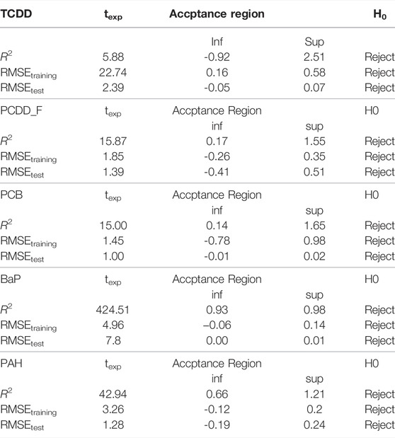
TABLE 3. T-test results.

For each organic pollutant, the test leads to the rejection of the null hypothesis: the predictive capability of the models is very different not only for TCDD but also for other variables despite the agreement between R² and RMSE values.

Conclusion

This study analyzed the concentration data of persistent organic micro-pollutants (PCDD/Fs, PCBs, and PAHs), PM10, and metals potentially emitted from an MSW residual treatment plant in ambient air. The traditional statistical approach could not clearly identify the sources of contaminants proving the same release of PM10, metals, and organic pollutants. ANN via MLP models was then applied to the dataset (concentration in three sampling sites), considering PM10 and metals as input and organic pollutants as output. As the first goal of this study, the contribution of the plant’s emissions to the surrounding air was evaluated by differentiating the data analysis of the sampling sites: “T zone,” including all three sites, and “E zone,” including only the two most distant sites from the plant, thus excluding the concentrations in the site of maximum relapse.

An assessment of the predictive capability of the models (R² and RMSE) in both areas (inside and outside the plant) identified that the emission sources of external and internal samples were different. Therefore, the network’s performance was higher for TCDD, PCB, BaP, and PAHs when only external samples were considered (even if the sample numbers are lower) since the model relationships were “contaminated” by the pollution sources within the treatment plant.

According to the R² values, the E model (external sites) for TCDD, PCB, BaP, and PAH provides more reliable predictions than the T Model (all sites) though with fewer samples, as if the stationary emission source due to the plant was “clouding” the relationships between the different pollutants. Conversely, in Zone E, the ANNs can better interpret the relationships. For PCDD/F, T Model is better than E Model: the relationships between the contaminants in the three sampling sites are more straightforward and allow the network to “learn” more.

Given the correspondence between the input and output data, it is possible to control the emission of micropollutants by monitoring the concentration of PM10 and metals (input). Furthermore, from an analytical point of view, it is easier and cheaper to obtain PM10 and metals data than POPs. This means that anomalous data of PM10 and/or metals (a daily event) and a higher concentration of POPs could be associated. In this case, it would be possible to promptly start the weekly sampling, thus reducing the costs of air quality analysis. Moreover, since pollutants are emitted from multiple sources, stationary and mobile, the application of ANN as a predictive tool can even support the plant manager (stationary source), acting on operative parameters (i.e., feeding, abatement systems, … ) to control polluting emissions. In this way, the contribution to the total concentration of organic micropollutants in ambient air in the surrounding area can be monitored and eventually minimized almost in real-time.

Data Availability Statement

The datasets presented in this article are not readily available because they are part of private ownership. Requests to access the datasets should be directed silvia.mosca@iia.cnr.it.

Author Contributions

Conceptualization: MB, AM, and SM; data curation, MC, EG, SM, MP, and GR; formal analysis: MB; investigation, MB; methodology: MB; project administration: AM and SM; resources, AM, EG, SM, and GR; supervision, MB, AM, and SM; validation, MB; visualization, MB and AM; writing—original draft, MB, A.M. and SM; writing—review and editing, MB, AM, and SM All authors have read and agreed to the published version of the manuscript.

Conflict of Interest

Authors MA and RG are employed by Chemical Research 2000 Srl.

The remaining authors declare that the research was conducted in the absence of any commercial or financial relationships that could be construed as a potential conflict of interest.

Publisher’s Note

All claims expressed in this article are solely those of the authors and do not necessarily represent those of their affiliated organizations, or those of the publisher, the editors and the reviewers. Any product that may be evaluated in this article, or claim that may be made by its manufacturer, is not guaranteed or endorsed by the publisher.

Acknowledgments

We want to thank Adriano Genovese for his careful revision of the text of the paper.

Supplementary Material

The Supplementary Material for this article can be found online at: https://www.frontiersin.org/articles/10.3389/fenvs.2022.893824/full#supplementary-material

References

Abbaszadeh, Maliheh, Mirzaei, Rouhollah, and Bakhtiari, Asra (2020). Risk Assessment and Spatial Modeling of Heavy Metals Contamination in Topsoil Around Venarj Manganese Mine by Artificial Neural Networks Method. J. Environ. Health Eng. 0 (0), 24–44. doi:10.29252/JEHE.0.24

CrossRef Full Text | Google Scholar

Afan, H. A., El-Shafie, A., Yaseen, Z. M., Hameed, M. M., Wan Mohtar, W. H. M., and Hussain, A. (2015). ANN Based Sediment Prediction Model Utilizing Different Input Scenarios. Water Resour. Manage 29 (4), 1231–1245. doi:10.1007/s11269-014-0870-1

CrossRef Full Text | Google Scholar

Alipour, Nazli, Nasseri, Abolfazl, Mohammdi Torkashvand, Ali, and Pazira, Ebrahim (2021). Detecting the Principal Components Affecting Soil Infiltration Using Artificial Neural Networks. Soil Environ. 40 (1), 9–16. doi:10.25252/SE/2021/112007

CrossRef Full Text | Google Scholar

Alipour, N., Nasseri, A., Ali, Mohammdi Torkashvand, and Ebrahim, Pazira (2019). Interpolation of Soil Infiltration in Furrow Irrigation: Comparison of Kriging, Inverse Distance Weighting, Multilayer Perceptron and Principal Component Analysis Methods. pjss 52 (1), 59–73. doi:10.17951/pjss/2019.52.1.5910.17951/pjss.2019.52.1.59

CrossRef Full Text | Google Scholar

Astrup, T., Muntoni, A., Polettini, A., Pomi, R., Van Gerven, T., and Van Zomeren, A. (2016). Treatment and Reuse of Incineration Bottom Ash. Environ. Mater. Waste Resour. Recovery Pollut. Prev. January, 607–645. doi:10.1016/B978-0-12-803837-6.00024-X

CrossRef Full Text | Google Scholar

Bao, H., Wang, J., Li, J., Zhang, H., and Wu, F. (2019). Effects of Corn Straw on Dissipation of Polycyclic Aromatic Hydrocarbons and Potential Application of Backpropagation Artificial Neural Network Prediction Model for PAHs Bioremediation. Ecotoxicol. Environ. Saf. 186 (December), 109745. doi:10.1016/J.ECOENV.2019.109745

PubMed Abstract | CrossRef Full Text | Google Scholar

Cakir, S., and Sita, M. (2020). Evaluating the Performance of ANN in Predicting the Concentrations of Ambient Air Pollutants in Nicosia. Atmos. Pollut. Res. 11 (12), 2327–2334. doi:10.1016/J.APR.2020.06.011

CrossRef Full Text | Google Scholar

Canepari, S., Cardarelli, E., Pietrodangelo, A., and Strincone, M. (2006). Determination of Metals, Metalloids and Non-volatile Ions in Airborne Particulate Matter by a New Two-step Sequential Leaching procedurePart B: Validation on Equivalent Real Samples. Talanta 69 (3), 588–595. doi:10.1016/J.TALANTA.2005.10.024

PubMed Abstract | CrossRef Full Text | Google Scholar

Chaloulakou, A., Saisana, M., and Spyrellis, N. (2003). Comparative Assessment of Neural Networks and Regression Models for Forecasting Summertime Ozone in Athens. Sci. Total Environ. 313 (1–3), 1–13. doi:10.1016/S0048-9697(03)00335-8

PubMed Abstract | CrossRef Full Text | Google Scholar

Chimenos, J. M., Fernández, A. I., Miralles, L., Segarra, M., and Espiell, F. (2003). Short-Term Natural Weathering of MSWI Bottom Ash as a Function of Particle Size. Waste Manag. 23 (10), 887–895. doi:10.1016/S0956-053X(03)00074-6

PubMed Abstract | CrossRef Full Text | Google Scholar

Doan, Huy Quang (2021). Forecasting the Change in Organic Agricultural Output in the Northern Midland and Mountainous Provinces of Vietnam Based on Artificial Neural Network Model. Int. J. Bus. 26 (4), 119–132.

Google Scholar

Gardner, M. W., and Dorling, S. R. (1998). Artificial Neural Networks (The Multilayer Perceptron)—A Review of Applications in the Atmospheric Sciences. Atmos. Environ. 32 (14–15), 2627–2636. doi:10.1016/S1352-2310(97)00447-0

CrossRef Full Text | Google Scholar

Giergiczny, Z. (1991). The Wastes from Power Plants as Substitute of Natural Raw Materials. Stud. Environ. Sci. 48, 619–620. doi:10.1016/S0166-1116(08)70454-0

CrossRef Full Text | Google Scholar

Johnson, R. A., and Wichern, D. W. (2014). Applied Multivariate Statistical Analysis. 6th Edn. Edinbugh: Pearson Educational Ltd.

Kim, K.-H., Seo, Y.-C., Nam, H., Joung, H.-T., You, J.-C., Kim, D.-J., et al. (2005). Characteristics of Major Dioxin/furan Congeners in Melted Slag of Ash from Municipal Solid Waste Incinerators. Microchem. J. 80, 171–181. doi:10.1016/j.microc.2004.07.022

CrossRef Full Text | Google Scholar

Kim, Y., and Lee, D. (2002). Solubility Enhancement of PCDD/F in the Presence of Dissolved Humic Matter. J. Hazard Mater 91 (1–3), 113–127. doi:10.1016/S0304-3894(01)00364-8

PubMed Abstract | CrossRef Full Text | Google Scholar

Koksal, F., Gencel, O., Sahin, Y., and Okur, O. (2021). Recycling Bottom Ash in Production of Eco-Friendly Interlocking Concrete Paving Blocks. J. Mater Cycles Waste Manag. 23, 985–1001. doi:10.1007/s10163-021-01186-8

CrossRef Full Text | Google Scholar

Kumar, S., and Singh, D. (2021). Municipal Solid Waste Incineration Bottom Ash: A Competent Raw Material with New Possibilities. Innov. Infrastruct. Solut. 6, 201. doi:10.1007/s41062-021-00567-0

CrossRef Full Text | Google Scholar

Mafalda Matos, A., and Sousa-Coutinho, J. (2022). Municipal Solid Waste Incineration Bottom Ash Recycling in Concrete: Preliminary Approach with Oporto Wastes. Constr. Build. Mater. 323 (March), 126548. doi:10.1016/J.CONBUILDMAT.2022.126548

CrossRef Full Text | Google Scholar

McCulloch, W. S., and Pitts, W. (1943). A Logical Calculus of the Ideas Immanent in Nervous Activity. Bull. Math. Biophysics 5, 115–133. doi:10.1007/bf02478259

CrossRef Full Text | Google Scholar

Mjalli, F. S., Al-Asheh, S., and Alfadala, H. E. (2007). Use of Artificial Neural Network Black-Box Modeling for the Prediction of Wastewater Treatment Plants Performance. J. Environ. Manag. 83 (3), 329–338. doi:10.1016/J.JENVMAN.2006.03.004

CrossRef Full Text | Google Scholar

Mosca, S., Torelli, G. N., Guerriero, E., Tramontana, G., Pomponio, S., Rossetti, G., et al. (2010). Evaluation of a Simultaneous Sampling Method of PAHs, PCDD/Fs and Dl-PCBs in Ambient Air. J. Environ. Monit. 12 (5), 1092–1099. doi:10.1039/b927004c

PubMed Abstract | CrossRef Full Text | Google Scholar

Prachi, Nishant Kumar, and Matta, Gagan (2011). Artificial Neural Network Applications in Air Quality Monitoring and Management. Int. J. Environ. Rehabilatation Conservation 2 (1), 1631–1638.

Google Scholar

Riad, S., Mania, J., Bouchaou, L., and Najjar, Y. (2004). Predicting Catchment Flow in a Semi-arid Region via an Artificial Neural Network Technique. Hydrol. Process. 18 (13), 2387–2393. doi:10.1002/hyp.1469

CrossRef Full Text | Google Scholar

Saffarzadeh, A., Shimaoka, T., Wei, Y., Gardner, K. H., and Musselman, C. N. (2011). Impacts of Natural Weathering on the Transformation/Neoformation Processes in Landfilled MSWI Bottom Ash: A Geoenvironmental Perspective. Waste Manag. 31 (12), 2440–2454. doi:10.1016/J.WASMAN.2011.07.017

PubMed Abstract | CrossRef Full Text | Google Scholar

Silva, T. S., de Freitas Souza, M., Maria da Silva Teófilo, T., Silva dos Santos, M., Formiga Porto, M. A., Martins Souza, C. M., et al. (2019). Use of Neural Networks to Estimate the Sorption and Desorption Coefficients of Herbicides: A Case Study of Diuron, Hexazinone, and Sulfometuron-Methyl in Brazil. Chemosphere 236 (December), 124333. doi:10.1016/J.CHEMOSPHERE.2019.07.064

PubMed Abstract | CrossRef Full Text | Google Scholar

Spreadbury, C. J., McVay, M., Laux, S. J., and Townsend, T. G. (2021). A Field-Scale Evaluation of Municipal Solid Waste Incineration Bottom Ash as a Road Base Material: Considerations for Reuse Practices. Resour. Conservation Recycl. 168 (May), 105264. doi:10.1016/J.RESCONREC.2020.105264

CrossRef Full Text | Google Scholar

Suvarapu, L. N., and Baek, S.-O. (2017). Determination of Heavy Metals in the Ambient Atmosphere. Toxicol. Ind. Health 33 (January), 79–96. doi:10.1177/0748233716654827

PubMed Abstract | CrossRef Full Text | Google Scholar

Tao, H., Liao, X., Zhao, D., Gong, X., and Cassidy, D. P. (2019). Delineation of Soil Contaminant Plumes at a Co-contaminated Site Using BP Neural Networks and Geostatistics. Geoderma 354 (November), 113878. doi:10.1016/J.GEODERMA.2019.07.036

CrossRef Full Text | Google Scholar

United Nations (2015). Transforming Our World: The 2030 Agenda for Sustainable Development. Available at: https://sdgs.un.org/2030agenda.

Google Scholar

Viotti, P., Liuti, G., and Di Genova, P. (2002). Atmospheric Urban Pollution: Applications of an Artificial Neural Network (ANN) to the City of Perugia. Ecol. Model. 148 (1), 27–46. doi:10.1016/S0304-3800(01)00434-3

CrossRef Full Text | Google Scholar

Wei, J., Li, H., and Liu, J. (2021). Fate of Dioxins in a Municipal Solid Waste Incinerator with State-Of-The-Art Air Pollution Control Devices in China. Environ. Pollut. 289 (November), 117798. doi:10.1016/J.ENVPOL.2021.117798

PubMed Abstract | CrossRef Full Text | Google Scholar

Youcai, Z. (2017). Characterization and Recycling of Bottom Ash. Pollut. Control Resour. Recovery Munic. Solid Wastes Incineration, 61–82. doi:10.1016/B978-0-12-812165-8.00002-0

CrossRef Full Text | Google Scholar