Effect of Center-Pivot Irrigation Intensity on Groundwater Level Dynamics in the Agro-Pastoral Ecotone of Northern China

Groundwater-based irrigation is an effective buffer against water disconnects during droughts in areas of intensive agriculture. However, it is difficult to implement effective measures to sustainably utilize aquifers due to the unclear understanding of irrigation intensity in the agro-pastoral ecotone. To explore the influence of regional irrigation intensity on groundwater level (GL), we investigated the dynamics of Kernel density for irrigation well from 2000 and the changed GL (ΔGL in three groups) in a typical center-pivot irrigation (CPI) area (about 1,000 km²). The results showed that the implementation of CPI systems caused a rapid land-use change from natural grassland (NG) to cultivated pasture (CP). The observed ΔGL in deeper group (0.63 m yr⁻¹, GL > 20 m) was significantly (p < 0.05) higher than that in shallower group (0.38 m yr⁻¹, GL < 10 m) and medium group (0.43 m yr⁻¹, 10 m < GL < 20 m). The predicted ΔGL and GL were significantly and positively correlated with the CPI well density (R² = 0.447 and 0.429, p < 0.001), respectively, and showed a fitted plane function based on the variables (R² = 0.655, p < 0.001). It indicted that the intensive cropping in the agro-pastoral ecotone profoundly changed regional irrigation intensity, resulting in a rapid response of the GL. To reduce the risk of increased irrigation costs and ensure sustainable availability of groundwater, it’s necessary to control the density of CPI systems in hotspot areas, and implement water-saving measures to balance water usage and recharge rates for sustainable groundwater management.

1 Introduction

Groundwater and aquifers are critical to human well-being (Ravenscroft and Lytton, 2022) as essential buffers for irrigation against water disconnects during droughts (Siebert et al., 2010; Scanlon et al., 2012; Russo and Lall, 2017). Global irrigation water has tripled as world population and irrigated area doubled since 1950, provides 40% of the global food production (FAO, 2017), and contributes approximately 90% of the consumptive water use, of which more than 43% (545 km³ yr⁻¹) comes from groundwater (Siebert et al., 2010; Döll et al., 2012). However, the amount of irrigation water will be further strained in the future due to other growing human needs, including domestic use and industrial water (OECD, 2012). This competition for the available water can lead to conflict between upstream and downstream areas at watershed scale (Cheng et al., 2014; Zhao and Chang, 2014; Salem et al., 2017), and has become a key constraint on farmers’ income and food security, particularly in low-rainfall areas (Wu et al., 2020). Pumping groundwater can alleviate this problem and bridge the gap between water supply and demand. To encourage food production in intensive agricultural areas, even in some regions that are not typically water-stressed, groundwater withdrawal often exceeds the rate of natural recharge (Konikow, 2013; Russo and Lall, 2017). Thus, groundwater depletion will pose a series of challenges to agricultural systems and its sustainable development (FAO, 2017).

Long-term changes in groundwater level (GL) and storage can be monitored (Fan et al., 2013; Russo and Lall, 2017) based on NASA’s Gravity Recovery and Climate Experiment mission (https://grace.jpl.nasa.gov/) (Döll et al., 2012; Famiglietti, 2014), and by means of actual measurements and various techniques to support modeling (Döll et al., 2012; Khan et al., 2021; Scanlon et al., 2012). To measure agricultural impacts on water consumption, the indicators of irrigation water intensity can be quantified by the ratio of irrigation water to the total harvest (Auci and Vignani, 2021). Nebraska (United States) has provided a data repository (https://dnr.nebraska.gov/groundwater) containing the information of number, position, and GL depth for each well, which is essential for estimating regional water use in a groundwater-based agricultural system. The depth of GL is also related to the water yield or efficiency of wells, and determines irrigation schedule and required energy during peak irrigation periods. Once the depth of the normal GL exceeds the pump head, the pumping costs increase, especially in areas with shallow tube-wells (Gao et al., 2015; Salem et al., 2017). GL, therefore, is extremely important not only for agricultural production, but also for energy consumption, and profoundly influences the water–energy–food nexus around the world (Famiglietti, 2014; Schyns et al., 2019).

In recent decades, high irrigation intensities have led to large changes in groundwater storage (Döll et al., 2012) and even extensive anthropogenic contamination (Khan et al., 2022; Ravenscroft and Lytton, 2022) in aquifers. Severe groundwater depletion has occurred in regions that are already water-stressed, such as the North China Plain, much of the Indian sub-continent, and the Central High Plains of the United States (Scanlon et al., 2010; Hu et al., 2016; Salem et al., 2017). However, continuous pumping records from actual groundwater observations are always rare (Russo and Lall, 2017). Most published irrigation estimates are based on scarce, very coarse, and scattered information, e.g., assumptions regarding the thickness and porosity of aquifers, national census reports, data from international organizations or statistical services (Siebert et al., 2010; Fan et al., 2013; Famiglietti, 2014; Russo and Lall, 2017). As a result, there are large data gaps about the groundwater volume and the undulating saturated surface beneath the vadose zone (Famiglietti, 2014).

Adaptive adjustment of irrigation intensity is an important prerequisite for sustainable water management by improving use efficiency and enhancing replenishment of groundwater (Siebert et al., 2010; Scanlon et al., 2012; Fan et al., 2013). In regional agricultural system, irrigation intensity can be clearly characterized by changes in productivity and number of wells. However, irrigation wells are often unobservable through remote sensing approaches, and the users of groundwater resource rarely pay “true cost” due to the lack of supervision in most areas (OECD, 2012; EEA, 2021). These all affect the acquisition of accurate information on irrigation intensity, and interfere with the understanding of the quantitative relationship between agricultural scale, pumping cost and groundwater. Therefore, we chose a typical center-pivot irrigation area to study the quantitative relationship between irrigation intensity and GL in the agro-pastoral ecotone of northern China. Center-pivot irrigation (CPI), widely used in the world’s arid and semi-arid regions, is a self-propelled apparatus that rotates around a pivot for sprinkling irrigation on cultivated land (O Shaughnessy and Rush, 2014). The CPI plots have distinctive geometric features that can be easily identified on satellite images. Our study had the following objectives: 1) to track the dynamics of irrigation intensity with land use changes during 2000–2020; and 2) to reveal the relationship between irrigation intensity and the change in groundwater level (GL). We hypothesized that the changes in GL would be proportional to the irrigation intensity, and that the effect on aquifers would depend on aquifer depth.

2 Materials and Methods

2.1 Study Area

The study area (in Ar Horqin County, Chifeng City, Inner Mongolia) is located in the Horqin area of northern China’s agro-pastoral ecotone (Figure 1A). With the support of center-pivot irrigation (CPI) for the development of livestock grazing, this area has been known as “China’s grass industry center” in recent years, and has shown the fastest NDVI (normalized difference vegetation index) growth rate around the Horqin area (Figure 1B). It has thousands of CPI systems concentrated in an area of approximately 1,000 km² (from 43°22′ N to 43°50′ N and 120°10′ E to 120°55′ E) that lies between the Uljimulun River, the Xilamulun River, and the West Liao River (flow from southwest to northeast, Figure 1C). Depending on the size of the CPI (its radius), the irrigated area of each circular or fan-shaped plot can range from about 4.5 to 75 ha (Figures 1D–F). Several forage species are cultivated in rotation in the irrigated area: Avena species Linn. and Medicago sativa Linn., either single or mixed in each plot (Figure 1G).

FIGURE 1

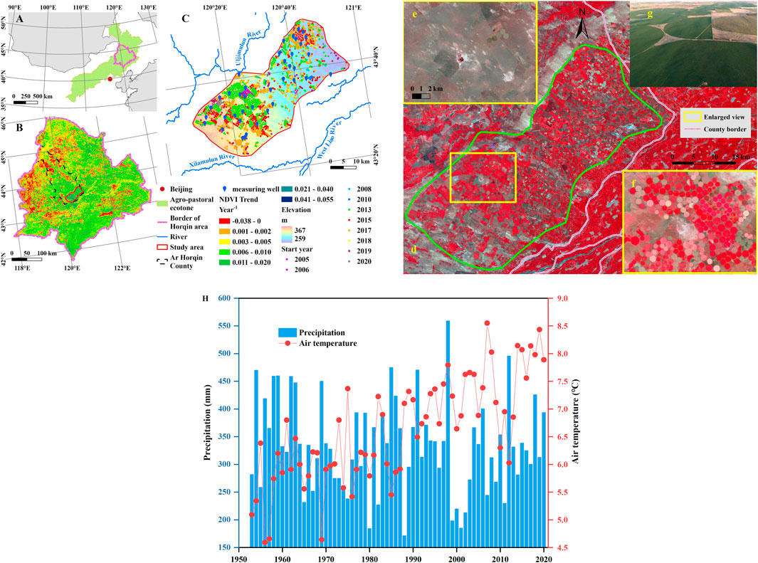
FIGURE 1. Location and spatial characteristics of the study area. (A) The Horqin area is in the southeastern part of northern China‘s agro-pastoral ecotone. (B) Change rate of the normalized difference vegetation index (NDVI) in the Horqin area from 2000 to 2021. (C) The distribution of center-pivot irrigation systems that were implemented from 2005 to 2020. (D) Landsat image of the study area in 2020, with magnification of local Landsat images in 2005 (E) and 2015 (F), and an aerial photograph of a center-pivot irrigation system (G). (H) The interannual dynamics of precipitation and air temperature in the past half century from a national reference climatological station (43°36′ 0″ N, 121°16′58.8″ E) approximately 45 km east of the study area A, B.

The study area has a temperate continental semi-arid monsoonal climate, with a mean annual temperature of 5.5°C (mean monthly temperatures ranging from -12.8°C in January to 23.4°C in August) and total annual precipitation of 368 mm (www.resdc.cn), of which 75% falls during the growing season from June to September. The total annual potential evaporation is 1800–2000 mm (Zhao et al., 2009). The elevation ranges from 259 to 367 m asl (Jarvis et al., 2008).

2.2 Geology and Hydrogeology

Geologically, the study area belongs to the subsidence zone from the Greater Khingan Mountains to the western Songliao Plain of China, and the paleosol and aeolian sand form interlayers. The underlying strata are loose alluvial and aeolian sediments of Quaternary, mainly medium and fine sand (diameter of 0.10–0.50 mm) in the various cracks with relatively high-water content or reserves. The thickness of the sedimentary layer varies from about 100 to 200 m (Qiu, 1989). The dominant zonal soils of this area are Arenosols mainly degraded from Kastanozems and Chernozems based on the taxonomy of the World Reference Base for Soil Resources (IUSS Working Group WRB, 2006).

Hydrologically, water resource is relatively rich mainly from the Yanshan Mountains and the Greater Khingan Mountains. The large part of available groundwater resource is shallow phreatic water in the aeolian sediments (Qiu, 1989), and recharged by precipitation, river runoff. The groundwater discharge is mainly to artificial wells for irrigation and daily use (Zhong et al., 2018).

2.3 Groundwater Level Measurements

The groundwater level in wells was measured using a water-stage recorder. The recorder is a 30-m steel ruler, wrapped with electric wire in a plastic shell and coiled around a hand wheel. A 10-cm stainless-steel probe is connected at the start of the tick marks on the ruler. The weight of the probe keeps the ruler perpendicular while it is inside the well. When the probe touches the water surface, a buzzer on the hand wheel sounds; when the probe is removed from the water, the buzzer stops immediately. The tick marks on the ruler from the ground surface represents the depth of the groundwater level. However, most of the gaps between the well edge and the pumping pipe of a CPI system are too narrow for the probe to enter or to reach the water surface inside the well, so it was not possible to measure in all wells. Although there are thousands of wells in this area, we were only able to find 42 irrigation wells at representative locations where we could monitor GL spatially from April 2019 to April 2022, including both CPI wells and conventional irrigation wells that without CPI system (Figure 1C). During our monthly monitoring in 2019, we found it difficult to measure all the target wells at normal level in same period (t) by excluding the lag effect of pumping, because there were sharp decreases which corresponded to GL measurements after an irrigation event. Since 2020, we have only monitored GL at the beginning of the irrigation period (in early April) and at the end (in Mid-October). We calculated the changes in GL (ΔGL) during discharge (irrigation) and subsequent recharge as follows:

$\mathrm{\Delta }G{L}_{\mathrm{discharge}}=G{L}_{t2}-G{L}_{t1}(1)$

$\mathrm{\Delta }G{L}_{\mathrm{recharge}}=G{L}_{t3}-G{L}_{t2}(2)$

where $\mathrm{\Delta }GL$ > 0 indicates groundwater discharge (irrigation) and decreased GL and ΔGL < 0 indicates groundwater recharge and increased GL; t₁ and t₂ represent the beginning and end of the monitoring in a given year, and t₃ represents the beginning of the following year. Therefore, t₁ to t₂ is the groundwater discharge (irrigation) period, t₂ to t₃ is the groundwater recharge period. The 42 (N) measuring wells were divided into three groups according to the normal GL: shallower (n1 = 9), <10 m; medium (n2 = 19), >10 m and <20 m; deeper (n3 = 14), >20 m.

2.4 Irrigation Intensity of Center-Pivot Irrigation Systems

The irrigation method in this study area is basically unified, i.e., the automatic sprinkler irrigation through tube wells of CPI systems. Thus, density of irrigation well can serve as a reasonable proxy for irrigation intensity. In addition, the change in cropping intensity (Duarte and Mateos, 2022) from natural to artificial ecosystems can validate the increased irrigation intensity.

2.4.1 Density of Irrigation Well

To identify irrigation intensity by well density, Landsat 5 TM images (2005, 2006, 2008, and 2010) and Landsat 8 OLI images (2013, 2015, 2017, 2019, and 2020) were obtained from the global visualization viewer of United States Geological Survey (https://glovis.usgs.gov/). The images were obtained in July or August. We also obtained Gaofen-1 satellite images (2018) in August from the Geospatial Data Cloud site, Computer Network Information Center, Chinese Academy of Sciences (https://www.gscloud.cn). The spatial resolutions were 30 m for the Landsat images, and 2 m for the Gaofen images. All images were overlaid in ArcGIS Pro (www.esri.com) to locate the center of each CPI well in time series. We assembled 1,598 wells of existing CPI systems and estimated the kernel density in 2000, 2005, 2010, 2015, and 2020 to allow monitoring of the changes over time.

Kernel density estimation is a mathematical technique that calculates the magnitude of density in space based on the detection of point or polyline features (ESRI Inc., 2020). The analysis uses a kernel function to fit a smoothly tapered response surface that provides an estimate of the probability-density function. It can be expressed mathematically as follows:

$\widehat{f}\left(x\right)=\frac{1}{n}{\displaystyle \sum }_{i=1}^{n}K\left(\frac{x-x_i}{h}\right)(3)$

where x_i (i = 1, 2, …, n) is the i-th sample point. x–x_i is the distance of that observation from a particular point x, K_h(x) is the chosen kernel function, and h is the bandwidth (Wglarczyk, 2018). For more details, please see https://mathisonian.github.io/kde/.

2.4.2 Cropping Intensity

Cropping intensity was measured in terms of normalized difference vegetation index (NDVI, regional) and aboveground biomass (plot) for the change from natural grassland to cultivated pasture.

For the NDVI dataset, we used the MODIS/Terra Vegetation Indices product (MOD13Q1), which has a 16-day repeat cycle and a 250-m spatial resolution (Didan, 2015). The data was obtained by using the Application for Extracting and Exploring Analysis Ready Samples (AρρEEARS), which offers an efficient way to access and transform geospatial data through area samples by extracting polygons that can be used in GIS software (https://lpdaacsvc.cr.usgs.gov/appeears/). Annual NDVI sequences were derived from all 16-day values for each year from 2000 to 2021. We used the annual maximum NDVI, which were obtained by maximum value compositing method.

We extracted annual NDVI values related to the locations of each CPI system, respectively, divided into two periods by the start year of implementing CPI (Figure 1C), i.e., NDVI_NG (natural grassland, values before the start year) and NDVI_CP (cultivated pasture, values from the start year). Note that in this comparison, “NG” refers to all years before the start year, and “CP” refers to all years from the start year, rather than a single year.

Ordinary least-squares regression is frequently used to describe the variation within a sequence of data. In this study, we analyzed the NDVI trends for individual pixels in our study area using the following formula:

${\text{Θ}}_{\text{slope}}=\frac{(n\times {{\displaystyle \sum }}_{i=1}^{n}i\times NDV{I}_i)-\left({{\displaystyle \sum }}_{i=1}^{n}i\right)\left({{\displaystyle \sum }}_{i=1}^{n}NDV{I}_i\right)}{n\times {{\displaystyle \sum }}_{i=1}^n{i}^2-{\left({{\displaystyle \sum }}_{i=1}^{n}i\right)}^2}(4)$

where Θ_slope is the slope of the linear regression equation; NDVI_i is the annual maximum value in the ith year; and n is the number of years in the study period (here, between 2000 and 2021). Θ_slope < 0 represent a decrease in NDVI during the period, whereas Θ_slope > 0 represent an increase (Lian et al., 2017).

We measured the live aboveground biomass before mowing in late August, including both natural grassland (8 plots) and cultivated pasture irrigated by a CPI system (Figures 1D–G, 11 plots, 5 for Avena species and 6 for Medicago sativa) in different parts of the study area. We randomly established three quadrats (each 1 × 1 m) in each plot. All the aboveground living biomass was harvested by mowing method in each quadrat, and taken to the laboratory for oven-drying at 70°C to a constant weight (Ni, 2004).

2.5 Statistical and Prediction Methods

2.5.1 Regression Kriging for Prediction of Spatial Groundwater Level

Regression kriging combines least-squares regression with simple kriging to analyze both the trend term µ(x) of the least-squares regression (non-geostatistical) with the residual term ε’(x) from the geostatistical analysis:

$Z\left(x\right)=\mu \left(x\right)+{\epsilon }^{\prime }\left(x\right)+{\epsilon }^{″}\left(x\right)(5)$

where Z(x) and ε''(x) represent the random variable Z and the unexplained variation at location x, respectively (Keskin and Grunwald, 2018). We used the geostatistical wizard provided by ArcGIS Pro (www.esri.com) to perform prediction of the depth of GL and ΔGL by combining empirical Bayesian kriging with the explanatory raster data of elevation. The elevation data was obtained from the Shuttle Radar Telemetry Mission DEM product (Jarvis et al., 2008). This approach provides a more reliable estimate than other kriging methods, because it accounts for the uncertainty of semivariogram estimation (ESRI Inc., 2020).

We also estimated the theoretical minimums of energy consumption when pumping through wells of CPI systems. It was the increase in gravitational potential energy (ΔGPE > 0, Joule) per unit mass of groundwater (e.g., 100 kg) that pumped to the ground surface (Tan, 2008) during 2019–2021, based on the spatial prediction of the depth of GL.

$\mathrm{W}=\mathrm{\Delta }\mathit{GPE=m}\times \mathit{g}\times \mathrm{\Delta }h(6)$

where m (kg), g (9.8 m s⁻²), and Δh (m) represent the mass of groundwater, gravitational acceleration (constant, without considering the slight change during vertical displacement), and the displacement of the groundwater (distance from GL to the ground), respectively.

2.5.2 Statistical Methods

We used paired-sample t-tests (with significance at p < 0.01) to compare NDVI_NG and NDVI_CP, and used Duncan’s new multiple-range test (with significance at p < 0.05) to perform one-way ANOVA to reveal differences of ΔGL of measuring well between three groups, and aboveground biomass between natural and cultivated pasture. We have natural-logarithm-transformed the variables which didn’t pass the Kolmogorov–Smirnov test (p < 0.05).

3 Results

3.1 Spatial and Temporal Dynamics of Well Density of Center-Pivot Irrigation System

Based on the satellite images, Table 1 showed that the implementation of CPI systems went through an exploratory stage from 2005 to 2012, followed by rapid expansion, reaching great peaks in 2013, 2015, and 2017, respectively, with 539, 308, and 573 new wells added, accounting for 88.9% of the total number during the study period. Figure 2 showed the changes in the spatial pattern of CPI wells over four 5-year periods. The land use type was natural grassland with few irrigation facilities before 2005 (Figure 2A and Table 1). In 2005, CPI started at only two locations, with well densities of 0.16 and less than 0.10 km⁻² (Figure 2B). From 2005 to 2010, CPI still developed slowly with the highest well density (0.64 km⁻²) in the middle of the study area (Figure 2C). Then, the density increased rapidly between 2013 and 2015, from 0.64 to 2.52 wells km⁻² and formed multiple hotspots (Table 1 and Figure 2D). From 2015 to 2020, the multiple hotspots combined to form contiguous CPI area in the southern part of the study area, and two large centers (>1.01 and 2.31 wells km⁻²) appeared in the northern part (Figure 2E). Thus, the gaps were shrinking between CPI wells as the area of higher well density expanding.

TABLE 1

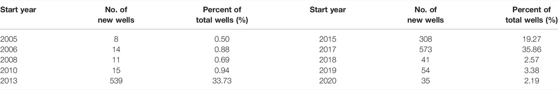
TABLE 1. Changes in the number of new center-pivot irrigation wells.

FIGURE 2

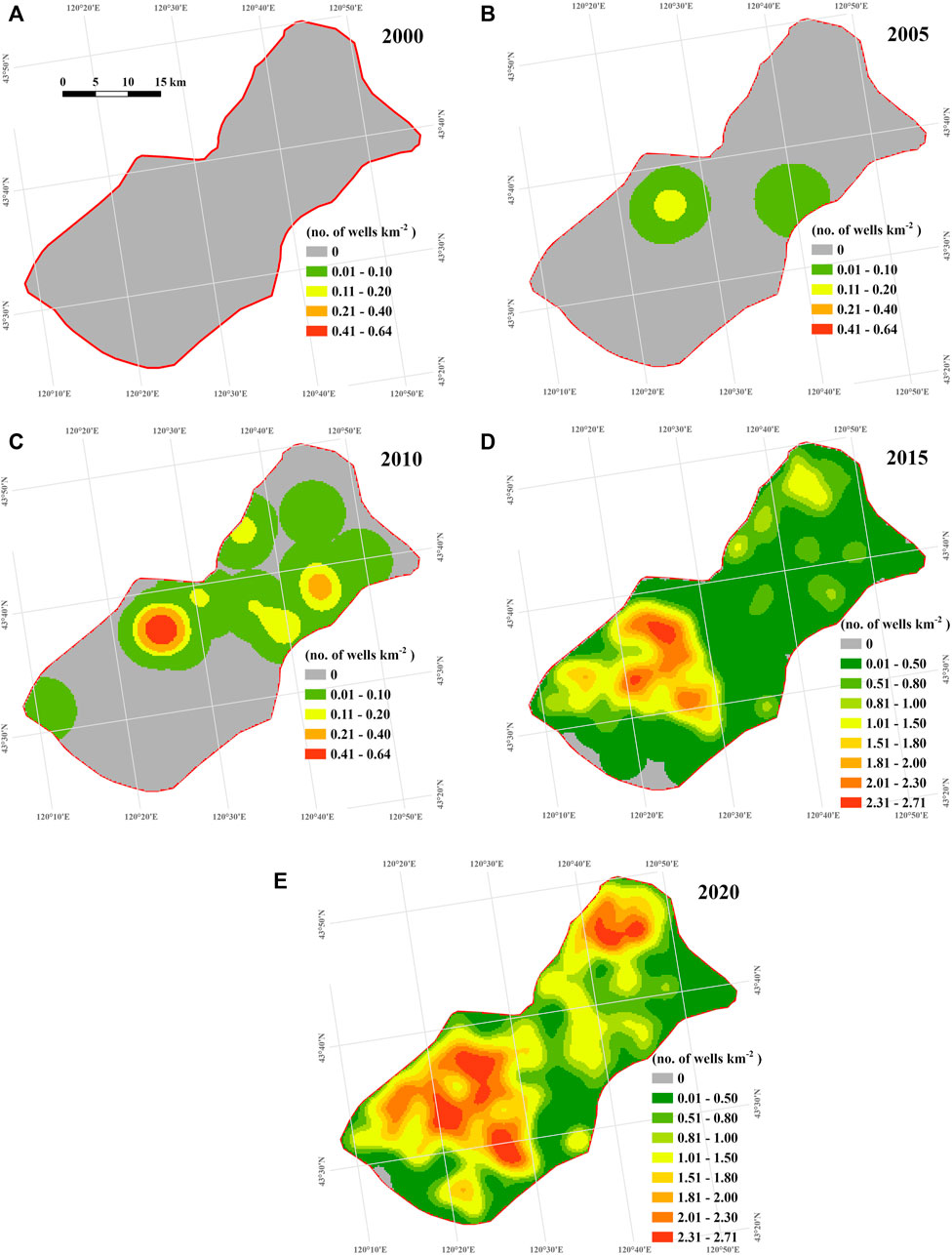
FIGURE 2. Kernel density estimates for the center-pivot irrigation wells. (A) 2000, (B) 2005, (C) 2010, (D) 2015, and (E) 2020.

3.2 Groundwater Level Dynamics at Different Depths

The GL trends of the three groups were basically the same during the monitoring time from 2019 to 2022 (Supplementary Figure S1). The changes in ΔGL indicated that the discharge of groundwater accelerated as the normal GL decreased, because the averaged ΔGL in the deeper group (0.94 m for GL > 20 m) was significantly higher than those of the shallower group (0.64 m for GL < 10 m) and medium group (0.73 m for 10 m < GL < 20 m) (Figure 3A). During groundwater recharge period, the averaged ΔGL in the deeper (−0.29 m) and medium groups (−0.29 m) were significantly higher than that in the shallower group (−0.12 m) (Figure 3B). Combined the two periods (Figures 3A,B), it revealed that the deeper group showed a significantly greater net decrease (0.63 m yr⁻¹) than the shallower group (0.38 m yr⁻¹) and medium group (0.43 m yr⁻¹) (Figure 3C).

FIGURE 3

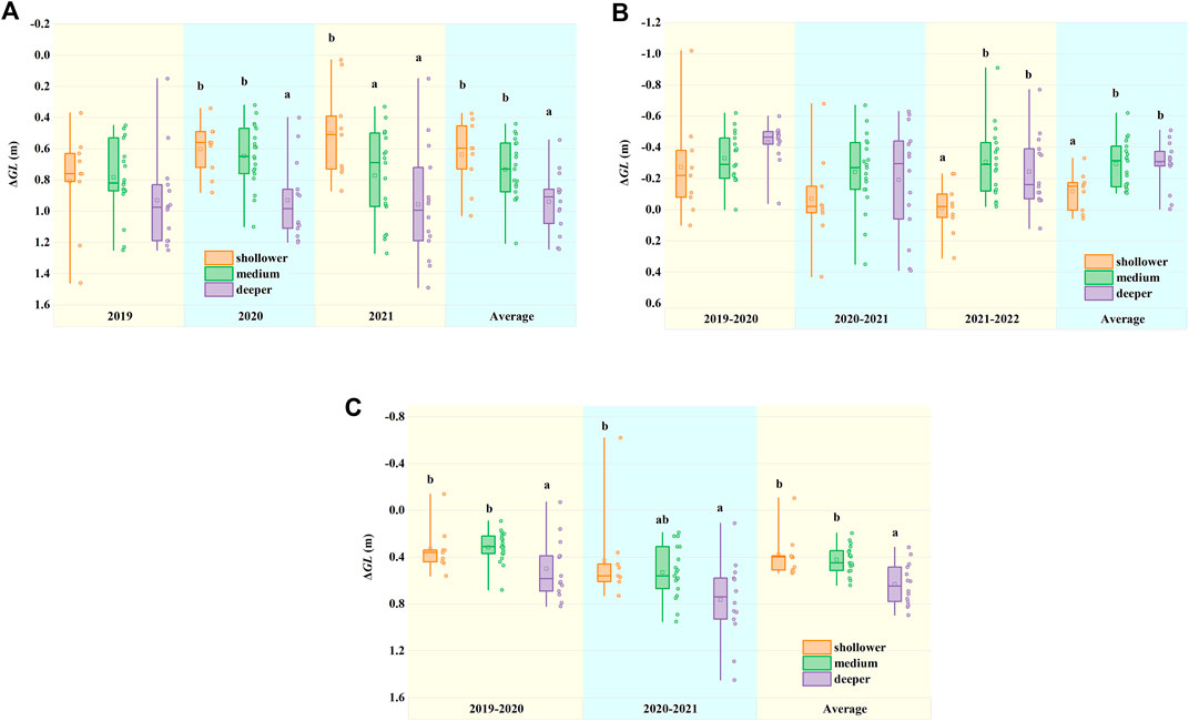
FIGURE 3. Change in the groundwater level (ΔGL) from 2019 to 2022. Box-whisker plots show the mean (square), median (solid line) in the boxes, and the 5th and 95th percentiles on the whiskers. (A) The groundwater discharge (irrigation) period, with ΔGL from April to October within the year; (B) The groundwater recharge period, with ΔGL from October to the following April; and (C) ΔGL_interannual, which represents the net change from October to the following October. The statistical significances are marked with lowercase letters (p < 0.05).

3.3 Relationships Between Groundwater Level and Well Density of Center-Pivot Irrigation System

Regression kriging was used to predict the spatial patterns of ΔGL and GL, which were significantly and positively (R² = 0.447 and 0.429, p < 0.001, Supplementary Table S1) correlated with the well density (kernel density) of CPI system, respectively. It showed a fitted plane function in the 3D coordinate system based on the variables (R² = 0.655, p < 0.001, Figure 4). The predicted trend of GL was consistent with the observed change, and indicated a significant positive linear relationship between ΔGL and GL (R² = 0.612, p < 0.001, Supplementary Table S1). Therefore, ΔGL was determined by the both well density and the depth of GL.

FIGURE 4

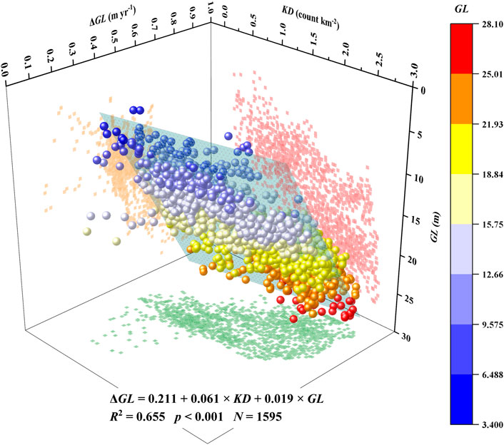
FIGURE 4. Relationships among ΔGL (the change of the groundwater level from April 2019 to October 2021), KD (kernel density in 2020), and GL (the mean in Octobers). Each sphere represented a CPI well. The plane function is represented as z = z₀ + a*x + b*y, and all parameters of z₀, a, and b are significant (p < 0.001).

4 Discussion

4.1 Cropping Intensity Affect Irrigation Intensity in the Agro-Pastoral Ecotone

Cropping intensity represents the combination of agricultural water use and land use patterns, which can directly associate with irrigation intensity. It is determined by agricultural policies, social-economic factors, and farmers’ subjective wishes (Duarte and Mateos, 2022). As more than 60% of the water area has shrunk in the Horqin area (Tao et al., 2015), the use of well irrigation has expanded rapidly since 2000 and the groundwater-based irrigation is increasing year by year to make up for the lack of rainfall and surface water (Zhong et al., 2018). A 2013 questionnaire survey in the middle of the agro-pastoral ecotone (around the Yinshan Mountains) showed that 31% of the local farmers had turned dry land into irrigated land (Wang et al., 2020).

Stable water availability is considered as the most critical guarantees for crop production (Auci and Vignani, 2021), particularly in agricultural areas with frequent drought (Bryan et al., 2013; Khan et al., 2021). Our kernel density results suggested that the implementation of high-density, high-efficiency, and large-scale CPI systems initiated a new mode of land-use change. Both the regional NDVI and quadrat-based survey indicated that the cropping intensity was significantly enhanced (p < 0.01) after implementation of CPI systems, as shown between natural grassland and cultivated pastures (Figures 5A,B and Table 2). The NDVI_CP was significantly higher than the NDVI_NG (p < 0.01), with an increase of 30.6%–59.2%. The aboveground biomass of Avena species (503.6 ± 40.7 g m⁻²) and Medicago sativa (270.0 ± 7.6 g m⁻²) were significantly higher (p < 0.01) than that of natural grassland (182.2 ± 11.1 g m⁻²) by 176.4% and 48.7%, respectively. Due to the difference in cropping intensity, the CPI area was clearly separated from the non-irrigated area, because the NDVI_slope of non-irrigated area was much lower than that of CPI area, even showing a negative trend of slight degradation (Figure 5C).

FIGURE 5

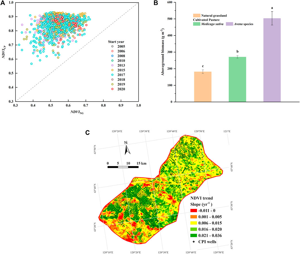
FIGURE 5. Comparison of the normalized difference vegetation index (NDVI) and aboveground biomass between natural grassland (NG) and cultivated pasture (CP). (A) Relationship between NDVI_NG and NDVI_CP divided by the start year of irrigation (NDVI_NG, values before the start year, natural grassland; NDVI_CP, values from the start year, cultivated pasture, e.g., 2010 represents the mean from 2010 to 2021). (B) Differences in aboveground biomass between natural grassland and the cultivated pastures. (C) Trend of NDVI (NDVI_slope) from 2000 to 2021 related to the locations of the center-pivot irrigation (CPI) wells.

TABLE 2

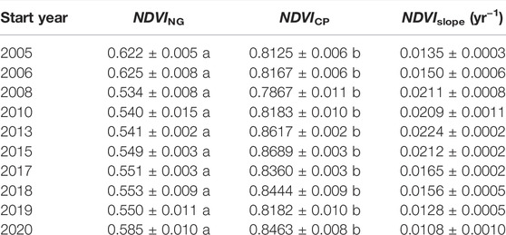
TABLE 2. Changes in the normalized difference vegetation index (NDVI) between natural grassland (NG) and cultivated pasture (CP). NDVI values (mean ± SE) are labeled with different letters for significance (t-test, p < 0.01). The NDVI_slope represents NDVI trend from 2000 to 2021.

4.2 Risks and Countermeasures of Groundwater Depletion Based on Irrigation Intensity

GL is generally affected by the dynamic balance between the recharge and discharge to aquifer storage, including natural (Liu et al., 2022) and anthropogenic factors (Zencich et al., 2002; Seeyan et al., 2014). The causes of ΔGL are always complex from shallow to deep aquifers, including rainfall and evapotranspiration (Bai et al., 2017), irrigated area and cost (Foster et al., 2015), and effectiveness of water-saving approaches and sustainable water management (Malki et al., 2017; Salem et al., 2017). Sustainable use of irrigation water aims to increase crop yields with less water input by improved water management efficiency (Chartzoulakis and Bertaki, 2015). In our study area, the observed ΔGL was mainly caused by human activities. It was consistent with the trend (1975–2000) that had been reported for the Hebei plains in northern China, where the ΔGL ranged from 0.42 m yr⁻¹ to more than 1.21 m yr⁻¹, respectively, in shallow and deep aquifers (Duan and Xiao, 2003). The ΔGL at different depths suggested that shallow groundwater may be relatively susceptible to replenishment by rainfall and subsurface flow (Xie et al., 2011; Gao et al., 2015), while deep groundwater was more sensitive to water withdraw for irrigation (Russo and Lall, 2017).

Our study is also a typical case that related in water–energy–food nexus. The direct consequence of groundwater depletion is the increase in energy consumption for pumping. As more than 1,500 pumps have different power ratings and working hours, we roughly estimated the energy consumption for irrigation (14,521.7 J on average) in terms of change in gravitational potential energy (ΔGPE) of water (each 100 kg equals to 100 mm water m⁻², Figure 6A). Excessive density of CPI wells (deeper GL) not only led to a dramatic increase in the risk of unsustainable water use, but also increase energy consumption at a rate of over 800 J yr⁻¹ per 100 kg water (Figure 6B). Left unchecked, underpowered submersible pumps will have to be replaced, with irreversible effects on irrigation costs.

FIGURE 6

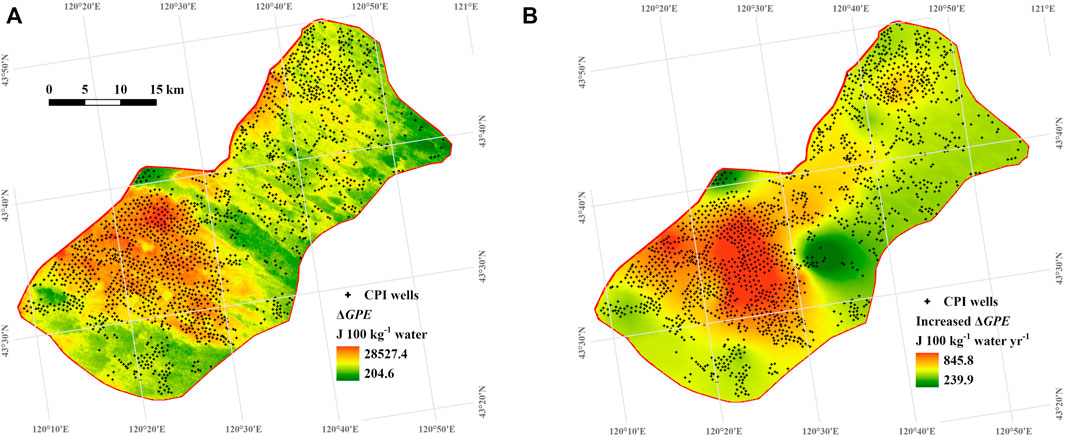
FIGURE 6. Change in gravitational potential energy (ΔGPE) during 2019–2021. (A) Spatial pattern of ΔGPE from the average groundwater level in October to ground. (B) Increased ΔGPE based on averaged ΔGL (the change of the groundwater level). CPI, center-pivot irrigation.

According to our results (Figure 4), if the well density remains unchanged, and the depth of GL increase by 10 m, the ΔGL will increase by about 0.19 m yr⁻¹; if GL is maintained at the same depth and the well density increases by 1.0 count km⁻², the ΔGL will increase by about 0.06 m yr⁻¹. However, a limitation of our results is that it can only interpret the ΔGL pattern in recent years; whereas the current status of regional depth of GL should be the result of well density and its long-term changes. Thus, some studies believe that an appropriate water price can prompt users to conserve water and use water-saving technologies (Auci and Vignani, 2021). At the same time, excessively dense wells should be adjusted (e.g., kept within 0.5 count km⁻²). Compared to Avena species, Medicago sativa (perennial) should be recommended to reduce both water consumption and soil tillage. Water use mode in the past should be changed by new irrigation schedule, and further research is needed on water use efficiency of cultivated pasture.

5 Conclusion

This study preliminarily attempted to explore the effect of regional intensity of center-pivot irrigation on groundwater level at different depths. From the perspective of land use change since 2000, the implementation of high-density, high-efficiency, and large-scale CPI system has significantly enhanced the regional irrigation intensity. The deeper groundwater was more sensitive to water withdrawal for irrigation than that of shallower groundwater because of the different well densities.

The combination of intensive agricultural water use and land use creates the potential risks of unsustainable water availability, which could dramatically increase irrigation costs in the foreseeable future. Water resource managers should strictly control the density of center-pivot irrigation systems, adjust irrigation schedule and forage varieties in hotspot areas, and ensure the sustainable availability of groundwater.

Data Availability Statement

All datasets generated for this study are included in the article/Supplementary Material. For further inquiries, please contact the corresponding author or the first author.

Author Contributions

All co-authors contributed to the manuscript. JL, YLL, and YQL designed and performed the experiments. XZ and TZ conceived the experiments, and modified the manuscript. XiW, XuW, LW, and RZ were responsible for data observation, collection, and processing of the materials. JL, YLL, and YQL processed and analysed the data, and wrote this paper.

Funding

This study was financially supported by the National Natural Science Foundation of China (grant 41807525), the Key Science and Technology Program of Inner Mongolia (grant 2021ZD0015), the National Natural Science Foundation of China (grant 42177456 and 31971466), and the National Basic Resources Survey Project of China (grant 2017FY100200).

Conflict of Interest

The authors declare that the research was conducted in the absence of any commercial or financial relationships that could be construed as a potential conflict of interest.

Publisher’s Note

All claims expressed in this article are solely those of the authors and do not necessarily represent those of their affiliated organizations, or those of the publisher, the editors and the reviewers. Any product that may be evaluated in this article, or claim that may be made by its manufacturer, is not guaranteed or endorsed by the publisher.

Acknowledgments

We thank our colleagues at the Naiman Desertification Research Station, Chinese Academy of Sciences, for their help with the field investigation. We thank the journal’s reviewers for their constructive comments on the manuscript.

Supplementary Material

The Supplementary Material for this article can be found online at: https://www.frontiersin.org/articles/10.3389/fenvs.2022.892577/full#supplementary-material

References

Auci, S., and Vignani, D. (2021). Irrigation Water Intensity and Climate Variability: An Agricultural Crops Analysis of Italian Regions. Environ. Sci. Pollut. Res. 28, 63794–63814. doi:10.1007/s11356-020-12136-6

CrossRef Full Text | Google Scholar

Bai, L., Cai, J., Liu, Y., Chen, H., Zhang, B., and Huang, L. (2017). Responses of Field Evapotranspiration to the Changes of Cropping Pattern and Groundwater Depth in Large Irrigation District of Yellow River Basin. Agric. Water Manag. 188, 1–11. doi:10.1016/j.agwat.2017.03.028

CrossRef Full Text | Google Scholar

Bryan, E., Ringler, C., Okoba, B., Roncoli, C., Silvestri, S., and Herrero, M. (2013). Adapting Agriculture to Climate Change in Kenya: Household Strategies and Determinants. J. Environ. Manag. 114, 26–35. doi:10.1016/j.jenvman.2012.10.036

PubMed Abstract | CrossRef Full Text | Google Scholar

Chartzoulakis, K., and Bertaki, M. (2015). Sustainable Water Management in Agriculture under Climate Change. Agric. Agric. Sci. Procedia 4, 88–98. doi:10.1016/j.aaspro.2015.03.011

CrossRef Full Text | Google Scholar

Cheng, G., Li, X., Zhao, W., Xu, Z., Feng, Q., Xiao, S., et al. (2014). Integrated Study of the Water-Ecosystem-Economy in the Heihe River Basin. Natl. Sci. Rev. 1, 413–428. doi:10.1093/nsr/nwu017

CrossRef Full Text | Google Scholar

Didan, K. (2015). MOD13Q1 MODIS/Terra Vegetation Indices 16-Day L3 Global 250m SIN Grid. Washington, DC: NASA EOSDIS Land Processes DAAC, v006. doi:10.5067/MODIS/MOD13Q1.006

CrossRef Full Text | Google Scholar

Döll, P., Hoffmann-Dobrev, H., Portmann, F. T., Siebert, S., Eicker, A., Rodell, M., et al. (2012). Impact of Water Withdrawals from Groundwater and Surface Water on Continental Water Storage Variations. J. Geodyn. 59-60, 143–156. doi:10.1016/j.jog.2011.05.001

CrossRef Full Text | Google Scholar

Duan, Y. H., and Xiao, G. Q. (2003). Sustainable Utilization of Groundwater Resources in Hebei Plain. Hydrogeology Eng. Geol., 2–8. (In Chinese). doi:10.3969/j.issn.1000-3665.2003.01.002

CrossRef Full Text | Google Scholar

Duarte, A. C., and Mateos, L. (2022). How Changes in Cropping Intensity Affect Water Usage in an Irrigated Mediterranean Catchment. Agric. Water Manag. 260, 107274. doi:10.1016/j.agwat.2021.107274

CrossRef Full Text | Google Scholar

EEA (2021). Water Resources across Europe—Confronting Water Scarcity and Drought. Copenhagen, Denmark. EEA Report No 12/2021.

Google Scholar

ESRI Inc. (2020). ArcGIS Pro Help. California, USA: Redlands.

Google Scholar

Famiglietti, J. S. (2014). The Global Groundwater Crisis. Nat. Clim. Change 4, 945–948. doi:10.1038/nclimate2425

CrossRef Full Text | Google Scholar

Fan, Y., Li, H., and Miguez-Macho, G. (2013). Global Patterns of Groundwater Table Depth. Science 339, 940–943. doi:10.1126/science.1229881

PubMed Abstract | CrossRef Full Text | Google Scholar

FAO (2017). The Future of Food and Agriculture – Trends and Challenges. Rome.

Google Scholar

Foster, T., Brozović, N., and Butler, A. P. (2015). Analysis of the Impacts of Well Yield and Groundwater Depth on Irrigated Agriculture. J. Hydrology 523, 86–96. doi:10.1016/j.jhydrol.2015.01.032

CrossRef Full Text | Google Scholar

Gao, X., Huo, Z., Bai, Y., Feng, S., Huang, G., Shi, H., et al. (2015). Soil Salt and Groundwater Change in Flood Irrigation Field and Uncultivated Land: A Case Study Based on 4-year Field Observations. Environ. Earth Sci. 73, 2127–2139. doi:10.1007/s12665-014-3563-4

CrossRef Full Text | Google Scholar

Hu, X., Shi, L., Zeng, J., Yang, J., Zha, Y., Yao, Y., et al. (2016). Estimation of Actual Irrigation Amount and its Impact on Groundwater Depletion: A Case Study in the Hebei Plain, China. J. Hydrology 543, 433–449. doi:10.1016/j.jhydrol.2016.10.020

CrossRef Full Text | Google Scholar

IUSS Working Group WRB (2006). World Reference Base for Soil Resources 2006—a Framework for International Classification, Correlation and Communication, 103. Rome: Food and Agriculture Organization of the United Nations.

Google Scholar

Jarvis, A., Reuter, H. I., Nelson, A., and Guevara, E. (2008). Hole-filled SRTM for the Globe Version 4. CGIAR-CSI SRTM 90m Database. Available at: https://cgiarcsi.community/data/srtm-90m-digital-elevation-database-v4-1/.

Google Scholar

Keskin, H., and Grunwald, S. (2018). Regression Kriging as a Workhorse in the Digital Soil Mapper's Toolbox. Geoderma 326, 22–41. doi:10.1016/j.geoderma.2018.04.004

CrossRef Full Text | Google Scholar

Khan, M. Y. A., El Kashouty, M., Gusti, W., Kumar, A., Subyani, A. M., and Alshehri, A. (2022). Geo-Temporal Signatures of Physicochemical and Heavy Metals Pollution in Groundwater of Khulais Region-Makkah Province, Saudi Arabia. Front. Environ. Sci. 9, 800517. doi:10.3389/fenvs.2021.800517

CrossRef Full Text | Google Scholar

Khan, M. Y. A., Elkashouty, M., Subyani, A. M., Tian, F., and Gusti, W. (2021). GIS and RS Intelligence in Delineating the Groundwater Potential Zones in Arid Regions: A Case Study of Southern Aseer, Southwestern Saudi Arabia. Appl. Water Sci. 12, 3. doi:10.1007/s13201-021-01535-w

CrossRef Full Text | Google Scholar

Konikow, L. F. (2013). Groundwater Depletion in the United States (1900–2008). Washington, DC: United States Geological Survey.

Google Scholar

Lian, J., Zhao, X., Li, X., Zhang, T., Wang, S., Luo, Y., et al. (2017). Detecting Sustainability of Desertification Reversion: Vegetation Trend Analysis in Part of the Agro-Pastoral Transitional Zone in Inner mongolia, china. Sustainability 9, 211. doi:10.3390/su9020211

CrossRef Full Text | Google Scholar

Liu, X., He, Y., Sun, S., Zhang, T., Luo, Y., Zhang, L., et al. (2022). Restoration of Sand-Stabilizing Vegetation Reduces Deep Percolation of Precipitation in Semi-arid Sandy Lands, Northern China. Catena 208, 105728. doi:10.1016/j.catena.2021.105728

CrossRef Full Text | Google Scholar

Malki, M., Bouchaou, L., Hirich, A., Ait Brahim, Y., and Choukr-Allah, R. (2017). Impact of Agricultural Practices on Groundwater Quality in Intensive Irrigated Area of Chtouka-Massa, Morocco. Sci. Total Environ. 574, 760–770. doi:10.1016/j.scitotenv.2016.09.145

PubMed Abstract | CrossRef Full Text | Google Scholar

Ni, J. (2004). Estimating Net Primary Productivity of Grasslands from Field Biomass Measurements in Temperate Northern China. Plant Ecol. 174, 217–234. doi:10.1023/B:VEGE.0000049097.85960.10

CrossRef Full Text | Google Scholar

OECD (2012). The OECD Environmental Outlook to 2050: The Consequences of Inaction. Paris: OECD.

Google Scholar

O’Shaughnessy, S. A., and Rush, C. (2014). “Precision Agriculture: Irrigation,” in Encyclopedia of Agriculture and Food Systems. Editor N. K. Van Alfen (Oxford: Academic Press), 521–535. doi:10.1016/B978-0-444-52512-3.00235-7

CrossRef Full Text | Google Scholar

Qiu, S. (1989). Study on the Formation and Evolution of Horqin Sandy Land. Sci. Geogr. Sin. 9, 317–328.

Google Scholar

Ravenscroft, P., and Lytton, L. (2022). Seeing the Invisible : A Strategic Report on Groundwater Quality. Washington, D.C: World Bank.

Google Scholar

Russo, T. A., and Lall, U. (2017). Depletion and Response of Deep Groundwater to Climate-Induced Pumping Variability. Nat. Geosci. 10, 105–108. doi:10.1038/ngeo2883

CrossRef Full Text | Google Scholar

Salem, G. S. A., Kazama, S., Komori, D., Shahid, S., and Dey, N. C. (2017). Optimum Abstraction of Groundwater for Sustaining Groundwater Level and Reducing Irrigation Cost. Water Resour. Manage 31, 1947–1959. doi:10.1007/s11269-017-1623-8

CrossRef Full Text | Google Scholar

Scanlon, B. R., Faunt, C. C., Longuevergne, L., Reedy, R. C., Alley, W. M., Mcguire, V. L., et al. (2012). Groundwater Depletion and Sustainability of Irrigation in the US High Plains and Central Valley. Proc. Natl. Acad. Sci. U.S.A. 109, 9320–9325. doi:10.1073/pnas.1200311109

PubMed Abstract | CrossRef Full Text | Google Scholar

Scanlon, B. R., Reedy, R. C., Gates, J. B., and Gowda, P. H. (2010). Impact of Agroecosystems on Groundwater Resources in the Central High Plains, USA. Agric. Ecosyst. Environ. 139, 700–713. doi:10.1016/j.agee.2010.10.017

CrossRef Full Text | Google Scholar

Schyns, J. F., Hoekstra, A. Y., Booij, M. J., Hogeboom, R. J., and Mekonnen, M. M. (2019). Limits to the World's Green Water Resources for Food, Feed, Fiber, Timber, and Bioenergy. Proc. Natl. Acad. Sci. U.S.A. 116, 4893–4898. doi:10.1073/pnas.1817380116

PubMed Abstract | CrossRef Full Text | Google Scholar

Seeyan, S., Merkel, B., and Abo, R. (2014). Investigation of the Relationship between Groundwater Level Fluctuation and Vegetation Cover by Using NDVI for Shaqlawa Basin, Kurdistan Region - Iraq. Jgg 6, 187–202. doi:10.5539/jgg.v6n3p187

CrossRef Full Text | Google Scholar

Siebert, S., Burke, J., Faures, J. M., Frenken, K., Hoogeveen, J., Döll, P., et al. (2010). Groundwater Use for Irrigation - a Global Inventory. Hydrol. Earth Syst. Sci. 14, 1863–1880. doi:10.5194/hess-14-1863-2010

CrossRef Full Text | Google Scholar

Tan, A. (2008). “Newton's Law of Gravitation,” in Theory of Orbital Motion. Editor A. Tan (World Scientific Publishing Company), 26–46. doi:10.1142/9789812709134_0002

CrossRef Full Text | Google Scholar

Tao, S., Fang, J., Zhao, X., Zhao, S., Shen, H., Hu, H., et al. (2015). Rapid Loss of Lakes on the Mongolian Plateau. Proc. Natl. Acad. Sci. U.S.A. 112, 2281–2286. doi:10.1073/pnas.1411748112

PubMed Abstract | CrossRef Full Text | Google Scholar

Wang, X., Zhang, B., Xu, X., Tian, J., and He, C. (2020). Regional Water-Energy Cycle Response to Land Use/cover Change in the Agro-Pastoral Ecotone, Northwest China. J. Hydrology 580, 124246. doi:10.1016/j.jhydrol.2019.124246

CrossRef Full Text | Google Scholar

Wglarczyk, S. (2018). Kernel Density Estimation and its Application. ITM Web Conf. 23, 00037. doi:10.1051/itmconf/20182300037

CrossRef Full Text | Google Scholar

Wu, B., Ma, Z., and Yan, N. (2020). Agricultural Drought Mitigating Indices Derived from the Changes in Drought Characteristics. Remote Sens. Environ. 244, 111813. doi:10.1016/j.rse.2020.111813

CrossRef Full Text | Google Scholar

Xie, T., Liu, X., and Sun, T. (2011). The Effects of Groundwater Table and Flood Irrigation Strategies on Soil Water and Salt Dynamics and Reed Water Use in the Yellow River Delta, China. Ecol. Model. 222, 241–252. doi:10.1016/j.ecolmodel.2010.01.012

CrossRef Full Text | Google Scholar

Zencich, S. J., Froend, R. H., Turner, J. V., and Gailitis, V. (2002). Influence of Groundwater Depth on the Seasonal Sources of Water Accessed by Banksia Tree Species on a Shallow, Sandy Coastal Aquifer. Oecologia 131, 8–19. doi:10.1007/s00442-001-0855-7

PubMed Abstract | CrossRef Full Text | Google Scholar

Zhao, H.-L., He, Y.-H., Zhou, R.-L., Su, Y.-Z., Li, Y.-Q., and Drake, S. (2009). Effects of Desertification on Soil Organic C and N Content in Sandy Farmland and Grassland of Inner Mongolia. Catena 77, 187–191. doi:10.1016/j.catena.2008.12.007

CrossRef Full Text | Google Scholar

Zhao, W., and Chang, X. (2014). The Effect of Hydrologic Process Changes on NDVI in the Desert-Oasis Ecotone of the Hexi Corridor. Sci. China Earth Sci. 57, 3107–3117. doi:10.1007/s11430-014-4927-z

CrossRef Full Text | Google Scholar

Zhong, Y., Zhong, M., Feng, W., Zhang, Z., Shen, Y., and Wu, D. (2018). Groundwater Depletion in the West Liaohe River Basin, china and its Implications Revealed by GRACE and In Situ Measurements. Remote Sens. 10, 493. doi:10.3390/rs10040493

CrossRef Full Text | Google Scholar