Acoustic Mapping of Gas Stored in Sediments of Shallow Aquatic Systems Linked to Methane Production and Ebullition Patterns

Bubble-mediated transport is the predominant pathway of methane emissions from inland waters, which are a globally significant sources of the potent greenhouse gas to the atmosphere. High uncertainties exist in emission estimates due to high spatial and temporal variability. Acoustic methods have been applied for the spatial mapping of ebullition rates by quantification of rising gas bubbles in the water column. However, the high temporal variability of ebullition fluxes can influence estimates of mean emission rates if they are based on reduced surveys. On the other hand, echo sounding has been successfully applied to detect free gas stored in the sediment, which provide insights into the spatial variability of methane production and release. In this study, a subtropical, midsize, mesotrophic drinking water reservoir in Brazil was investigated to address the spatial and temporal variability of free gas stored in the sediment matrix. High spatial resolution maps of gas content in the sediment were estimated from echo-sounding surveys. The gas content was analyzed in relation to water depth, sediment deposition, and organic matter content (OMC) available from previous studies, to investigate its spatial variability. The analysis was further supported by measurements of potential methane production rates, porewater methane concentration, and ebullition flux. The largest gas content (above average) was found at locations with high sediment deposition, and its magnitude depended on the water depth. At shallow water depth (<10 m), high methane production rates support gas-rich sediment, and ebullition is observed to occur rather continuously. At larger water depth (>12 m), the gas stored in the sediment is released episodically during short events. An artificial neural network model was successfully trained to predict the gas content in the sediment as a function of water depth, OMC, and sediment thickness (R² = 0.89). Largest discrepancies were observed in the regions with steep slopes and for low areal gas content (<4 L m⁻²). Although further improvements are proposed, we demonstrate the potential of echo-sounding for gas detection in the sediment, which combined with sediment and water body characteristics provides insights into the processes that regulate methane emissions from inland waters.

1 Introduction

Methane (CH₄) is a potent atmospheric greenhouse gas, whose concentration has increased nearly three-fold since pre-industrial times, primarily due to anthropogenic activity (IPCC, 2013; Saunois et al., 2020). Although CH₄ emissions represent only 3% of the anthropogenic carbon dioxide emissions in units of carbon mass flux, the increase in atmospheric CH₄ concentrations contribute ∼23% (∼0.62 W m⁻²) to the additional radiative forcing during the last century (Etminan et al., 2016). Recent estimates suggest that emissions from inland waters contribute nearly half of the total current CH₄ emissions from natural and anthropogenic sources (Rosentreter et al., 2021). These emissions represent the largest uncertainty in current CH₄ budgets (Saunois et al., 2020). Although freshwater CH₄ emissions are considered as natural sources, they are expected to increase in response to climate warming and to anthropogenic activities including cultural eutrophication and modifications of aquatic ecosystems (Pekel et al., 2016; DelSontro et al., 2018; Beaulieu et al., 2019; Peacock et al., 2021). Manmade reservoirs have been estimated to contribute 2–8% to freshwater CH₄ emissions (Deemer et al., 2016).

The estimation of methane emissions from inland waters is sensitive to the upscaling method and on accounting for spatial variability and temporal dynamics occurring within and among different systems (Schmiedeskamp et al., 2021). In lakes and reservoirs, methane is mainly produced in the bottom sediment by methanogenic archaea and bacteria during the process of anoxic organic matter degradation (Valentine et al., 2004; Bastviken, 2009). The buildup of methane in the sediment matrix can lead to the formation of gas voids if the dissolved gas pressure exceeds the ambient hydrostatic pressure. Gas voids have complex shapes (Boudreau et al., 2005; Liu et al., 2018), growth dynamics, and mobility (Scandella et al., 2011; Katsman et al., 2013).

In shallow waters, bubble mediated transport is the most efficient way of transferring methane to the atmosphere, bypassing methane oxidation in the oxic water column (McGinnis et al., 2006). Its temporal variability is a result of changes in local net methane production and accumulation in the sediment, and the episodic occurrence of triggers for bubble release (Varadharajan and Hemond 2012; Maecket al., 2014; Jansen et al., 2019). Whereas, spatial variability of ebullition in lakes and reservoirs results from variations of methane production rates in the sediment, which depend on sediment temperature (Wilkinson et al., 2015), sediment thickness (Maeck et al., 2013) and organic matter content (Grasset et al., 2018). Shallow areas with high deposition rates of organic matter, such as river inflow regions, have been identified as ebullition hot spots (Beaulieu et al., 2016; Linkhorst et al., 2021).

Only few existing studies related ebullition rates to measured distributions of gas voids in the sediment of inland waters. First, because of the lack of a robust and accurate method for assessing the distribution of gas voids in the sediment. Second, there are still uncertainties around methods based on the extraction of sediment cores (Dück et al., 2019b) and the large temporal variability of ebullition adds additional uncertainties to the flux estimation. Uzhansky et al. (2020) applied an inverse geoacoustic technique to derive the sound speed in the sediment for estimating sediment gas content. Katsnelson et al. (2017) applied a similar inverse geoacoustic technique for the estimation of gas content in the sediment and to investigate its spatial variability in lake Kinneret, Liu et al. (2019) correlated CH₄ pore water concentrations to acoustically derived parameters for that lake.

Nevertheless, acoustic remote sensing has been widely used in aquatic systems for obtaining information on sediment properties, such as wet bulk density and organic matter content (Sotiri et al., 2019b), grain size distribution (Tegowski, 2005), sound velocity in gassy sediments (Lunkov and Katsnelson, 2020), and total organic carbon (Neto et al., 2016). Echo sounders have also been used to quantify the ebullition flux through the detection of rising bubbles in the water column (Ostrovsky and Tegowski, 2010). Wilkens and Richardson (1998) pointed out that the acoustic propagation of soundwaves in gassy sediment depends on how sediment particles and gas voids are distributed and suggested the application of acoustic methods for obtaining bubble size distribution in the sediment. Katsnelson et al. (2017) found that the distribution of gas content in the sediment derived from an inverse geoacoustic technique agreed with sediment organic content and methane ebullition. In another study, Anderson and Martinez (2015) proposed the maximum backscatter strength at a frequency of 201 kHz to obtain gas volume distribution in the sediment per unit area, which was applied to two lakes and a reservoir in the United States.

In this study, we aim to analyze the spatial and temporal variability of gas content in the sediment of a freshwater reservoir and to investigate its relation to sediment properties and methane ebullition. Acoustic parameters derived from echo-sounding surveys are used to obtain estimates of sediment-gas-contents with the method proposed by Anderson and Martinez (2015). We then combine the estimated gas content distribution with available data on sediment properties, potential of methane production, and continuous ebullition measurements to 1) map and analyze the spatial distribution of gas content in the sediment; 2) to test different models for the prediction of gas content in the sediment from bulk properties; and 3) to investigate temporal variations of gas content in the sediment.

2 Material and Methods

In our analysis, we combine the results from intensive field measurements and monitoring campaigns that were conducted at Passaúna Reservoir between 2016 and 2019 and have partially been analyzed in former studies, but with different objectives. Re-analysis of echo-sounding surveys from Sotiri et al. (2019b) and Sotiri et al. (2021) are used to derive maps of gas content in the sediment. These results are related to new data on methane porewater concentration and ebullition flux, and to existing data on sediment thickness distribution estimated by Sotiri et al. (2021), loss on ignition (LOI 550°C) mapping from Sotiri (2020), and potential methane production rates reported by Hilgert et al. (2019a).

2.1 Study Site

Passaúna Reservoir is located at the Passaúna River in the southern part of Brazil, near to the city of Curitiba (25.53°S and 49.39°W, Figure 1). The reservoir was constructed in 1989 for drinking water supply. Passaúna is a polymictic and mesotrophic reservoir (Xavier et al., 2017), with an average depth of 8.3 m. It is elongated in the North-South direction with approximately 10 km length and 0.6 km width. Its main inflow is the Passaúna river with an average annual discharge of 2 m³ s⁻¹ (Carneiro et al., 2016).

FIGURE 1

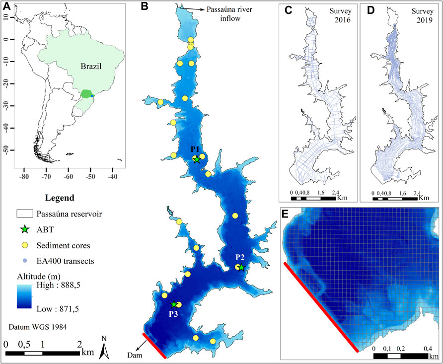
FIGURE 1. (A) Location of the study site Passaúna Reservoir in South America; (B) Bathymetric map of Passaúna Reservoir and measurement locations (see legend); (C) echo-sounding transects during the survey in 2016; (D) echo-sounding transects during the 2019 survey; (E) Zoom to the dam area with overlaid analysis grid.

According to the updated Köppen climate classification, the region is characterized by temperate oceanic climate (Cfb), with monthly mean temperatures below 22°C for all months and no significant precipitation difference between seasons (Beck et al., 2018). The mean annual precipitation in the region ranges between 1,400 and 1,600 mm. During measurements covering a full annual cycle conducted in 2018–2019, the reservoir water temperature ranged from 16 to 28°C, with August being the coldest month with an averaged bottom temperature of 16.5°C (Ishikawa et al., 2021). Meteorological data for this study was provided by the company SANEPAR which manages the reservoir. Weather data is logged at a station installed near to the dam.

2.2 Ebullition Flux and Pore Water Methane Concentration Measurements

Ebullition flux and pore water methane concentration were measured at three sampling sites distributed along the reservoir (Figure 1B). The site P1 is located most closely to the main river inflow (Passaúna River) at a water depth of 8 m. The site P2 was placed in the central region of the reservoir, near to the water intake facility, where the water depth is 12.5 m. Site P3, was placed in the deepest region of the reservoir, approximately 810 m upstream of the dam, at a water depth of 14 m.

The ebullition measurements analyzed in the present study are a continuation of the measurements that started in 2017 and were described by Marcon et al. (2019). The ebullition flux was monitored continuously by automated bubble traps (ABT, Senect GmbH, Germany) from January to March 2019. The ABT were attached to a surface buoy and deployed at a depth of approximately 4–5 m above the sediment surface. The device consists of a 1 m diameter funnel, which collects rising gas bubbles, and a differential pressure sensor to monitor the gas volume that accumulated during fixed time intervals (30 s). The device also measured water temperature and pressure, which were used to convert the collected gas volume to standard pressure and temperature (1,013.25 mbar and 20°C). In addition, bubbles were collected from the sediment near to the ABT’s location to estimate the methane fraction within the bubbles. The captured gas was transferred to vials with saturated salt solution until its analysis in the laboratory with an Ultraportable Greenhouse Gas Analyzer (UGGA, Los Gatos Research Inc.).

Dissolved methane concentration in the sediment pore water was measured with a dialysis pore water sampler (DPS) as described by Hilgert (2014) and Hölzlwimmer (2013). The DPS is a perforated aluminum frame of 70 cm height divided into 15 chambers of 4 cm width each. A cellulose membrane bag of 50 ml filled with ultra-pure water was added to each chamber. On 02 February 2019 three DPS’s were deployed by divers in the bottom sediment at each ABT location (P1, P2, and P3) and positioned vertically such that seven chambers were inside the sediment and eight chambers in the overlaying water column. The devices were deployed for 5 days, to allow the ultra-pure water of the bags to equilibrate with the ambient water or pore water. Directly after recovery, a sample of 5 ml was extracted from each bag with a plastic syringe, a headspace of 5 ml was created in the syringe and after rigorous shaking, the headspace gas was transferred to vials containing saturated salt solution, previously sealed with a rubber stopper and crimp-capped. The vials were stored upside-down until analysis in the laboratory, where the methane concentration was measured with an Ultraportable Greenhouse Gas Analyzer (UGGA, Los Gatos Research Inc.) in a closed loop arrangement, as described by Wilkinson et al. (2018); Wilkinson et al. (2019b). The corresponding methane concentration in the water sample ($C_{CH4}$ in mol L⁻¹) was calculated as proposed by Bossard et al. (1981) as:

$C_{CH4}=\left(\frac{V_{Hs}}{V_W}\frac{\left(X_{eq}-X_{back}\right)}{RT}+X_{eq}{K}_H\right)\times P_{atm} ,$

where $V_{Hs}$ is the headspace volume in L, $V_W$ is the water sample volume in L, $X_{eq}$ and $X_{back}$ are the methane mole fractions measured with the gas analyzer after equilibration and in the initial headspace in ppm respectively. $K_H$ is the temperature dependent Henry gas solubility coefficient, which was calculated according to Goldenfum (2010) in mol L⁻¹ atm⁻¹, $T$ is temperature in K, $R$ is the gas constant ($R$ = 0.08205 L atm mol⁻¹ K⁻¹), and $P_{atm}$ is the atmospheric pressure in atm.

2.3 Data Re-Analyses

The following sections describe the re-analysis and additional processing of data from acoustic surveys conducted in Passaúna Reservoir during former studies.

2.3.1 Potential Methane Production

The potential methane production (PMP) in sediment samples collected at the ABT deployment locations (P1, P2, and P3, Figure 1) was analyzed in Hilgert et al. (2019b). The potential production rates were obtained for samples from different sediment layers, that were anaerobically incubated under laboratory conditions as described by Wilkinson et al. (2015). The potential methane production was calculated for in-situ sediment temperature by the relationship proposed by Wilkinson et al. (2019a)

$PM{P}_T=PM{P}_{20} {10}^{\theta \left(T-20\right)},$

where $PM{P}_T$ (in mgCH₄ L⁻¹ d⁻¹) is the potential methane production rate at in-situ temperature $T$ (in °C), and $PM{P}_{20}$ is the rate measured during laboratorial incubations at 20°C. We used a value of the temperature coefficient $\theta$ of 0.045, as suggested by Wilkinson et al. (2019a) for incubated freshwater sediments.

The PMP was integrated over the top 10 cm sediment layer by multiplication of the averaged PMP_T with layer thickness to provide a potential areal flux (in mgCH₄ m⁻² d⁻¹) at the sediment water interface (Wilkinson et al., 2019a).

2.3.2 Acoustic Parameters and Mapping of Gas Content in the Sediment

The analysis of gas content in the sediment conducted in the present study is based on echo-sounding surveys with a dual frequency (38 and 200 kHz) echo-sounder EA400 (Kongsberg Inc. 2006). The surveys have been analyzed for different aspects before (Sotiri et al., 2019a; 2019b, 2021). For the measurements, the echo-sounder was fixed 0.45 m below the water surface to an aluminum vessel, and zig-zag transects were measured along and across the reservoir (Figure 1 panels (C) and (D)). The surveys were conducted from 26 February to 07 March 2016, and from 04 February to 07 February 2019 and covered approximate distances of 75 km in 2016 and 219 km in 2019. The echo-sounder was operated with an output power of 100 W, and pulse lengths of 0.512 and 0.128 ms for the 38 and 200 kHz channels, respectively, resulting in vertical resolutions of 0.096 and 0.024 m for the two frequencies. For an average water depth of 8.3 m, the footprint area of the acoustic beams were 5.0 m² (38 kHz with opening angles of 13° for the longitudinal and 21° for the transversal direction) and 0.8 m² (200 kHz with longitudinal and transversal opening angle of 7°). The measurement positions during the surveys were recorded using a Leica 1200 DGPS (Differential Global Positioning System) system. Vertical temperature profiles for sound speed correction were measured with a CTD–Conductivity-Temperature-Depth (CastAway®-CTD) probe.

For this study, the conversion and processing of the acoustic data was done using the Sonar5-Pro software (Lindem Data Acquisition, Oslo, Norway). Two main acoustic parameters of the first bottom echo from the 200 kHz measurements exported from the software were considered: attack and maximum backscatter strength. The values are defined for each ping (sound pulse). The envelope of the backscatter profile across the sediment-water interface is generally characterized by an increase of the backscatter strength at the sediment surface, reaching a peak amplitude (maximum backscatter), and followed by a decay with increasing depth (Sternlicht and de Moustier, 2003) (see Supplementary Figure S1). Attack is defined as the vertically integrated backscatter strength values occurring over a duration of one pulse length from the bottom detection point (Hilgert et al., 2016) and was used to estimate the organic content in the sediment (see below). The maximum backscatter (named as bottom peak in Sonar5-Pro), is the maximum value (dB) of the backscatter that occurred starting from the detected bottom downward and searched by the software until three transmitted pulse lengths (Balk et al., 2011).

Anderson and Martinez (2015) analyzed the acoustic parameters from three productive lakes in Southern California (United States). The authors established a relationship between maximum backscatter (measurements at 201 kHz frequency) and gas volume in the sediment (corrected to the local hydrostatic pressure) per unit area:

$gc= e^{\left(0.327\times S_{y max}+3.48\right)},$

where $gc$ is gas content per unit area in L m⁻² and $S_{y max}$ is the maximum backscatter strength in dB. The maximum backscatter was found to explain 93% of the variance in estimated gas content (R² = 0.93) (Anderson and Martinez, 2015). We adopted the proposed equation to estimate the gas content per unit area, hereinafter also referred to as gas content, in the sediment of Passaúna Reservoir, which is justified by the similar conditions in respect to water depths, trophic state, bottom sediments, and acoustic measurements in comparison to the study of Anderson and Martinez (2015) (Table 1). Although the pulse lengths differed between the studies, the maximum backscatter values are expected to be unaffected, and thus the application of Anderson and Martinez (2015) relationship is expected to be a valid estimate for addressing the spatial variability of sediment gas content in Passaúna Reservoir during both echo-sounding surveys (2016 and 2019). The gas content estimated for the higher-resolution survey conducted in 2019 was then analyzed in relation to organic matter content in the sediment (LOI at 550°C), sediment magnitude distribution, and bathymetry.

TABLE 1

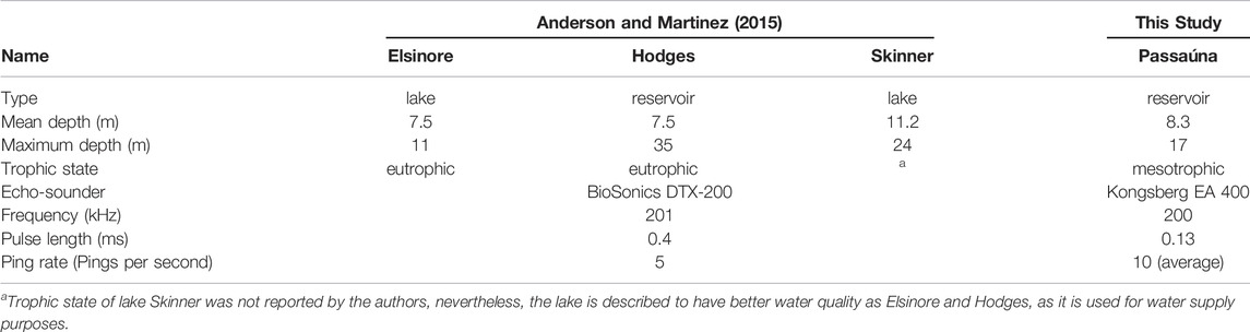
TABLE 1. Summary of the study site characteristics and echo-sounder details of the study by Anderson and Martinez (2015) for which an empirical relationship between maximum backscatter strength and sediment gas content was established, and the corresponding information for Passaúna Reservoir.

2.3.3 Organic Matter, Sediment Thickness, and Bathymetry

Information on the reservoir bathymetry, organic matter content in sediments, and sediment thickness distribution were taken from Sotiri et al. (2021). The reservoir bathymetry was measured with a multibeam echo sounder (WASSP F3Xi) measuring with a frequency of 160 kHz. The bathymetric map was then used in this study to derive the bottom slope.

Sediment distribution and magnitude in the reservoir was measured by Sotiri et al. (2021) with a dynamic free-fall penetrometer. The mapping of the organic matter content was derived from a former study conducted by Sotiri (2020) at Passaúna Reservoir, which was based on measurements of loss on ignition at 550°C (LOI 550°C) for more than 20 sediment cores with echo-sounding measurements at each core location. The empirical relationship proposed by Sotiri (2020) had a R² of 0.66, in which LOI is calculated from a polynomial equation as a function of the acoustic parameter Attack ($Att$),

$LOI 550°C= -44.6+\left(-10.4 Att\right)+\left(-0.6At{t}^2\right)+\left(-0.01At{t}^3\right),$

where $Att$ is derived from the echo-sounder EA400 measurements at 200 kHz frequency.

The LOI is widely applied as a proxy for quantifying organic matter content in the sediment, nevertheless for clay rich sediments LOI is reported to overestimate the organic matter content, as during the burning at 550°C the loss of clay structural water and breakdown of carbonates have a share on the weight loss in addition to the organic matter (Frangipane et al., 2008). Therefore, although LOI is adopted as a proxy for organic matter distribution, its absolute values might differ from organic matter measured by other methods. However, for sediment samples from two reservoirs in a neighboring watershed, Hilgert (2014) found strong significant correlation (Pearson correlation 0.76) between LOI and organic carbon, which showed the potential to consider LOI for representing organic matter distribution as the organic carbon was not directly measured at Passaúna reservoir.

2.4 Statistical Models for Predicting the Sediment Gas Content

We developed statistical and data driven models to predict the spatial distribution of the estimated sediment gas content from maps of water depth, sediment thickness, and organic matter content (LOI 550°C) as predictor variables. The input variables and the prediction of gas content were analyzed within a spatial grid created for the reservoir based on the acoustic survey conducted in 2019. The analysis grid was created using the Geographical Information System (GIS) software ArcGIS (v. 10.2.2) with the geoprocessing tool Fishnet, in which we divided the surface area of Passaúna reservoir in 8,454 rectangular grid cells with dimensions of 33 m by 33 m (Figure 1E). Additional information about the grid selection is provided in the supplementary material (Supplementary Figure S2). The size of the grid cells was chosen to be sufficiently small to resolve the spatial heterogeneities of the measured parameters occurring in the sediment (longitudinal and transversal variations), and large enough to analyze all parameters in terms of spatial averages, that integrate small-scale (unresolved) structures. Mean values of all parameters (water depth, bottom slope, sediment thickness, organic content through LOI 550°C, and gas content) were calculated for all grid cells for which survey data are available.

To reduce the uncertainty of parameters derived from acoustic measurements, we excluded grid cells with an average bottom slope larger than 10° from all subsequent analysis. This is justified by the fact that the acoustic backscatter strength of sediment surfaces and sediment layers depends on the grazing angle of the soundwave (angle between incident wave and the tangent to the surface). For incidence angles of the soundwave near to the normal direction in relation to the sediment surface, scattering (attack values) dominate the backscattering, in contrast for inclined conditions (i.e., grazing angles in the range 30–60°) the volume scattering dominates (Fonseca et al., 2002). Sternlicht and de Moustier (2003) showed that the effect of slopes is lengthening the echo, resulting in prolongated rising and decaying parts of the echograms, leading to a reduction of the maximum backscatter independent from the sediment composition.

Steep slopes in Passaúna Reservoir occurred mainly near the banks or along the old Thalweg of the Passaúna River as described by Sotiri et al. (2021). The slope threshold resulted in removal of 1,034 grid cells, thus 4,651 grid cells were classified as valid cells (with data of all parameters measured and in agreement with the slope criterion).

The potential CH₄ production (PMP), dissolved CH₄ concentration in pore water, and ebullition were not extrapolated to the entire reservoir, as they were measured at only three locations. Nevertheless, the measurements are used to support our discussion on the spatial distribution and dynamics of the estimated sediment gas content.

Three multiple linear regression models were tested for gas content prediction in which the water depth, sediment thickness, and LOI 550°C were the predictors. The first model (MLR I) was a simple multiple linear regression, for the second model (MLR II) the predicted value (gas content) was log transformed, and for the third statistical model a stepwise multiple regression (SMR) with untransformed values was performed. The main difference of the stepwise multiple regression to the two other models is that predictors are included sequentially in the model and accepted if a p-value criterion is met for a significance level of 5%. Furthermore, interactions of the input variables are tested in this model as predictors.

The data driven model is a supervised artificial neural network (ANN). The ANN architecture had three layers, one input layer with three neurons, one hidden layer with 10 neurons, and one output layer with one neuron (Figure 2). The input variables were water depth, sediment thickness, and LOI 550°C. For improving the performance of the ANN, the input variables were normalized to range from 0 to 1. The Hidden layer is a processing layer where the transfer function was a hyperbolic tangent sigmoid function, in which the values transferred to the output layer will vary between $-$ 1 to 1. The output layer is the gas content per unit area in L m⁻².

FIGURE 2

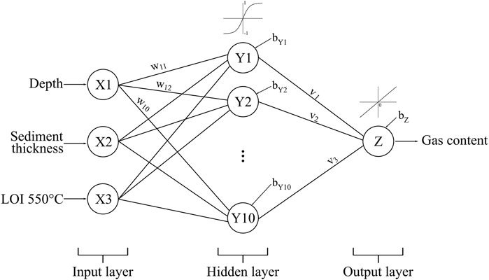
FIGURE 2. Architecture of the artificial neural network implemented in this study for the prediction of gas content in sediment. X1, X2, and X3 are the neurons in the input layer, Y1 to Y10 are the neurons in the hidden, Z is the neuron at the output layer. w denotes the weight of each neuron connection from the input to the hidden layer, v are the weights of hidden layer connections to the output layer, and b are the bias for each neuron in the hidden and output layers.

We used the Levenberg—Marquardt backpropagation for training of the ANN. During the training step, the algorithm randomly divided the data into three parts. 70% of the data points are used for the actual training of the neural network, 15% are used for the validation of the ANN during the training calculations to avoid overfitting, and the remaining 15% are not included for the training and are used for testing the trained model.

The model’s result for gas content prediction were evaluated considering the coefficient of determination (R²) between observed and predicted gas content and through the relative error. The relative error, which was expressed in percentage, was calculated for each grid cell as

$Erro{r}_{relative}= \left(\frac{\left|y_{predicted}-y_{observed}\right|}{y_{observed}}\right)\times 100$

where $y_{predicted}$ and $y_{observed}$ are the predicted and estimated gas content, respectively.

Lastly, the gas content in the sediment derived from the hydro acoustic surveys performed in 2016 and in 2019 was compared to analyze the temporal changes in different regions of the reservoir and to check the application of the prediction model from 2019 against the measurements of 2016. The temporal change in gas content between 2016 and 2019 was tested for each valid grid cell using a non-parametric hypothesis test (Wilcoxon rank sum test), considering only cells that contained 30 or more pings (sound pulses), which resulted in 1,321 cells for the comparison.

3 Results

3.1 PMP, Porewater CH₄, and Ebullition Gas Flux

The highest values of potential methane production for all three sampling locations were found in the top 10 cm sediment layer. The maximum PMP values ranged from 3.4 mgCH₄ L⁻¹ d⁻¹ at P3 to 5.9 mgCH₄ L⁻¹ d⁻¹ at P2. From the near-surface layer, PMP decayed approximately exponentially with increasing depth in the sediment (Figure 3A). The integrated temperature corrected PMP for the top 10 cm resulted in a potential methane flux at the water-sediment interface of 306.4, 450.2, and 91.1 mgCH₄ m⁻² d⁻¹ at locations P1, P2, and P3 respectively.

FIGURE 3

FIGURE 3. (A) Depth profiles of potential methane production (PMP) in the sediment [data from Hilgert et al. (2019b)] (B) dissolved methane concentration in the pore water and overlaying water at the sediment-water interface measured in 2019. The origin of the depth-axis is at the water-sediment interface. The dashed lines show the respective CH₄ solubility limit for each location, calculated as a function of temperature, salinity, and hydrostatic pressure according to Dale et al. (2008). (C) Time series of accumulated gas volume recorded by the automated bubble traps (ABTs) from 1 January to 15 February 2019. The grey shaded area marks the days when the echo-sounding survey was conducted in 2019. All three panels show measurements at the three sampling locations in Passaúna Reservoir (P1, P2 and P3, see Figure 1).

Dissolved methane concentration was lowest in the overlying water with a strong increase in concentration towards the water-sediment interface (Figure 3B). In the sediment, the dissolved methane concentration continued to increase with increasing depth with comparable vertical gradients at all three locations. The maximum porewater methane concentrations were measured in the deepest DPS chamber at 25–30 cm sediment depth (1.4 mmol L⁻¹ at location P1, 1.3 mmol L⁻¹ at P2, and 1.2 mmol L⁻¹ at P3).

Gas ebullition flux was continuously measured during 45 days, starting prior to the acoustic survey conducted in 2019. The largest amount of gas was collected by the bubble trap at location P1 (9.3 L), followed by locations P2 (6.0 L), and P3 (3.7 L) (Figure 3C). For the 45 measurement days, the recorded volume represents a methane ebullition flux of 118.1, 77.5, and 48.1 mgCH₄ m⁻² d⁻¹ at the locations P1, P2, and P3 respectively (with CH₄ fraction in bubbles collected from the three locations of 68.9 ± 6.8%).

At locations P2 and P3 (near to the water intake and in the dam region) the dynamics of gas accumulation is characterized by stepwise increases, in which periods of several days without ebullition are interrupted by ebullition events. At P1 in contrast, more continuous ebullition events occurred throughout the measurement period, as it can be observed by the prolonged rise of the accumulated gas volume curve (Figure 3C). At all locations, pronounced ebullition was observed on February 5th during the period when the echo-sounding surveys were conducted. This ebullition event was associated with a weather change; from February 04th to February 07th, there was a reduction of the air temperature by approximately 10°C in comparison to the previous days (Supplementary Figure S3). Atmospheric pressure strongly decreased starting from February 05th. During the surveys, the water level in the reservoir decreased by 2 cm (from February 05th to February 07th) and the mean wind velocity was 1.6 ± 0.4 m s⁻¹ (average ± standard deviation).

3.2 Acoustic Mapping of the Reservoir Sediment

According to Sotiri et al. (2021), the reservoir bottom is overlaid by an unconsolidated fine-grained low-density material layer. The analysis of the sediment cores showed that the bottom sediment is dominated by silt-clay grain sizes and an average loss on ignition (LOI) of 17 ± 8.5%. The averaged LOI in the sediment estimated from the acoustic parameter attack (Figure 4C) was 14.7 ± 4.9% for the whole reservoir, in which 3.9% of the valid grid cells had LOI of less than 10% and a minimum value of 1.8%.

FIGURE 4

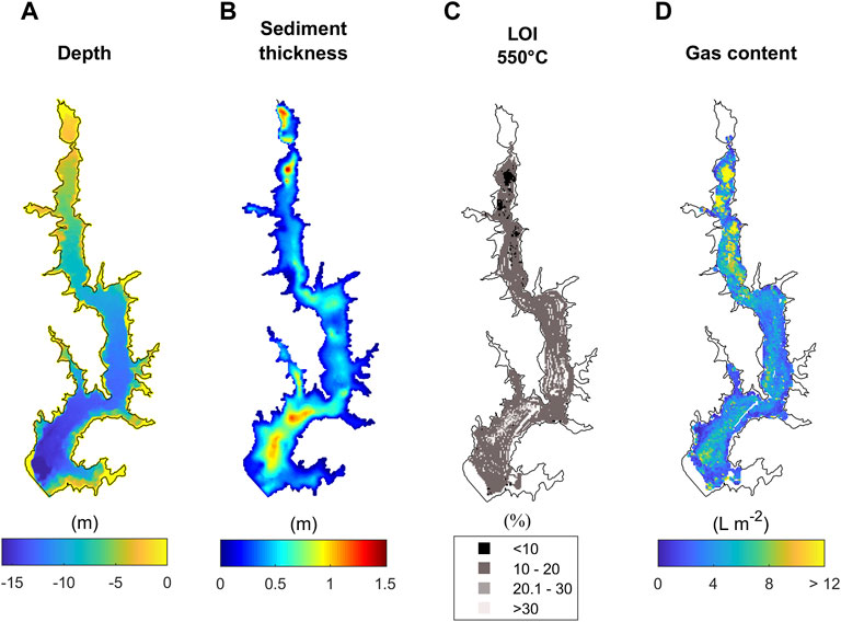
FIGURE 4. (A) Passaúna Reservoir water depth and (B) sediment thickness distribution from Sotiri et al. (2021). (C) LOI 550°C extrapolated to the entire reservoir as a function of the acoustic parameter Attack with the relation proposed by Sotiri (2020). (D) Distribution of estimated gas content in the sediment estimated from the equation proposed by Anderson and Martinez (2015). All data are averaged for individual cells of the analysis grid. Blank areas in (C) and (D) indicate missing data and grid cells with high bottom slope (>10°).

The sediment magnitude estimated by Sotiri et al. (2021) varied from 0 to a maximum of 1.8 m, with highest sediment accumulation in the upstream region near to the river inflow and in the region near to the dam (see Figure 4B), where the water depth varies from 10 to 15 m. Average sediment thickness in the analysis grid ranged from 0 to 1.5 m, with a mean value of 0.5 ± 0.2 m.

The overall mean value of the maximum acoustic backscatter in the analyzed grid cells was −6.6 ± 2.0 dB. According to the empirical relationship proposed by Anderson and Martinez (2015), this corresponds to a mean sediment gas content for the whole reservoir of 4.6 ± 3.2 L m⁻². The largest values of sediment gas content were estimated for the upstream region of the reservoir, whilst the smallest values were found near the banks and in the deepest region of the reservoir in front of the dam (Figure 4D). Elevated (above average) gas content was also estimated for the central part of the deeper region near the dam. At the locations where the automated bubble traps were deployed, the averaged gas content in the sediment was 6.2 ± 2.1 L m⁻², 4.1 ± 1.6 L m⁻², and 5.6 ± 2.0 L m⁻², for the P1 to P3 respectively (Table 2).

TABLE 2

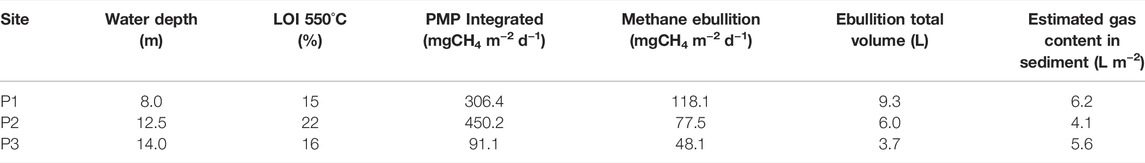
TABLE 2. Parameters at the three monitoring sites P1, P2, and P3. Loss on ignition (LOI) from sediment cores were provided by Sotiri (2020); the PMP was integrated for the top 10 cm sediment layer; methane ebullition was calculated with the measured methane fraction in the gas bubbles of 68.9%; and the estimated gas content in the sediment was acoustically derived and averaged for the areas surrounding the location of each bubble trap deployment.

3.3 Models for the Prediction of Gas Content in the Sediment

The variables water depth, which ranged from 1.4–15.35 m (8.9 ± 3.3 m), sediment thickness with values in the range of 0.03–1.5 m (0.5 ± 0.2 m), and LOI 550°C varying from 1.8–53.5% (14.7 ± 4.9%) were tested as predictor variables for the gas content in the sediment, which varied from 0.1 to 40.4 L m⁻² (4.6 ± 3.2 L m⁻²). In an exploratory analysis of the variables, a Spearman rank correlation test was applied to check statistical correlation among the parameters (see Supplementary Figure S4). Considering the individual correlations between gas content and the predictor variables, the strongest correlation was found between gas content and LOI (Spearman correlation $r_s=-0.58$ and p = 0), whereas weaker, yet significant, correlations were found between gas content and water depth ($r_s=-0.12$, p < $0.05$) and gas content and sediment thickness ( $r_s=-0.18$ p < $0.05$).

Multiple linear regression (model MLR I) resulted in a coefficient of determination (R²) of estimated gas content of 0.24 (p < $0.05$for the F-test on the model). As the distribution of gas content in the sediment deviates from a normal distribution (Supplementary Figure S4), a multiple linear regression with log transformed gas content (MLR II) was tested, resulting in a R² of 0.16 (p < $0.05$for the F-test on the model). The stepwise multiple regression (SMR) resulted in a R² of 0.54 (p = 0 for the F-test on the model). The full model equations are presented in Table 3. The trained artificial neural network (ANN) reproduced 89% of the gas content variance (R² = 0.89 for all data points). Comparable coefficients of determination were obtained for the test data set which was not included during the training of the ANN (R² = 0.91, Supplementary Figure S5).

TABLE 3

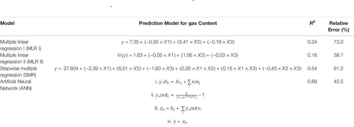
TABLE 3. Summary of the three statistical models (MLR I, MLR II, and SMR) and the data driven model (ANN) tested for the prediction of sediment gas content ($\mathit{y}$) from the variables $\mathit{X}1$ = water depth, $\mathit{X}2$ = sediment thickness, and $\mathit{X}3$ = LOI at 550°C. For the trained ANN $\mathit{y}\_\mathit{i}{\mathit{n}}_{\mathit{k}}$ denotes the input value for neuron ${\mathit{Y}}_{\mathit{k}}$, ${\mathit{b}}_{{\mathit{Y}}_{\mathit{k}}}$ is the bias of neuron ${\mathit{Y}}_{\mathit{k}}$ of the hidden layer, and ${\mathit{x}}_{\mathit{i}}$ is the value of the predictor $\mathit{i}$. $\mathit{y}\_\mathit{ou}{\mathit{t}}_{\mathit{k}}$ is the value calculated by the transfer function and ${\mathit{b}}_{\mathit{z}}$ is the bias of the output neuron. ${\mathit{w}}_{\mathit{ij}}$, and ${\mathit{v}}_{\mathit{i}}$ are the weights of the neurons connecting the input to the hidden layer and the hidden layer to the output neuron, respectively.

The largest relative errors (>80%) for all models occurred near the banks at deepest region near to the dam (Figure 5 panels (B), (C), and (D)). The averaged relative error for the 4,651 grid cells was 42.5, 61.2, and 72.96% for the ANN, SMR, and MLR I model, respectively. In addition, the linear regressions applied to the predicted and estimated gas content indicate a systematic underestimation of all three models compared to observations (Figure 5A). The frequency distributions of the relative error showed that for all models the most frequent relative errors obtained were smaller than 25% (see Supplementary Figure S6 panels (A) and (B)). On the other hand, the largest relative errors values (above 500%) occurred for the grid cells with gas content per unit area of less than 4 L m⁻².

FIGURE 5

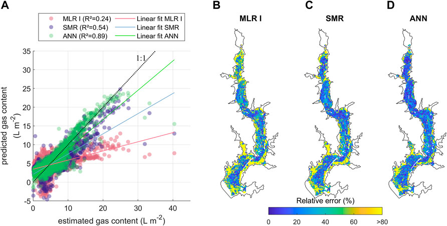
FIGURE 5. (A) Scatter plot of predicted vs. estimated gas content and gas content for the survey in 2019 using three different empirical models (model MLR I are pink dots, SMR are the purple dots, and ANN are the green dots). Colored solid lines show linear regressions for each model with the following regression equations: MLR I $\mathit{y}=3.46+0.24\mathit{x}$ (pink line); SMR $\mathit{y}=2.11+0.54\mathit{x}$ (blue line), and ANN $\mathit{y}=1.02+0.78\mathit{x}$ (green line). The dotted black line shows a 1:1 ($\mathit{y}=\mathit{x}$) relationship. (B) Spatial distribution of the relative error between predicted and estimated gas content from the multiple linear regression I (MLR I) in which 21.6% of the grid cells had errors larger than 80%. (C) Relative error of the predicted gas content from the stepwise multiple regression (SMR) in which 17.7% of the grid cells had errors larger than 80%. (D) relative error of the gas content predicted by the artificial neural network (ANN) in which 10.7% of the grid cells had error larger than 80%.

3.4 Temporal Variability of Gas Distribution in the Sediment

The gas content in the sediment was also calculated with the hydro acoustic data recorded during the 2016 survey. In both surveys (March 2016 and February 2019), the water column was thermally stratified, with a warmer top layer of ∼26°C and colder bottom water with the lowest temperature of ∼21°C at location P3 (Supplementary Figure S7 panels (A) to (C)). Small variations of the reservoir water level were recorded during the hydro acoustic surveys of both years (3 cm in 2016 and 2 cm in 2019). However, for the 2016 survey the water level was ∼1 m higher than the water level recorded during the survey of 2019.

In both years, the estimated gas content in the sediment of the reservoir was similar with mean values of 4.4 ± 3.1 L m⁻² in 2016 and 4.6 ± 3.2 L m⁻² in 2019. Nevertheless, the range of the spatial variation of the gas content was slightly different with larger values in 2016 (2016: 0.1–57.0 L m⁻²; 2019: 0.1–40.4 L m⁻²). In both years, the largest gas content was estimated for sediments in the upstream part of the reservoir. Nevertheless, the coarser spatial resolution of the echo-sounding transects conducted in 2016 (partial loss of data) did not allow for capturing the spatial structure of the gas content hotspots in this region (Figure 6A).

FIGURE 6

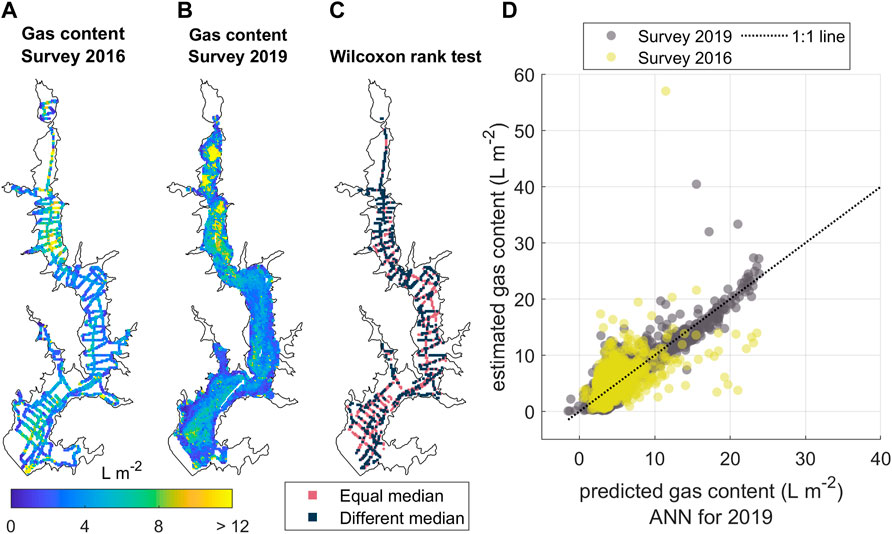
FIGURE 6. (A) Areal gas content in the sediment for the 2016 acoustic survey. (B) Gas content in the sediment for the 2019 survey. (C) Results of the Wilcoxon rank test comparing the median gas content from both years, in which pink dots mark grid cells for which the null hypothesis of data from both years having the same distribution and equal median is accepted, and the dark blue dots mark the grid cells where the null hypothesis was rejected. (D) Scatter plot of observed vs. predicted gas content by the artificial neural network model with data from 2016 (yellow dots) and 2019 (grey dots). The dotted black line shows a 1:1 relationship.

As the spatial coverage of the acoustic transects during the 2016 survey was coarser than in the 2019 measurements, only 1,321 grid cells could be considered for comparing the gas content between both years. A non-parametric hypothesis test was performed for each grid cell to verify the occurrence of a significant difference in the median gas content between both years (Figure 6). 48% of the cells had no significant difference in the median gas content and 52% were found to have different median gas content. Significant differences between both years occurred mainly at the shallower upstream part of the reservoir (near monitoring location P1), where the gas content was lower in 2019 compared to 2016 (Supplementary Figure S8). Higher gas content was detected in the reservoir stretch between the monitoring locations P1 and P3.

Lastly, we compared the predicted gas content from the artificial neural network model, which was based on 2019 data, with estimated gas content in 2016 and 2019. The gas content in the sediment in 2016 agreed with the predicted and estimated gas content of 2019, as shown in Figure 6D (R² = 0.45 for a linear fit with no intercept between predicted gas content from the ANN model and estimated gas content in 2016, p = 0 for the estimated coefficient). As previously mentioned, the upstream areas of potential high gas content in the sediment were not resolved in the 2016 survey. Nevertheless, grid cells with higher gas content in 2016 were observed in the vicinity of that region.

4 Discussion

4.1 Spatial-Temporal Mapping of Sediment Gas Content

A high spatial resolution sediment gas content mapping was obtained as a function of the acoustic parameter maximum backscatter using the empirical relationship proposed by (Anderson and Martinez, 2015). The average maximum backscatter in Passaúna Reservoir ($-$6.6 ± 2.0 dB) is in the range of the values obtained by Anderson and Martinez (2015) for the eutrophic reservoir Hodges. The gas content ranged between 0.1 and 40.4 L m⁻², which for a 10 cm sediment layer represents a volumetric gas content of 0.1–40.4% (vol). The addition of gas voids to the sediment matrix results in a decrease in the sediment wet bulk density leading to instability of the sediment matrix and release of gas bubbles (Van Kessel and Van Kesteren, 2002; Liu et al., 2018). Van Kessel and Van Kesteren (2002) found that for muddy sediments, gas fraction in the range of 25–37% results in instabilities in the sediment matrix. For Passaúna reservoir less then 1% of the cells had gas content larger than 25% (Supplementary Figure S9). Moreover, considering the sediment wet bulk density mapped by Sotiri et al. (2019b), the regions with lower wet bulk density had relatively less gas content.

For lake Kinneret the upper limit of gas fraction in the sediment from acoustic measurements were 0.2% (Katsnelson et al., 2017) and 3.8% (Uzhansky et al., 2020). Nevertheless, for laboratory conditions Liu et al. (2016) found a maximum gas content in incubated clay sediment of 46.8% with a depth-average of 18.8% for this fine sediment. Thus, the few highest fractions of gas content found (<1% cells) at Passaúna are in the same range as the values reported by Liu et al. (2016), whereas the averaged values of gas content are one order the values found in Lake Kinneret (Uzhansky et al., 2020).

Transversal and longitudinal variation of gas content in the sediment were observed along the reservoir. Longitudinally, the largest amount of free gas in the sediment was detected in the upstream part of the reservoir, closest to the main inflow (Figure 4D), in a region with the largest sediment thickness and low water depth. We found that the gas content in the sediment tended to be higher in regions of preferred sedimentation (i.e. large sediment thickness), nevertheless with gas content magnitude being additionally affected by the water depth. For instance, at the deepest region of the reservoir where elevated sediment deposition was also mapped, the gas content was lower (up to 10 L m⁻²) compared to the shallow upstream region (up to 30 L m⁻², Supplementary Figure S10C).

The occurrence of temporal change in gas content in the sediment was verified by analyzing two available echo-sounding surveys conducted 3 years apart from each other. The two surveys were done during summer at comparable water temperature and thermal stratification, and with small water level variation during both surveys, see Supplementary Figure S7. The mean sediment gas content was similar during both surveys (4.4 ± 3.1 L m⁻² in 2016 and 4.6 ± 3.2 L m⁻² in 2019). The range of its spatial variability, however, differed and the maximum gas content in 2016 (56.9 L m⁻²) was almost 50% higher than the maximum value in 2019 (40.4 L m⁻²). We found that 52% of the analyzed sediment area had statistically different gas content between both surveys and lower gas content in 2019 was mainly estimated for the shallower upstream region (around location P1) (see Supplementary Figure S8). The lower gas content can be related to the 1 m higher water level in 2016. Higher water level would represent additional hydrostatic pressure at the water-sediment interface, and thus increases the burden for bubble formation. A strong linear decrease of sediment gas content with increasing water level has been observed in Lake Kinneret, where acoustic surveys were conducted across several years (Uzhansky et al., 2020). In addition to water depth, the proximity to the main inflow Passaúna river makes this region more affected by floods events which can alter the bottom sediment conditions.

Although small-scale variability of gas content in the sediment is not resolved in this study, either due to the echo response which is resulting from a bottom area (0.8 m² at 8.3 m depth) and from the averaging with the grid cell; measurements with closer distributed hydro acoustic transects were important for detecting spatial patterns in the gas content. For instance, in the 2016 survey, which covered a distance 3 times shorter than the survey performed in 2019, the areas of high gas content located at the upstream region of the reservoir were not captured due to missing data points.

4.2 Methane Production, Concentration, and Ebullition

The results from the incubated sediment cores showed that the top sediment layer has the largest potential for methane production (PMP). The finding that the top 10 cm sediment layer is most productive is in agreement with Isidorova et al. (2019), who considered sediment within the range of sediment age (<6–12 years) as still active for methane production. In Passaúna, the first 10 cm of sediment have an age of 5 years, based on the findings of Sotiri et al. (2021), who estimated a sedimentation rate of 1.9 cm yr⁻¹.

The integrated PMP over the 10 cm depth resulted in a potential methane flux at the sediment water interface of 306, 450, and 91 mgCH₄ m⁻² d⁻¹ at the locations P1, P2, and P3 respectively at an average sediment temperature. The PMP of Passaúna sediment is within the range found in sediments from impoundments in Germany (Wilkinson et al., 2015) and the potential fluxes at the water-sediment interface are higher than the values reported for tropical lakes in Uganda (15.4–144 mgCH₄ m⁻² d⁻¹) (Morana et al., 2020). The largest integrated PMP value at location P2 coincided with the highest organic matter content (indicated by LOI 550°C) from sediment cores (LOI 550°C 15% at P1, 22% at P2, and 16% at P3), which is in agreement with other studies that reported enhanced methane production for sediments with higher organic matter content (West et al., 2012; Grasset et al., 2021).

The averaged methane ebullition fluxes were 2.6, 5.8, and 1.9 times smaller than the corresponding potential flux at the water-sediment interface estimated from the integrated PMP at the three locations (see Table 2). The lower emission rates compared to sediment CH₄ production differ from observations by Wilkinson et al. (2015), in which the measured ebullition flux was comparable to the potential methane flux from PMP of shallow (<4 m) impoundments. We attribute this difference to the higher water depths of Passaúna Reservoir (average of 8.3 m), which can favour the diffusive flux of methane from the sediment (Langenegger et al., 2019). The transported methane can accumulate in the overlaying water where it is susceptible to oxidation or release to the atmosphere during mixing events (Vachon et al., 2019). In fact, from the dissolved methane concentrations in the water overlaying the sediment, the shallowest upstream location, which is more likely to have mixing due to its lower water depth, had methane concentrations that were one order of magnitude smaller than at the other two sites (0.02, 0.36, and 0.33 mmolCH₄ L⁻¹ for locations P1, P2, and P3).

Furthermore, although location P1 had a lower integrated PMP than location P2, the methane ebullition flux was 1.5 times higher, which we attribute in addition to the enhanced diffusion of CH₄ to the water, to the larger water depth and thus, to the total pressure at the water-sediment interface. As the solubility limit of methane in the porewater increases with higher hydrostatic pressure (Figure 3B), larger dissolved gas concentrations are required for gas bubble formation (Bazhin, 2003; Langenegger et al., 2019). As shown in Figure 1, the methane concentration measured in sediment porewater at locations P2 and P3 were lower than the methane saturation limit considering the local water depth at these two sites. On the other hand, at the shallower location P1, the methane concentration in the sediment porewater was above the saturation limit for the deeper sediment layers. Lastly, an important aspect to consider, is that the PMP was obtained for laboratory conditions which may differ from the dynamic environmental conditions in the reservoir.

Ebullition is widely characterized in the literature as being highly variable in space and in time (Wik et al., 2013; Maeck et al., 2014). For Passaúna Reservoir, it was previously observed that ebullition events at the three monitoring locations where synchronized on a daily basis in which the ebullition events were triggered by large-scale forcing, such as drops in the atmospheric pressure (Marcon et al., 2019). For the 45-days time-series analyzed in the present study, a larger release of gas from the sediment was observed for February 4th to February 7th, which we could associate with the beginning of a period of decreasing atmospheric pressure (Supplementary Figure S3). We suggest that the drop in atmospheric pressure during the echo-sounding survey in 2019 potentially triggered gas release from the bottom sediment. Nevertheless, considering the elevated potential methane production of the bottom sediments, we assumed that the spatial patterns of gas in the sediment estimated from the echo-sounding was valid, as the ebullition trigger, in this case the atmospheric pressure drop, acted over the whole reservoir area.

Heterogeneities in gas distribution in the sediment are caused by different mutually influencing factors. Methane production in the sediment is driven by organic matter supply (Grasset et al., 2021) and its degradability (Sobek et al., 2012; West et al., 2012; Praetzel et al., 2019), as well as by temperature (Aben et al., 2017; Wilkinson et al., 2019a) and the presence of alternate electron acceptors (Bastviken, 2009). Nevertheless, not all the produced methane escapes the sediment as ebullition, as also observed at Passaúna. The methane accumulation in the sediment is affected by CH₄ oxidation (Bastviken, 2009; Martinez-Cruz et al., 2018) and its transport out of sediment by diffusive fluxes (Langenegger et al., 2019). Once the methane concentration in porewater reaches saturation gas voids are formed. The distribution and persistence of gas voids is further dependent on sediment properties such as grain size (Boudreau et al., 2005; Algar and Boudreau, 2009) and the sediment capacity to hold the free gas (Van Kessel and Van Kesteren, 2002; Liu et al., 2016). The ebullition flux (i.e., release of free gas from the sediment matrix as gas bubbles), is then a result of triggers facilitating gas release provided that there is free gas accumulated in the sediment. Drops in hydrostatic (Scandella et al., 2011; Maeck et al., 2014) and atmospheric pressure (Casper et al., 2000; Natchimuthu et al., 2016) and bottom currents (Joyce and Jewell, 2003) have been reported as ebullition triggers.

The hotspot of gas content acoustically detected at the upstream region of Passaúna Reservoir indicates a higher potential for methane ebullition, which is confirmed by the highest ebullition flux recorded at the location P1. This is in accordance with numerous other studies, reporting high CH₄ fluxes in regions near to the main inflow river with high sedimentation rates (DelSontro et al., 2011; Grinham et al., 2018; Hilgert et al., 2019a; Linkhorst et al., 2021). Whereas in the deeper locations of the reservoir (monitoring sites P2 and P3), higher methane partial pressure is required for bubble formation, Figure 3B, which combined with the deposition of finer sediment particles may increase sediment cohesivity and capacity to hold the produced gas in the sediment, and thus, would explain the observed dynamics of cumulative ebullition fluxes (Figure 3C) at locations P2 and P3 with longer periods (days) of no ebullition.

4.3 Prediction of Gas Content in the Sediment

The capability of predicting gas content in the sediment is a useful tool for estimating methane ebullition from inland water. Large parts of the spatial variations in the estimated sediment gas content in Passaúna Reservoir could be explained by variations in more readily accessible characteristics of the reservoir and its sediment, including water depth, sediment thickness, and organic matter content of the sediment. The latter was estimated from the attack phase of the bottom echo.

Considering the relationships between gas content and individual parameters, the gas content was positively correlated with sediment thickness ($r_s$ = 0.2 p = $3.4 {10}^{-36}$) which may serve as a proxy for the deposition rate of fresh sediment (Supplementary Figure S4). Water depth was negatively correlated with gas content ($r_s$ = $-$ 0.1 p = $4.7 {10}^{-17}$), and accounts for hydrostatic pressure, as well as an indirect measure of sediment temperature (colder at largest depths), dissolved oxygen concentration in the hypolimnion (formation of bottom anoxic layer is favored during periods of stratification). Surprisingly, LOI was negatively correlated to gas content ($r_s$ = $-$ 0.6 p = 0). However, the correlation varied with water depth (Supplementary Figure S10) and the negative correlation was mainly caused by data from the upstream region of the reservoir, where large sediment thickness with high gas content occurred together with lowest LOI values (<10%) were found. Gas content and LOI were acoustically derived. Although they are calculated from different parameters (maximum backscatter and attack), there is a strong dependency between maximum backscatter and attack (Spearman correlation $r_s=0.9$ p = 0). On the other hand the acoustic derived LOI values agreed with the measurements from sediment samples (Sotiri, 2020). In addition, in this study the available data set didn’t allow to verify the relationship of LOI and organic matter content for the sediment characteristics of Passaúna Reservoir.

As discussed above, the gas content in the sediment depends on a combination of different parameters, thus the combination of available information was tested as predictors of gas content. The multiple regression (MR) models resulted in a lower agreement between predicted and estimated gas content in comparison to the artificial neural network (ANN) model (R² < 0.55 for MR and R² = 0.89 for the ANN). The ANN model has the capability of accounting for nonlinearities among the variables and to handle high-dimensional multi-scale systems, thus identifying hidden patterns in the data set (Fausett, 1994). In the present application, this was observed in the contrasting magnitude of gas content for comparable sediment thickness regions with differing water depths.

The largest relative errors between the predicted and estimated sediment gas content were found for low gas content (<4 L m⁻²), at the deepest region of the reservoir near to the dam, and towards the reservoir banks. Steep slopes are known to affect acoustic backscatter measurements of bottom sediments (Sternlicht and de Moustier, 2003). This supports the application of a slope threshold in our spatial analyses. On the other hand, no evident dependence of the relative error on the average slope of the respective grid cell was observed for slopes smaller than the threshold (Supplementary Figure S6C). In addition, compact sediments are reported to have higher maximum backscatter comparable to the acoustic response of gassy sediments (Hilgert et al., 2016; Sotiri et al., 2019a).

We contrasted the predicted gas content from the trained artificial neural network for 2019 with the estimated gas content derived from the 2016 and 2019 hydroacoustic surveys and found good agreement between both years (Figure 6D). In this way, we denote that even though small spatial scale heterogeneities occur, which were averaged within grid cells, the main underlaying spatial variability of gas content was maintained between the years and that the trained artificial neural network (ANN) model for gas content prediction is valid for both years. The prediction of the ANN model can be complemented and tested further with a stricter slope criterion and with the inclusion of additional relevant parameters. For instance, the origin of the organic matter (West et al., 2012), sediment exposure to dissolved oxygen concentrations (Yvon-Durocher et al., 2014), and potential of methane production in the sediment (Wilkinson et al., 2015) were reported to be relevant to methane ebullition. However, mapping of such parameters for the whole reservoir would require the combination of the in-situ measurements complemented with modelling or upscaling techniques.

4.4 Further Considerations and Limitations

In this study, we derived gas content in the sediment from acoustic measurements and investigate its spatial-temporal variability in a subtropical reservoir. The analysis was supported by comparing gas content estimates with spatial maps of sediment thickness, loss on ignition, and bathymetry and considering the three locations with estimated potential methane production, dissolved methane concentration in the pore water, and continuously measured ebullition flux.

The potential of using the echo-sounding approach for detecting gas content in the sediment and the need for further investigations of its spatial distribution and relation to methane fluxes was highlighted in previous studies (Anderson and Martinez, 2015; Katsnelson et al., 2017; Uzhansky et al., 2020) and corroborated in this study. One remaining challenge is the lack of direct measurements of sediment gas content under in-situ conditions that can serve for testing and calibration of acoustic approaches. Anderson and Martinez (2015) collected gas that was released from the sediment upon mechanical disturbance, which can be difficult when applied from a boat at larger water depth where an accurate definition of the disturbed area that contributes to the collected volume of gas is not possible. More recent studies analyzed sediment cores frozen under in-situ conditions [freezed cores (Dück et al., 2019a)], which are analyzed in an X-ray CT scanner to quantify the amount of free gas (Dück et al., 2019b; Liu et al., 2019). However, freezing of the sediment cores is also reported to cause mechanical disturbances in the sediment core and result in additional bubble formation (Dück et al., 2019b). Sampling of pressurized sediment cores (e.g., Wilkens and Richardson (1998)) certainly allow for most accurate estimates of column-integrated gas content in the laboratory, yet they require the support of divers for sediment sampling and are also affected by bubbles that escape during corer penetration.

The understanding of spatial variability and temporal dynamics of methane fluxes from inland waters can be improved by knowing the process that affect the production, transport, oxidation, and emission of CH₄, which include storage of free gas in the sediment. High resolution acoustic surveys can provide estimates of sediment gas content and its spatial and temporal dynamics. Nevertheless, additional sampling locations for echo-sounding and ebullition monitoring would be required to explore relationships between gas storage and ebullition. A main advantage of acoustic gas content measurements as a proxy for ebullition flux is the high potential areal coverage of echo-sounding in comparison to the limited area sampled by bubble traps (funnel diameter of 1 m) and the possibility to measure transects covering the entire reservoir. As an additional aspect, it remains to be investigated if the uncertainties of flux measurements that are associated with temporal variability of ebullition can be reduced by accessing the gas stored in the sediment.

5 Conclusion

In this study, we used data from echo-sounding surveys with high spatial resolution to analyze the distribution of free gas in the sediments of a freshwater reservoir and discussed the observed spatial heterogeneity. The gas content mapping for the entire reservoir provided improved understanding of the environmental factors that regulate methane production and emission in reservoirs and other inland waters. We demonstrate a shift of the drivers of spatial variability in ebullition fluxes from proximity to the main inflow in the upstream part, to water depth and its associated effects (in deeper water occurs colder temperature at the bottom, water stratification, and higher total pressure at the water-sediment interface) in the downstream part of the reservoir. In the shallower upstream part, where the observed ebullition fluxes were the highest, the sediment gas content was highest, and the ebullition gas flux was rather continuous. In the deeper downstream sections of the reservoir, the sediment gas storage became more relevant in controlling the intermittent ebullition dynamics. The spatial variations of the estimated sediment gas content could be well predicted by sediment thickness, water depth, and sediment organic matter content (here inferred from loss on ignition) with an artificial neural network model. The largest discrepancies between estimated and predicted gas content were found for low gas content (<4 L m⁻²). Finally, the comparison of gas content estimates derived from acoustic surveys conducted in two different years suggested that the main pattern of the spatial variability of gas content was similar, while the total amount of gas stored in the sediment was higher during the year with higher water level. Improved sampling techniques for undisturbed measurements of gas content in aquatic sediments are required to validate and to further improve acoustic sampling techniques.

Data Availability Statement

The original data set generated for this study is provided in the article. The re-analysis of existing data sets were from published studies which were cited in the article. Requests to access these datasets should be directed to bGVkaS5tYXJjb25AZ21haWwuY29t.

Author Contributions

LM, KS, TB, AL and SH contributed to the conception of the manuscript. LM, KS, TB, MM and SH conducted field work for data Acquisition. LM, KS and SH performed data processing. LM performed the statistical analysis, models implementation and wrote the first draft of the manuscript. LM, KS, TB, AL, MM and SH contributed to the manuscript revision and editing. TB, AL, MM and SH contributed to funding acquisition.

Funding

The following financial support are acknowledged: Grant 02WGR1431A, in the framework of the research project MuDak-WRM (https://www.mudak-wrm.kit.edu) for data acquisition; Bleninger acknowledges the productivity stipend from the National Council for Scientific and Technological Development–CNPq, grant no. 312211/2020-1 call 09/2020; and Lorke was financially supported by the German Research Foundation (DFG, grant no. LO 1150/16-1).

Conflict of Interest

The authors declare that the research was conducted in the absence of any commercial or financial relationships that could be construed as a potential conflict of interest.

Publisher’s Note

All claims expressed in this article are solely those of the authors and do not necessarily represent those of their affiliated organizations, or those of the publisher, the editors and the reviewers. Any product that may be evaluated in this article, or claim that may be made by its manufacturer, is not guaranteed or endorsed by the publisher.

Acknowledgments

The authors kindly thank the German Federal Ministry of Education and Research (BMBF) for the financial support for the field measurements within Grant 02WGR1431A, in the framework of the research project MuDak-WRM (https://www.mudak-wrm.kit.edu). We cordially thank SANEPAR (Water and waste management company of Paraná) for allowing the study to be conducted at Passaúna Reservoir and for providing data. Special thanks goes to the team of PPGERHA (Post-graduate Program on Water Resources and Environmental Engineering) at the Universidade Federal do Parana and to the Environmental Physics Group at the University Koblenz-Landau for support during field and laboratorial measurements. LM thanks the Brazilian agency CAPES (Coordination for the Improvement of Higher Education Personnel) for providing a Ph.D. scholarship.

Supplementary Material

The Supplementary Material for this article can be found online at: https://www.frontiersin.org/articles/10.3389/fenvs.2022.876540/full#supplementary-material

References

Aben, R. C. H., Barros, N., Van Donk, E., Frenken, T., Hilt, S., Kazanjian, G., et al. (2017). Cross continental Increase in Methane Ebullition under Climate Change. Nat. Commun. 8, 1–8. doi:10.1038/s41467-017-01535-y

PubMed Abstract | CrossRef Full Text | Google Scholar

Algar, C. K., and Boudreau, B. P. (2009). Transient Growth of an Isolated Bubble in Muddy, fine-grained Sediments. Geochimica et Cosmochimica Acta 73, 2581–2591. doi:10.1016/j.gca.2009.02.008

CrossRef Full Text | Google Scholar

Anderson, M. A., and Martinez, D. (2015). Methane Gas in lake Bottom Sediments Quantified Using Acoustic Backscatter Strength. J. Soils Sediments 15, 1246–1255. doi:10.1007/s11368-015-1099-1

CrossRef Full Text | Google Scholar

Balk, H., Lindem, T., and Carnero, N. S. (2011). Sonar4 and Sonar5 Pro post Processing Systems Operator Manual.

Google Scholar

Bastviken, D. (2009). “Methane,” in Encyclopedia of Inland Waters (Oxford: Elsevier), 783–805. doi:10.1016/b978-012370626-3.00117-4

CrossRef Full Text | Google Scholar

Bazhin, N. M. (2003). Theoretical Consideration of Methane Emission from Sediments. Chemosphere 50, 191–200. doi:10.1016/S0045-6535(02)00479-4

PubMed Abstract | CrossRef Full Text | Google Scholar

Beaulieu, J. J., DelSontro, T., and Downing, J. A. (2019). Eutrophication Will Increase Methane Emissions from Lakes and Impoundments during the 21st century. Nat. Commun. 10, 3–7. doi:10.1038/s41467-019-09100-5

PubMed Abstract | CrossRef Full Text | Google Scholar

Beaulieu, J. J., McManus, M. G., and Nietch, C. T. (2016). Estimates of Reservoir Methane Emissions Based on a Spatially Balanced Probabilistic‐survey. Limnol. Oceanogr. 61, S27–S40. doi:10.1002/lno.10284

CrossRef Full Text | Google Scholar

Beck, H. E., Zimmermann, N. E., McVicar, T. R., Vergopolan, N., Berg, A., and Wood, E. F. (2018). Present and Future Köppen-Geiger Climate Classification Maps at 1-km Resolution. Sci. Data 5, 1–12. doi:10.1038/sdata.2018.214

PubMed Abstract | CrossRef Full Text | Google Scholar

Bossard, P., Joller, T., and Szabó, E. (1981). Die quantitative Erfassung von Methan im Seewasser. Schweiz. Z. Hydrologie 43, 200–211. doi:10.1007/bf02502482

CrossRef Full Text | Google Scholar

Boudreau, B. P., Algar, C., Johnson, B. D., Croudace, I., Reed, A., Furukawa, Y., et al. (2005). Bubble Growth and Rise in Soft Sediments. Geol 33, 517–520. doi:10.1130/G21259.1

CrossRef Full Text | Google Scholar

Carneiro, C., Kelderman, P., and Irvine, K. (2016). Assessment of Phosphorus Sediment-Water Exchange through Water and Mass Budget in Passaúna Reservoir (Paraná State, Brazil). Environ. Earth Sci. 75, 564. doi:10.1007/s12665-016-5349-3

CrossRef Full Text | Google Scholar

Casper, P., Maberly, S. C., Hall, G. H., and Finlay, B. J. (2000). Fluxes of Methane and Carbon Dioxide from a Small Productive lake to the Atmosphere. Biogeochemistry 49, 1–19. doi:10.1023/A:1006269900174

CrossRef Full Text | Google Scholar

Dale, A. W., Aguilera, D. R., Regnier, P., Fossing, H., Knab, N. J., and Jørgensen, B. B. (2008). Seasonal Dynamics of the Depth and Rate of Anaerobic Oxidation of Methane in Aarhus Bay (Denmark) Sediments. J. Mar. Res. 66, 127–155. doi:10.1357/002224008784815775

CrossRef Full Text | Google Scholar

Deemer, B. R., Harrison, J. A., Li, S., Beaulieu, J. J., Delsontro, T., Barros, N., et al. (2016). Greenhouse Gas Emissions from Reservoir Water Surfaces: A New Global Synthesis. Bioscience 66, 949–964. doi:10.1093/biosci/biw117

PubMed Abstract | CrossRef Full Text | Google Scholar

DelSontro, T., Beaulieu, J. J., and Downing, J. A. (2018). Greenhouse Gas Emissions from Lakes and Impoundments: Upscaling in the Face of Global Change. Limnol. Oceanogr. Lett. 3, 64–75. doi:10.1002/lol2.10073

PubMed Abstract | CrossRef Full Text | Google Scholar

DelSontro, T., Kunz, M. J., Kempter, T., Wüest, A., Wehrli, B., and Senn, D. B. (2011). Spatial Heterogeneity of Methane Ebullition in a Large Tropical Reservoir. Environ. Sci. Technol. 45, 9866–9873. doi:10.1021/es2005545

PubMed Abstract | CrossRef Full Text | Google Scholar

Dück, Y., Liu, L., Lorke, A., Ostrovsky, I., Katsman, R., and Jokiel, C. (2019a). A Novel Freeze Corer for Characterization of Methane Bubbles and Assessment of Coring Disturbances. Limnol. Oceanogr. Methods 17, 305–319. doi:10.1002/lom3.10315

CrossRef Full Text | Google Scholar

Dück, Y., Lorke, A., Jokiel, C., and Gierse, J. (2019b). Laboratory and Field Investigations on Freeze and Gravity Core Sampling and Assessment of Coring Disturbances with Implications on Gas Bubble Characterization. Limnol. Oceanogr. Methods 17, 585–606. doi:10.1002/lom3.10335

CrossRef Full Text | Google Scholar

Etminan, M., Myhre, G., Highwood, E. J., and Shine, K. P. (2016). Radiative Forcing of Carbon Dioxide, Methane, and Nitrous Oxide: A Significant Revision of the Methane Radiative Forcing. Geophys. Res. Lett. 43 (12), 12614–12623. doi:10.1002/2016GL071930

CrossRef Full Text | Google Scholar

Fausett, L. (1994). Fundamentals of Neural Networks: Architctures, Algorithms, and Applications. Prentice-Hall, 461.

Google Scholar

Fonseca, L., Mayer, L., Orange, D., and Driscoll, N. (2002). The High-Frequency Backscattering Angular Response of Gassy Sediments: Model/data Comparison from the Eel River Margin, California. The J. Acoust. Soc. America 111, 2621–2631. doi:10.1121/1.1471911

PubMed Abstract | CrossRef Full Text | Google Scholar

Frangipane, G., Pistolato, M., Molinaroli, E., Guerzoni, S., and Tagliapietra, D. (2009). Comparison of Loss on Ignition and thermal Analysis Stepwise Methods for Determination of Sedimentary Organic Matter. Aquat. Conserv: Mar. Freshw. Ecosyst. 19, 24–33. doi:10.1002/aqc.970

CrossRef Full Text | Google Scholar

Goldenfum, J. A. (2010). in GHG Measurement Guidelines for Freshwater Reservoirs. The Internati Onal Hydropower Associati on (IHA). Editor J. A. Goldenfum (London.

Google Scholar

Grasset, C., Mendonça, R., Villamor Saucedo, G., Bastviken, D., Roland, F., and Sobek, S. (2018). Large but Variable Methane Production in Anoxic Freshwater Sediment upon Addition of Allochthonous and Autochthonous Organic Matter. Limnol. Oceanogr. 63, 1488–1501. doi:10.1002/lno.10786

PubMed Abstract | CrossRef Full Text | Google Scholar

Grasset, C., Moras, S., Isidorova, A., Couture, R. M., Linkhorst, A., and Sobek, S. (2021). An Empirical Model to Predict Methane Production in Inland Water Sediment from Particular Organic Matter Supply and Reactivity. Limnol. Oceanogr. 66, 3643–3655. doi:10.1002/lno.11905

CrossRef Full Text | Google Scholar

Grinham, A., Dunbabin, M., and Albert, S. (2018). Importance of Sediment Organic Matter to Methane Ebullition in a Sub-tropical Freshwater Reservoir. Sci. Total Environ. 621, 1199–1207. doi:10.1016/j.scitotenv.2017.10.108

PubMed Abstract | CrossRef Full Text | Google Scholar

Hilgert, S. (2014). Analysis of Spatial and Temporal Heterogeneities of Methane Emissions of Reservoirs by Correlating Hhydro-Acoustic with Sediment Parameters. Availbleat: https://hdl.handle.net/1884/58429

Google Scholar

Hilgert, S., Scapulatempo Fernandes, C. V., and Fuchs, S. (2019a). Redistribution of Methane Emission Hot Spots under Drawdown Conditions. Sci. Total Environ. 646, 958–971. doi:10.1016/j.scitotenv.2018.07.338

PubMed Abstract | CrossRef Full Text | Google Scholar

Hilgert, S., Sotiri, K., Marcon, L., Liu, L. I. U., Bleninger, T., Mannich, M., et al. (2019b). “Resolving Spatial Heterogeneities of Methane Ebullition Flux from a Brazilian Reservoir by Combining Hydro-Acoustic Measurements with Methane Production Potential,” in 38 IAHR World Congress Water - connecting the world (Panamá). doi:10.3850/38wc092019-0866

CrossRef Full Text | Google Scholar

Hilgert, S., Wagner, A., Kiemle, L., and Fuchs, S. (2016). Investigation of echo Sounding Parameters for the Characterisation of Bottom Sediments in a Sub-tropical Reservoir. Adv. Ocean Limnol 7, 93–105. doi:10.4081/aiol.2016.5623

CrossRef Full Text | Google Scholar

Hölzlwimmer, S. (2013). Analysis of the Relationship between Sediment Composition and Methane Concentration in Sediments of Subtropical Reservoirs Using Sediment Peepers.

Google Scholar

Ishikawa, M., Bleninger, T., and Lorke, A. (2021). Hydrodynamics and Mixing Mechanisms in a Subtropical Reservoir. Inland Waters 11, 286–301. doi:10.1080/20442041.2021.1932391

CrossRef Full Text | Google Scholar

Isidorova, A., Grasset, C., Mendonça, R., and Sobek, S. (2019). Methane Formation in Tropical Reservoirs Predicted from Sediment Age and Nitrogen. Sci. Rep. 9, 1–9. doi:10.1038/s41598-019-47346-7

PubMed Abstract | CrossRef Full Text | Google Scholar

Jansen, J., Thornton, B. F., Cortes, A., Snöälv, J., Wik, M., MacIntyre, S., et al. (2019). Drivers of Diffusive lake CH&lt;sub&gt;4&lt;/sub&gt; Emissions on Daily to Multi-Year Time Scales. Biogeosciences Discuss., 1–37. doi:10.5194/bg-2019-322

CrossRef Full Text | Google Scholar

Joyce, J., and Jewell, P. W. (2003). Physical Controls on Methane Ebullition from Reservoirs and Lakes. Environ. Eng. Geosci. 9, 167–178. doi:10.2113/9.2.167

CrossRef Full Text | Google Scholar

Katsman, R., Ostrovsky, I., and Makovsky, Y. (2013). Methane Bubble Growth in fine-grained Muddy Aquatic Sediment: Insight from Modeling. Earth Planet. Sci. Lett. 377-378, 336–346. doi:10.1016/j.epsl.2013.07.011

CrossRef Full Text | Google Scholar

Katsnelson, B., Katsman, R., Lunkov, A., and Ostrovsky, I. (2017). Acoustical Methodology for Determination of Gas Content in Aquatic Sediments, with Application to Lake Kinneret, Israel, as a Case Study. Limnol. Oceanogr. Methods 15, 531–541. doi:10.1002/lom3.10178

CrossRef Full Text | Google Scholar

Langenegger, T., Vachon, D., Donis, D., and McGinnis, D. F. (2019). What the Bubble Knows: lake Methane Dynamics Revealed by Sediment Gas Bubble Composition. Limnol. Oceanogr. 64, 1526–1544. doi:10.1002/lno.11133

CrossRef Full Text | Google Scholar

Linkhorst, A., Paranaíba, J. R., Mendonça, R., Rudberg, D., DelSontro, T., Barros, N., et al. (2021). Spatially Resolved Measurements in Tropical Reservoirs Reveal Elevated Methane Ebullition at River Inflows and at High Productivity. Glob. Biogeochem. Cycles 35, 1–16. doi:10.1029/2020GB006717

CrossRef Full Text | Google Scholar

Liu, L., De Kock, T., Wilkinson, J., Cnudde, V., Xiao, S., Buchmann, C., et al. (2018). Methane Bubble Growth and Migration in Aquatic Sediments Observed by X-ray μCT. Environ. Sci. Technol. 52, 2007–2015. doi:10.1021/acs.est.7b06061

PubMed Abstract | CrossRef Full Text | Google Scholar

Liu, L., Sotiri, K., Dück, Y., Hilgert, S., Ostrovsky, I., Uzhansky, E., et al. (2019). The Control of Sediment Gas Accumulation on Spatial Distribution of Ebullition in Lake Kinneret. Geo-mar Lett. 40, 453–466. doi:10.1007/s00367-019-00612-z

CrossRef Full Text | Google Scholar

Liu, L., Wilkinson, J., Koca, K., Buchmann, C., and Lorke, A. (2016). The Role of Sediment Structure in Gas Bubble Storage and Release. J. Geophys. Res. Biogeosci. 121, 1992–2005. doi:10.1002/2016JG003456

CrossRef Full Text | Google Scholar

Lunkov, A. A., and Katsnelson, B. G. (2020). Using Discrete Low-Frequency Components of Shipping Noise for Gassy Sediment Characterization in Shallow Water. J. Acoust. Soc. America 147, EL428–EL433. doi:10.1121/10.0001277

CrossRef Full Text | Google Scholar

Maeck, A., DelSontro, T., McGinnis, D. F., Fischer, H., Flury, S., Schmidt, M., et al. (2013). Sediment Trapping by Dams Creates Methane Emission Hot Spots. Environ. Sci. Technol. 47, 8130–8137. doi:10.1021/es4003907

PubMed Abstract | CrossRef Full Text | Google Scholar

Maeck, A., Hofmann, H., and Lorke, A. (2014). Pumping Methane Out of Aquatic Sediments - Ebullition Forcing Mechanisms in an Impounded River. Biogeosciences 11, 2925–2938. doi:10.5194/bg-11-2925-2014

CrossRef Full Text | Google Scholar

Marcon, L., Bleninger, T., Männich, M., and Hilgert, S. (2019). High-frequency Measurements of Gas Ebullition in a Brazilian Subtropical Reservoir-Identification of Relevant Triggers and Seasonal Patterns. Environ. Monit. Assess. 191, 357. doi:10.1007/s10661-019-7498-9

PubMed Abstract | CrossRef Full Text | Google Scholar

Martinez-Cruz, K., Sepulveda-Jauregui, A., Casper, P., Anthony, K. W., Smemo, K. A., and Thalasso, F. (2018). Ubiquitous and Significant Anaerobic Oxidation of Methane in Freshwater lake Sediments. Water Res. 144, 332–340. doi:10.1016/j.watres.2018.07.053

PubMed Abstract | CrossRef Full Text | Google Scholar

McGinnis, D. F., Greinert, J., Artemov, Y., Beaubien, S. E., and Wüest, A. (2006). Fate of Rising Methane Bubbles in Stratified Waters: How Much Methane Reaches the Atmosphere? J. Geophys. Res. 111, 1–15. doi:10.1029/2005JC003183

PubMed Abstract | CrossRef Full Text | Google Scholar

Morana, C., Bouillon, S., Nolla-Ardèvol, V., Roland, F. A. E., Okello, W., Descy, J.-P., et al. (2020). Methane Paradox in Tropical Lakes? Sedimentary Fluxes rather Than Pelagic Production in Oxic Conditions Sustain Methanotrophy and Emissions to the Atmosphere. Biogeosciences 17, 5209–5221. doi:10.5194/bg-17-5209-2020

CrossRef Full Text | Google Scholar

Natchimuthu, S., Sundgren, I., Gålfalk, M., Klemedtsson, L., Crill, P., Danielsson, Å., et al. (2016). Spatio-temporal Variability of lake CH4 Fluxes and its Influence on Annual Whole lake Emission Estimates. Limnol. Oceanogr. 61, S13–S26. doi:10.1002/lno.10222

CrossRef Full Text | Google Scholar

Neto, A. A., Mota, B. B., Belem, A. L., Albuquerque, A. L., and Capilla, R. (2016). Seismic Peak Amplitude as a Predictor of TOC Content in Shallow marine Sediments. Geo-mar Lett. 36, 395–403. doi:10.1007/s00367-016-0449-3

CrossRef Full Text | Google Scholar

Ostrovsky, I., and Tęgowski, J. (2010). Hydroacoustic Analysis of Spatial and Temporal Variability of Bottom Sediment Characteristics in Lake Kinneret in Relation to Water Level Fluctuation. Geo-mar Lett. 30, 261–269. doi:10.1007/s00367-009-0180-4

CrossRef Full Text | Google Scholar

Peacock, M., Audet, J., Bastviken, D., Futter, M. N., Gauci, V., Grinham, A., et al. (2021). Global Importance of Methane Emissions from Drainage Ditches and Canals. Environ. Res. Lett. 16, 044010. doi:10.1088/1748-9326/abeb36

CrossRef Full Text | Google Scholar

Pekel, J.-F., Cottam, A., Gorelick, N., and Belward, A. S. (2016). High-resolution Mapping of Global Surface Water and its Long-Term Changes. Nature 540, 418–422. doi:10.1038/nature20584

PubMed Abstract | CrossRef Full Text | Google Scholar

Praetzel, L. S. E., Plenter, N., Schilling, S., Schmiedeskamp, M., Broll, G., and Knorr, K.-H. (2019). Organic Matter and Sediment Properties Determine in-lake Variability of Sediment CO&lt;sub&gt;2&lt;/sub&gt; and CH&lt;sub&gt;4&lt;/sub&gt; Production and Emissions of a Small and Shallow lake. Biogeosciences Discuss., 1–39. doi:10.5194/bg-2019-284

CrossRef Full Text | Google Scholar

Rosentreter, J. A., Borges, A. V., Deemer, B. R., Holgerson, M. A., Liu, S., Song, C., et al. (2021). Half of Global Methane Emissions Come from Highly Variable Aquatic Ecosystem Sources. Nat. Geosci. 14, 225–230. doi:10.1038/s41561-021-00715-2

CrossRef Full Text | Google Scholar

Saunois, M., Stavert, A. R., Poulter, B., Bousquet, P., Canadell, J. G., Jackson, R. B., et al. (2020). The Global Methane Budget 2000–2017. Earth Syst. Sci. Data 12, 1561–1623. doi:10.5194/essd-12-1561-2020

CrossRef Full Text | Google Scholar

Scandella, B. P., Varadharajan, C., Hemond, H. F., Ruppel, C., and Juanes, R. (2011). A Conduit Dilation Model of Methane Venting from lake Sediments. Geophys. Res. Lett. 38, a–n. doi:10.1029/2011GL046768

CrossRef Full Text | Google Scholar

Schmiedeskamp, M., Praetzel, L. S. E., Bastviken, D., and Knorr, K. H. (2021). Whole‐lake Methane Emissions from Two Temperate Shallow Lakes with Fluctuating Water Levels: Relevance of Spatiotemporal Patterns. Limnol. Oceanogr. 66, 2455–2469. doi:10.1002/lno.11764

CrossRef Full Text | Google Scholar

Sobek, S., Delsontro, T., Wongfun, N., and Wehrli, B. (2012). Extreme Organic Carbon Burial Fuels Intense Methane Bubbling in a Temperate Reservoir. Geophys. Res. Lett. 39, a–n. doi:10.1029/2011GL050144

CrossRef Full Text | Google Scholar

Sotiri, K., Hilgert, S., and Fuchs, S. (2019a). Derivation of a Hydro-Acoustic Sediment Classification Methodology from an Extensive Dataset of Sixreservoirs. Water Connect. World 38, 51–60. doi:10.3850/38wc092019-0549

CrossRef Full Text | Google Scholar

Sotiri, K., Hilgert, S., and Fuchs, S. (2019b). Sediment Classification in a Brazilian Reservoir: Pros and Cons of Parametric Low Frequencies. Adv. Ocean Limnol 10. doi:10.4081/aiol.2019.7953

CrossRef Full Text | Google Scholar

Sotiri, K., Hilgert, S., Mannich, M., Bleninger, T., and Fuchs, S. (2021). Implementation of Comparative Detection Approaches for the Accurate Assessment of Sediment Thickness and Sediment Volume in the Passaúna Reservoir. J. Environ. Manage. 287, 112298. doi:10.1016/j.jenvman.2021.112298

PubMed Abstract | CrossRef Full Text | Google Scholar

Sotiri, K. (2020). Integrated Sediment Yield and Stock Assessment for the Passaúna Reservoir, Brazil.doi:10.5445/IR/1000127716

CrossRef Full Text | Google Scholar

Sternlicht, D. D., and de Moustier, C. P. (2003). Time-dependent Seafloor Acoustic Backscatter (10-100 kHz). J. Acoust. Soc. Am. 114, 2709. doi:10.1121/1.1608018

PubMed Abstract | CrossRef Full Text | Google Scholar

Tęgowski, J. (2005). Acoustical Classification of the Bottom Sediments in the Southern Baltic Sea. Quat. Int. 130, 153–161. doi:10.1016/j.quaint.2004.04.038

CrossRef Full Text | Google Scholar

IPCC (2013). in Contribution of Working Group I to the Fifth Assessment Report of the Intergovernmental Panel on Climate Change. T. F. Stocker, D. Qin, G. K. Plattner, M. M. B. Tignor, S. K. Allen, J. Boschunget al. (Cambridge, United Kingdom and New York: Cambridge University Press). doi:10.1017/CBO9781107415324.Summary

CrossRef Full Text | Google Scholar

Uzhansky, E., Katsnelson, B., Lunkov, A., and Ostrovsky, I. (2020). Spatial and Temporal Variability of Free Gas Content in Shallow Sediments: Lake Kinneret as a Case Study. Geo-mar Lett. 40, 491–505. doi:10.1007/s00367-019-00629-4

CrossRef Full Text | Google Scholar

Vachon, D., Langenegger, T., Donis, D., and McGinnis, D. F. (2019). Influence of Water Column Stratification and Mixing Patterns on the Fate of Methane Produced in Deep Sediments of a Small Eutrophic lake. Limnol. Oceanogr. 64, 2114–2128. doi:10.1002/lno.11172

CrossRef Full Text | Google Scholar

Valentine, D. L., Chidthaisong, A., Rice, A., Reeburgh, W. S., and Tyler, S. C. (2004). Carbon and Hydrogen Isotope Fractionation by Moderately Thermophilic Methanogens 1 1Associate Editor: N. E. Ostrom. Geochimica et Cosmochimica Acta 68, 1571–1590. doi:10.1016/j.gca.2003.10.012

CrossRef Full Text | Google Scholar

Van Kessel, T., and Van Kesteren, W. G. M. (2002). Gas Production and Transport in Artificial Sludge Depots. Waste Management 22, 19–28. doi:10.1016/S0956-053X(01)00021-6

PubMed Abstract | CrossRef Full Text | Google Scholar

Varadharajan, C., and Hemond, H. F. (2012). Time-series Analysis of High-Resolution Ebullition Fluxes from a Stratified, Freshwater lake. J. Geophys. Res. Biogeosciences 117. doi:10.1029/2011jg001866

CrossRef Full Text | Google Scholar

West, W. E., Coloso, J. J., and Jones, S. E. (2012). Effects of Algal and Terrestrial Carbon on Methane Production Rates and Methanogen Community Structure in a Temperate lake Sediment. Freshw. Biol. 57, 949–955. doi:10.1111/j.1365-2427.2012.02755.x

CrossRef Full Text | Google Scholar

Wik, M., Crill, P. M., Varner, R. K., and Bastviken, D. (2013). Multiyear Measurements of Ebullitive Methane Flux from Three Subarctic Lakes. J. Geophys. Res. Biogeosci. 118, 1307–1321. doi:10.1002/jgrg.20103

CrossRef Full Text | Google Scholar

Wilkens, R. H., and Richardson, M. D. (1998). The Influence of Gas Bubbles on Sediment Acoustic Properties: In Situ, Laboratory, and Theoretical Results from Eckernförde Bay, Baltic Sea. Continental Shelf Res. 18, 1859–1892. doi:10.1016/S0278-4343(98)00061-2

CrossRef Full Text | Google Scholar

Wilkinson, J., Bodmer, P., and Lorke, A. (2019a). Methane Dynamics and thermal Response in Impoundments of the Rhine River, Germany. Sci. Total Environ. 659, 1045–1057. doi:10.1016/j.scitotenv.2018.12.424

PubMed Abstract | CrossRef Full Text | Google Scholar

Wilkinson, J., Bors, C., Burgis, F., Lorke, A., and Bodmer, P. (2019b). Correction: Measuring CO2 and CH4 with a Portable Gas Analyzer: Closed-Loop Operation, Optimization and Assessment. PLoS One 14, e0206080. doi:10.1371/journal.pone.0206080

PubMed Abstract | CrossRef Full Text | Google Scholar

Wilkinson, J., Bors, C., Burgis, F., Lorke, A., and Bodmer, P. (2018). Measuring CO2 and CH4 with a Portable Gas Analyzer: Closed-Loop Operation, Optimization and Assessment. PLoS One 13, e0193973–16. doi:10.1371/journal.pone.0193973

PubMed Abstract | CrossRef Full Text | Google Scholar

Wilkinson, J., Maeck, A., Alshboul, Z., and Lorke, A. (2015). Continuous Seasonal River Ebullition Measurements Linked to Sediment Methane Formation. Environ. Sci. Technol. 49, 13121–13129. doi:10.1021/acs.est.5b01525

PubMed Abstract | CrossRef Full Text | Google Scholar

Xavier, C. da. F., Dias, L. N., and Brunkow, R. F. (2017). Qualidade das águas dos reservatórios do estado do Paraná. Curitiba.

Google Scholar

Yvon-Durocher, G., Allen, A. P., Bastviken, D., Conrad, R., Gudasz, C., St-Pierre, A., et al. (2014). Methane Fluxes Show Consistent Temperature Dependence across Microbial to Ecosystem Scales. Nature 507, 488–491. doi:10.1038/nature13164

PubMed Abstract | CrossRef Full Text | Google Scholar