
95% of researchers rate our articles as excellent or good
Learn more about the work of our research integrity team to safeguard the quality of each article we publish.
Find out more
ORIGINAL RESEARCH article
Front. Environ. Sci. , 02 May 2022
Sec. Environmental Informatics and Remote Sensing
Volume 10 - 2022 | https://doi.org/10.3389/fenvs.2022.872282
This article is part of the Research Topic Weather and Climate Extremes in the Urban Environment: Modeling and Observations View all 10 articles
 Xiao Wei
 Xiao-Jun Wang*
Urban heat islands (UHIs) have become one of the most critical issues around the world, especially in the context of rapid urbanization and global climate change. Extensive research has been conducted across disciplines on the factors related to land surface temperature (LST) and how to mitigate the UHI effect. However, there remain deficiencies in the exploration of LST changes across time and their relationship with underlying surfaces in different temperature ranges. In order to fill the gap, this study compared the LST of each month by using the quantile classification method taking the Landsat 8 images of Nanjing on May 18th, July 21st, and October 9th in 2017 as the subject and then calculated the differences between July and May as well as that between July and October by an intersection tool taking the LST classes of July as the baseline. Additionally, the spatial pattern of each temperature class and intersection area was analyzed with the help of several landscape metrics, and the land contribution index (LCI) was utilized to better quantify the thermal contribution of each underlying surface to the area. The results indicated that the difference between months mainly reflected in the medium temperature area, especially between July and October, in which landscape patterns illustrated a trend of fragmentation and decentralization. The proportions of underlying surfaces in different types of intersection revealed the distinction of their warming and cooling degrees over time, in which the warming degree of other rigid pavement was higher in the warming process from May to July, and the cooling degree of buildings was greater in the cooling process from July to October. The LCI of each underlying surface in the entire study area was different from that in each temperature class, indicating that underlying surfaces had distinguished thermal contributions in different temperature ranges. This study is expected to fill the gap in previous studies and provide a new perspective on the mitigation of UHI.
The global climate change has become an indisputable fact. According to the report Climate Change 2021: Fundamentals of Natural Science released by the IPCC in August 2021, “The temperature of the past 10 years is likely to be the highest in 125,000 years…extreme high temperatures (including heat waves) continue to increase in frequency and intensity over most land areas of the world” (Veal, 2021). More than 356,000 heat-related deaths were reported in 2019, according to the Lancet, and that number is likely to increase with the rise in global temperature (Ebi et al., 2021; Jay et al., 2021).
With the expansion of the global population, urban areas are expected to absorb virtually all of the future growth of the world’s population as well as provide necessary resources and services, leading to more rapid urbanization than ever before (Desa, 2019). However, it is accompanied by a series of urban issues, among which the UHIs effect has attracted the most attention. Due to the energy imbalance caused by changing underlying surfaces and increased anthropogenic heat in urban areas (Oke, 1982), UHIs would bring not only an unpleasant thermal comfort experience (He et al., 2020) but also a series of social equality, energy consumption, and ecological environment issues (He et al., 2022). Heat waves pose a great threat to human health, especially to vulnerable groups in cities (Markevych et al., 2017). It not only directly threatens human health through high temperature but also indirectly increases the incidence of respiratory diseases, and cardiovascular and cerebrovascular diseases (Anderson and Bell, 2011; Xu et al., 2020). In hot weather, people have to increase the frequency of indoor air conditioning and other refrigeration appliances, resulting in higher energy consumption. In turn, the heat discharged from these devices to outdoor spaces will aggravate the local heat island effect and reinforce a vicious circle (Xu et al., 2019). Particularly, high temperatures would affect the economic production of certain industries and increase excess spending on electricity, water, cooling facilities, healthcare, and medical services (He et al., 2022). More seriously, rising temperature could lead to environmental pollution and drought (Makhelouf, 2009; Mazdiyasni and AghaKouchak, 2015; Van Ryswyk et al., 2019), with significant negative effects on plant growth and wildlife habitat, further worsening ecosystems (United Nations, 2021).
UHIs effect is usually quantified in terms of temperature differences between urban and rural areas or between heat islands, cold islands, and their surroundings. The distinction lies in the definition of a rural area or the scope of the surrounding environment. This article summarizes the commonly used methods for calculating the UHI effect, as listed in Table 1. Apparently, many scholars have proposed a variety of calculation methods according to their research focus, which is helpful to understand the UHI effect from different perspectives but will possibly lead to contradictory results that are not universal across regions (Huang et al., 2018; Peng et al., 2018; Li and Zhou, 2019). The Local Climate Zone scheme proposed by Stewart and Oke addresses this issue and standardizes the surface structure and cover description, thereby standardizing urban and suburban/rural sites for temperature comparison (Oke and Stewart, 2012), which is a very useful tool for studying the UHI effect across regions. However, the LCZ requires a large amount of detailed information about the study sites through survey and assessment, which is more suitable for an in-depth study of surface properties and their relationship with the UHI effect (Das and Das, 2020; Zhao et al., 2021). In this study, which focuses on the qualitative research of LST and underlying surface types at an early stage, a more feasible and replicable way is applied to classify the LST into several classes based on the quantile method, which may help diminish the error between different definitions of UHI intensity.

TABLE 1. Measurement methods of the UHI effect in the literature (Wang et al., 2020).
A number of research studies have discussed the annual and seasonal variations of LST as well as its driving factors, including the local climate (Zhou et al., 2016), terrain (Abbas et al., 2021), urbanization level (Chao et al., 2020), land use types (Zhou et al., 2014; Guha and Govil, 2020; Guha et al., 2021), landscape metrics (Masoudi and Tan, 2019; Zhang and Wang, 2020), biotope types (Vulova and Kleinschmit, 2019), building morphology (Chen et al., 2021), and tree canopy (Elmes et al., 2017). But most of them place emphasis on high-temperature areas while neglecting medium-temperature areas, and mainly aim at a specific time while barely analyzing it from a continuous-time sequence. To better understand the formation mechanism of urban climate and the roles of various factors, it is of great significance to investigate the changing trend of temperature at all ranges over time.
It has come to an agreement that underlying surfaces play a leading role in the formation of a UHI (Zhang X. et al., 2017; Stanganelli and Gerundo, 2017; Huang et al., 2019), in which natural surfaces like urban green spaces (UGS) and water bodies can effectively alleviate the UHI (Zhao et al., 2011; Sun et al., 2019; Erdem et al., 2021). Due to photosynthesis, evapotranspiration, and shadowing effects, vegetation in the UGS influences the physical environment of cities by selectively absorbing and reflecting incident radiation, and regulating latent and sensible heat exchange (Oke, 1987). At the same time, the water bodies could absorb and store more heat because of their high specific heat capacity (Ghosh and Das, 2018; Dudorova and Belan, 2019). It should be noticed that their cooling effect has thresholds regarding the size, shape, connectivity, complexity (composition and configuration), seasonal and diurnal difference, latitude, and climate difference (Yu Z. et al., 2020). However, most studies study the relationship between surface temperature and underlying surface focusing on the whole area, while little attention is paid to the differences within the area; in other words, areas with different temperature ranges may have various performances due to different thermal properties.
Based on the aforementioned discussion, the previous studies have a few deficiencies in the neglect of the LST change from a continuous-time sequence, and its relationship with the underlying surface in different temperature ranges. In order to make up for those deficiencies, this study uses the quantile method to classify the LST of different months into several classes for better normalized research and uses an intersection tool to compare the difference in spatial distribution between months. In addition, the thermal contribution of different underlying surfaces in different LST classes and its variation with time are analyzed. This article is a great reference for cities going through rapid urbanization and attempting to integrate natural elements into urban centers as it takes Nanjing as the research subject due to its predominant geological location and typical urban morphology in China. In summary, this article focuses on addressing the following two issues: (1) how the spatial distribution of LST changes in different months and (2) how the thermal contribution of different underlying surfaces changes across time.
Nanjing (31°14′–32°37′N, 118°22′–119°14′E) is a megacity in the Yangtze River Delta economic development zone of China with a history of over 1800 years. The total area of Nanjing is approximately 6,587 km2, and the population of permanent residents is about 9.3 million (Nanjing Bureau of Statistics, 2019). Located in a subtropical monsoon climate zone with four distinct seasons and abundant rainfall, the average temperature of Nanjing is 17.1°C and the total precipitation is 1,294.4 mm in 2020 (Nanjing Bureau of Statistics, 2019). The topography of Nanjing comprises low mountains, hills, plains, rivers, and lakes, with elevations ranging from 7 to 448 m a.s.l. This study selected approximately 280 square kilometers in the city center area of Nanjing for study (shown in Figure 1), which is bounded by large rivers and main roads in the city, including the Yangtze River, the Qinhuai New River, the Round City Highway, and the Ningluo Highway.
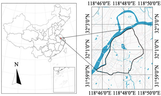
FIGURE 1. Location of the study area.
Three clear Landsat 8 images with little cloud are downloaded from the USGS Data Center (https://earthexplorer.usgs.gov/) for study, and the acquisition dates are May 18th, July 21st, and October 9th in 2017, respectively. Weather conditions of the selected dates and detailed information on the data sets are listed in Table 2. ENVI 5.3 software is applied to perform the data preprocessing including geometric correction, radiometric calibration, atmospheric correction, and clipping of the study area.

TABLE 2. Weather condition of the selected days and detailed information of the Landsat 8 images.
The underlying surface of the study area is divided into four types based on the Landsat data and Baidu Map, namely, UGS, water bodies, buildings, and other rigid pavements. As the research area is in the urban center with little bare land or farmland, except for UGS, water bodies, and buildings, other rigid pavements mainly include open squares and roads.
First, the modified normalized difference water index (MNDWI) is used to extract water from the image, which is proved to be more accurate than the original normalized differential water index (Xu, 2006). The thresholds of each underlying surface are determined based on the original Landsat 8 images and Baidu map after repeated tests of different thresholds and manual calibration. In this study, the threshold of MNDWI is determined as 0.20. Second, the normalized differential vegetation index (NDVI) is used to extract UGSs from the image (Weng et al., 2004). Removing water bodies obtained from the previous steps, the threshold value of 0.35 is used for UGS identification. Third, all the water bodies and UGS are removed, which leaves only the impervious surface. Based on the building footprint information acquired from the Baidu map using Python (Sun et al., 2020), buildings are extracted from the impervious surface. Finally, the remaining pixels are classified as other rigid pavements. As a result, the four types of underlying surface map of the study area are complete. The equations of MNDWI and NDVI are as follows:
where GREEN, MIR, NIR, and RED correspond to the value of bands 3, 6, 5, and 4 of Landsat 8 images, respectively.
This study applied the radiative transfer equation (RTE) to calculate the LST, which is based on the thermal infrared radiative transfer equation by removing the influence of atmosphere on thermal radiation in the process of radiative transfer to accurately obtain the surface temperature (Yu et al., 2014). The RTE has wide applicability and can be applied to the thermal infrared remote sensing data on any sensor; especially, it can achieve the highest LST accuracy in environments with high atmospheric water vapor (Sekertekin, 2019). The calculation is based on Eq. 3:
where
where
The commonly used classification method of LST is the mean–standard deviation method (Sun et al., 2020), which divides different temperature classes according to the mean value and standard deviation of LST in the research area. However, this method may classify more areas as moderate and a much smaller proportion as hot. Taking the LST in July as an example and using the mean–standard deviation method to classify the temperature, the proportion of moderate temperature was 42.29%, and that of high temperature was only 0.49%. In addition, the proportion of each temperature class may vary a lot when comparing different months. Therefore, in order to minimize the error of comparison between months, the quantile method is used to sort all pixels in a certain order and then divide them according to a percentage (Sun et al., 2020). As a result, the data amount of each temperature class, namely, the area of each temperature class is the same. In this study, the LST is divided into seven classes, from low to high, namely, extremely low-temperature class, low-temperature class, sub-low-temperature class, medium-temperature class, sub-high-temperature class, high-temperature class, and extremely high-temperature class. For the sake of concise expression, cls_1 to cls_7 is used as the abbreviation of each class, in which the cls_1 is the extremely low-temperature class and cls_7 is the extremely high-temperature class. The steps are to import the raster map of LST into ArcGIS, and use the quantile method in the reclassify tool to classify the raster into seven classes.
Five landscape metrics were selected to calculate the landscape pattern of different temperature classes as different types of patches (shown in Table 3). The coefficient of variation (CV) of the landscape metric is calculated to intuitively compare the differences between each temperature class in different months. The calculation method of CV is the standard deviation divided by average value, which is not affected by scale and dimension, and can be used to reflect the dispersion degree of a group of data (Lee and Stat, 1994). Similarly, different types of intersection areas are taken as patches to calculate the landscape pattern of each intersection area.
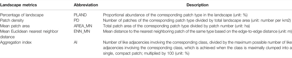
TABLE 3. Selected landscape metrics (Marks, 1995).
The overlap degree in each class of July and May as well as that of July and October is calculated by taking the LST classes of July as the baseline using the intersect tool in ArcGIS, in which the overlapped areas of the same class and different classes are subdivided. The higher the overlap degree of the same class in 2 months, the higher the similarity of the LST distribution in these 2 months. Meanwhile, the proportion of different underlying surfaces in each overlapped area is calculated to analyze the reasons for these differences. Then, the overlapped types of different temperature classes are divided into cold–hot overlapped type and hot–cold overlapped type. The cold–hot overlapped type refers to the area belonging to the lower temperature class in July that overlap with that belonging to the higher temperature class in another month, and the hot–cold overlapped type is the opposite. Moreover, the difference between the two overlapped types in different temperature classes is analyzed.
In order to clarify the thermal impact of each underlying surface in different areas, the land contribution index (LCI) introduced by Huang et al. (2019) is calculated for comparison. The LCI is a quantitative indicator for determining the thermal contribution of the respective underlying surface to the temperature change of the entire area. It considers the temperature difference of each underlying surface and its proportion to the area into consideration shown as follows:
where
The analysis framework of this study is shown in Figure 2. In short, the LST of each month is classified into different classes, and then the LST classes of July are intersected with those of the other 2 months and categorized into different types. Meanwhile, the landscape pattern and underlying surface of each temperature class and intersection area are analyzed.
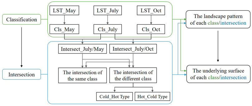
FIGURE 2. Analysis framework.
The LST classes in different months and the temperature range in each class are shown in Figure 3; Table 4. The temperature is highest in July, followed by May and then October. It is clear that the distribution of LST classes in different months has similar patterns in general. The cold island effect is significant near Zijin Mountian, Xuanwu Lake, Mufu Mountain, and other large mountains and water bodies. In May, the heat island effect is more prominent in the northwest area, while it aggregates in the city center area in July. However, in October, the heat islands are relatively small and scattered in the central area but more intense in the southeast and southwest areas.
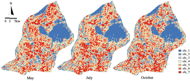
FIGURE 3. LST classes in different months.
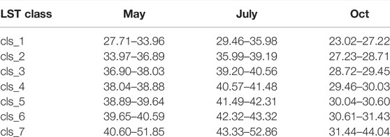
TABLE 4. Temperature range of each temperature class in different months (unit: °C).
The variation coefficients of different LST classes in each month are shown in Table 5. The specific value of each landscape metric is shown in Supplementary Appendix Table A1. The larger the CV is, the higher the dispersion degree of this set of data is, that is, the greater difference in the landscape metric of this LST class in different months. According to the result, the CV of PD, AREA_MN, and ENN_MN are the highest in cls_1, that is, the extremely low-temperature class, while the CV of PLAND and AI are much smaller. It is indicated that the density, area, and distance of patches in the extremely cold area vary greatly from month to month, while the proportion and aggregation degree of patches have no remarkable difference. The CV of cls_6 and cls_7, that is, the high-temperature area and the extremely high-temperature area, is relatively small in all landscape metrics, that is to say, the landscape pattern of the hot area in different months is close to each other. Moreover, cls_3 and cls_4, that is, the sub-low-temperature area and the medium-temperature area, show a higher degree of variances in all metrics, while cls_2 and cls_5, that is, the low-temperature area and the sub-high-temperature area, show a lower degree of difference. In general, the landscape pattern of each temperature class in 3 months present great differences in the area with the lowest temperature and the area with the medium temperature, while there is little difference in the area with high temperature, that is, the area with strong heat island intensity.
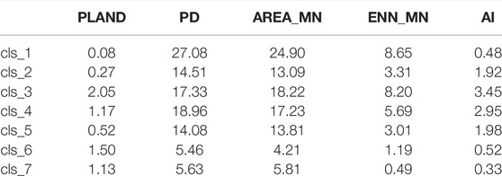
TABLE 5. CV of landscape metrics of different temperature classes in 3 months (unit: %).
Particularly, PLAND has the smallest CV among the 5 landscape metrics, which is reasonable due to the principle of the quantile classification method applied in this study. The CV of PD and AREA_MN is the largest, especially in the cls_1 to cls_5 areas, in which the CV of cls_1 is the largest. Combined with actual data, in October, the PD is always the highest and the AREA_MN is always the lowest among 3 months in all classes. Meanwhile, the difference between July and May is small, in which the PD in July is the lowest and the AREA_MN in July is the highest or slightly lower than in May.
With regard to the ENN_MN, the CV of ENN_MN is the highest in cls_1 and cls_3, while lowest in cls_7. The value of ENN_MN in July is the highest in cls_1 to cls_5, while slightly lower than that in other months in cls_6 and cls_7. The CV of AI is generally small, among which the CV of cls_3 is the highest and cls_7 is the lowest. In cls_2 to cls_5, where the CV is relatively high, AI in October is the smallest, and AI in July is the largest. Only in cls_4, AI in May is slightly higher than that in July.
In conclusion, the difference in landscape patterns between May and July is small but more obvious between July and October, especially the PD and AREA_MN are significantly varied among 3 months. The discrepancy is mostly reflected in the extremely cold area and the area with medium temperature, while not so remarkable in the hot area. Based on the meaning and the concrete value of each landscape metric, it is demonstrated that the LST classes in October are a large number of small patches densely distributed compared with the other 2 months, while LST classes in July and May are quite the opposite.
The type of the underlying surfaces and their proportions in each LST class is calculated as shown in Figure 4. With the rising temperature, the proportion of UGS in each LST class reduces gradually, while the proportion of buildings increases. The proportion of other rigid pavement first increases then slightly reduces. Water bodies are mainly distributed in cls_1 and cls_2, especially in the former. In the extremely low-temperature class, the proportion of UGS is the highest, more than 80%, followed by water, around 11%, and the proportion of buildings is the lowest, which is 2.48% in October and less than 1% in May and July. In the extremely high-temperature class, the proportion of UGS is the lowest, ranging from 5 to 8%; buildings account for more than 60%, and other rigid pavement accounts for about 27%.
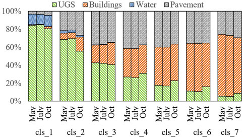
FIGURE 4. Underlying surfaces of different temperature classes in 3 months.
By comparing the proportion of underlying surfaces in the same LST class between different months, it is shown that there is a slight variance between May and July, which is between 0 and 1.31%, while the high difference of up to 13.67% is found between July and October.
As for each underlying surface, the proportion of UGS in cls_1 to cls_3 in October is significantly lower than that in the other 2 months, while in cls_4 to cls_7, it is completely the opposite. In cls_1 to cls_3, the proportion of buildings in October is higher than that in May and July. In cls_4, the proportion of buildings in 3 months is the same, and in cls_5 to cls_7, the proportion of buildings is lower than that in May and July. The water bodies are mainly distributed in cls_1 and cls_2, in which the proportion of water bodies in cls_1 is higher in October than that in the other 2 months, while in cls_2, it is just the reverse. As for the other rigid pavements, the proportion in cls_1, cls_2, and cls_7 is the highest in October, while in cls_3 to cls_6, the proportion in October is the lowest among 3 months.
The LCI of each underlying surface in the entire area and each temperature class is shown in Figure 5. Figure 5A shows the LCI of each underlying surface in the entire area and Figures 5B–D show the LCI of each underlying surface in each temperature class of May, July, and October, respectively. It is clear that UGS and water are the prominent cooling surfaces, while buildings and pavement are the opposite. Because the research area is the central part of the city with mountains and lakes, such as Zijin Mountain and Xuanwu Lake, which play a remarkable role in cooling the area, the LCI of UGS and water are significantly high in this study, especially in July, reaching up to 0.94 for UGS. The LCI of each underlying surface in July is the highest and lowest in October, indicating that the underlying surfaces have a more obvious impact on LST in the summer.
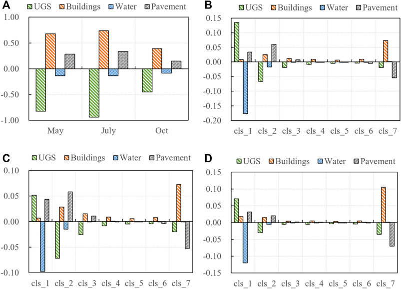
FIGURE 5. LCI of each underlying surface in the whole area (A) and in each LST class in May (B), July (C), and October (D).
However, there are a few differences comparing LCI between each temperature class. In cls_1, only the LCI of water is a negative number and has the highest value; UGS, buildings, and pavement are all positive numbers. In cls_2, the LCI of water lowers a lot, and the LCI of UGS turns to be negative with the highest value. That is to say, the water bodies are prominent in mitigating heat in the extremely low-temperature area, while the cooling effect of UGS is more significant in the low-temperature area. The LCI in cls_3 to cls_6 is much lower than that in the first two classes. In cls_7, buildings have the highest positive value, while the other surfaces have negative value, meaning that buildings are the dominant heating surfaces in the highest temperature area, and even the pavement contributes to a cooling impact compared with buildings in this area. In general, water bodies have a positive effect on cooling down the corresponding area, and buildings have a significant warming effect in all classes, while the cooling effect of UGS is more remarkable in cls_2 to cls_6, especially in cls_2. As for the other rigid pavement, its thermal contribution is warming up the area in cls_1 to cls_3, then turning to cool down the area in cls_4 to cls_7, and the high values are in cls_2 and cls_7. Comparing different months, it is indicated that the LCI of each underlying surface in May is the highest in cls_1, cls_2, and cls_4 to cls_6. In cls_3, the highest LCI is in July, and in cls_7, it is in October. It is shown that the thermal contribution of each underlying surface in different temperature classes is distinguished in different months.
Taking the LST classes of July as the benchmark, the intersection of each class between May and July (intersection_July/May) as well as July and October (intersection_July/Oct) are analyzed, respectively, as shown in Figure 6. The colors in the figure represent different LST classes, in which the color red means high temperature and the color blue means low temperature. The middle column in the figure is the LST class in July, and the upper and lower sides illustrate the LST classes of May and October that overlap with the corresponding class of July and their proportions, respectively. For example, 48.86% of cls_3 in July overlaps with cls_3 in May, which is the overlap of the same class in these 2 months. Apart from that, the overlap of the different classes represents the differences in the spatial distribution of LST between the 2 months. Particularly, 17.75% of cls_3 in July overlaps with cls_2 in May that can be grouped into hot-cold overlapped type, simply expressed as Jcls3_Mcls2, and 24.85% of cls_3 in July overlap with the cls_4 in May, which is a cold–hot overlapped type, abbreviated as Jcls3_Mcls4.
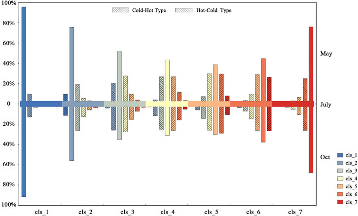
FIGURE 6. Proportions of overlapped areas in different temperature classes in different months.
It is indicated that the overlap degree of the same LST class is higher (58.03%) in the intersection_July/May, while lower (47.12%) in the intersection_July/Oct. As for each LST class, the overlap degree of cls_1, that is, the extremely low-temperature area, is the highest, reaching 92.82% in the intersection_July/May and 88.69% in the intersection_July/Oct. As temperature rises, the overlap degree of the same class first decreases and then increases, presenting a U-shaped trend. The overlap degree of cls_7 is the second highest, 73.18% in the intersection_July/May and 65.01% in the intersection_July/Oct. The overlap degree of cls_5 is the lowest, only 36.00% in the intersection_July/May and 27.54% in the intersection_July/Oct.
The overlapped areas of different LST classes are mainly distributed in one or two adjacent classes before and after this specific class, that is, the cold–hot type and hot–cold type defined in this study. Along with the rising temperature, the proportion of the overlapped area of different temperature classes first increased and then decreased slightly, reaching the highest ratio in cls_5 (27.14%). In the lower temperature class, the cold–hot type is more prevalent, and in the higher temperature class, the hot–cold type is dominant.
In general, the spatial distribution of extremely low-temperature area, low-temperature area, and extremely high-temperature area is similar in different months, while the greatest differences among different months are reflected in the medium temperature area, mainly cls_3 to cls_6, which is the sub-low-temperature area, medium-temperature area, high-temperature area, and sub-high-temperature area.
Taking the intersection area of different classes as the research focus, the landscape metrics of cold–hot and hot–cold overlapped types in the intersection_July/May are compared with those in the intersection_July/Oct, as shown in Table 6. Based on the results, it is indicated that PLAND in the intersection_July/Oct is higher than that in the intersection_July/May, coinciding with the conclusion in the last section. PD of the intersection_July/Oct is much lower than that in the intersection_July/May, while the AREA_MN and AI are the opposite, demonstrating that the difference of the LST class between July and October is presented in larger patches and is more aggregated in the spatial distribution. As for the ENN_MN, the hot–cold type in the intersection_July/Oct is higher than that in the intersection_July/May; however, the cold–hot type is lower than that in the latter, revealing that the distance of the patches in different overlapped types varies a lot in different months.
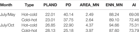
TABLE 6. Landscape metrics of each intersection area.
Furthermore, comparing the difference between the two overlapped types, it is found that the PLAND of the cold–hot type is higher than the hot–cold type in both intersection areas of July/May and July/Oct, indicating that the differences among 3 months can be more categorized into cold–hot type, that is, the colder area in July overlaps with the warmer area in the other 2 months. The PD of the cold–hot type is lower than that in the hot–cold type in the intersection_July/May and higher than that in the latter in the intersection_July/Oct, while the AREA_MN, ENN_MN, and AI are quite the opposite. On the whole, in the intersection_July/May, the patches of cold–hot type are relatively large with a small number and are more aggregated with a longer distance to each other. However, in the intersection_July/Oct, the patches of cold–hot type are relatively small with a large number and are less aggregated with a shorter distance to each other.
The proportions of each underlying surface in the overlapped area of the intersection_July/May are compared with those of the intersection_July/Oct. The results of different overlapped types are shown in Figure 7. It is clear that the differences between the cold–hot overlapped type and the hot–cold overlapped type are obvious. For the hot–cold overlapped type, the proportion of UGS in the intersection_July/May is significantly higher than that in the intersection_July/Oct, while the proportion of buildings is remarkably lower than that in the latter. The proportion of other rigid pavement is lower than that in the latter in cls_2 to cls_4 but higher than that in the latter in the following temperature LST classes. Quite the opposite, in the cold–hot overlapped type, the proportion of UGS in the intersection_July/May is significantly lower than that in intersection_July/Oct, and the proportion of buildings is higher than that in the latter. The proportion of other rigid pavement is higher than that in the latter in cls_1 to cls_3 and lower than that in the latter in the other LST classes.
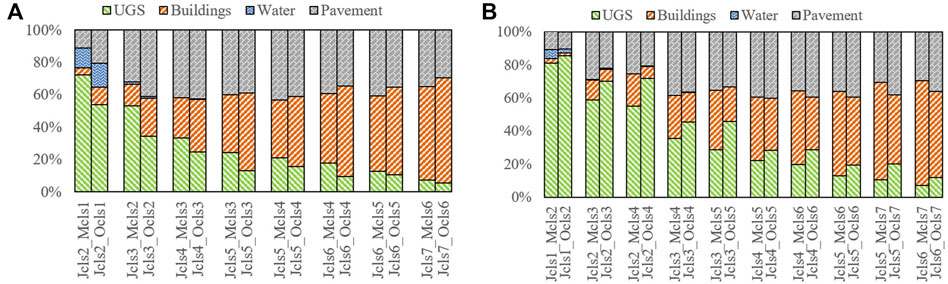
FIGURE 7. Underlying surfaces of (A) hot–cold overlapped type and (B) cold–hot overlapped type in different intersections.
Furthermore, the two overlapped types of different LST classes can be regarded as the differences along with the overall warming or cooling process from May to July to October. From May to July, although the overall temperature has increased, the warming degree of the hot–cold overlapped area is higher than that of other areas, so its LST class in May upgrades when it is in July. Similarly, the cold–hot overlapped type indicates that the warming degree of this area is relatively low, resulting in the downgrading of its LST class. Combined the proportion of each underlying surface in the areas of different overlapped types (Table 7), it is shown that from May to July, buildings account for the most in the cold–hot type and higher than that in the hot–cold type, revealing that buildings have lower warming degree in some extent. The proportion of other rigid pavement is the highest in the hot–cold type and higher than that in the cold–hot type, indicating the warming degree of other rigid pavement is relatively high. In addition, the proportion of water bodies in the hot–cold type is much higher than that in the cold–hot type, demonstrating that water bodies have higher warming degrees from May to July.
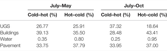
TABLE 7. Proportions of underlying surfaces in different overlapped types.
In the same way, the hot–cold overlapped area can be regarded as the cooling degree of this area is higher than other areas in the process of overall cooling process from July to October, so its LST class downgrades. The cold–hot overlapped type indicates that the cooling degree of this area is lower leading to the upgrading of its LST class. Based on the underlying surface in the intersection_July/Oct, it is shown that the ratio of UGS in the cold–hot overlapped type is significantly higher than that in the hot–cold overlapped area, and the proportions of the building, water bodies as well as other rigid pavements are lower than the latter, suggesting that the last three kinds of underlying surfaces account for more in the area of higher cooling degree, while UGS has a lower cooling degree.
In previous studies, annual and seasonal variation of LST is one of the basic research on urban climate (Peng et al., 2018; Zhang and Wang, 2020; Shi et al., 2021). However, most studies focus on the high or low temperature in the area, namely, the heat islands and cold islands, and little attention is paid to the medium temperature area. According to the aforementioned results, here is a small difference in the high and low temperature areas between different months, while there is a noticeable difference in the medium temperature area. Specifically, the overlap degree of the same LST class in July and May is higher than that in July and October. The highest degree of overlap is in the extremely low-temperature area, followed by the extremely high-temperature area. Along with the increase in temperature, the overlap degree of the same LST class will decrease first and then increase, showing a U-shape change trend, indicating that the distribution of the cold and the hot islands in the city is similar in different months, while that of medium-temperature area significantly differs. One plausible reason is that the LST of medium-temperature area is not only dependent on its ground and spatial feature but also influenced by surrounding heat and cold islands. Although the spatial pattern of heat and cold islands may not significantly change over 3 months, their ability or extent to regulate their surroundings fluctuates over time (Yu et al., 2019; Yu K. et al., 2020).
In this study, the LST differences across time are subdivided into cold–hot and hot–cold overlapped types, and the distinctions between those two types turns out to be significant, in which the cold–hot type accounts for more in both intersections of July/May and July/Oct. Furthermore, in the intersection_July/May, the patches of cold–hot type are relatively large with a small number and more aggregated with a longer distance to each other. However, in the intersection_July/Oct, the landscape pattern of the cold–hot type is quite the opposite. According to the spatial distribution of different overlapped types shown in Figure 8, in the intersection_July/May, most of the cold–hot type areas are distributed densely in the northwest of the research area, and other small parts are scattered in the central area, along the southeast edge and the southwest corner. On the contrary, the hot–cold type areas are mainly located in the east and south of the study area, especially aggregated in the south of Zijin Mountain. In the intersection_July/Oct, the cold–hot type areas are mostly distributed along the surrounding boundary of the study area, while the hot–cold type areas occupy the majority of the city center. In other words, there is a difference in the warming and cooling degrees within the research area, and it needs to be further explored.
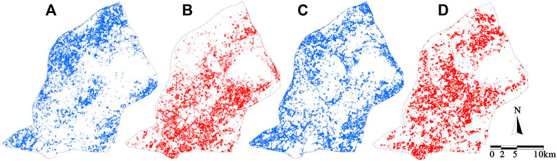
FIGURE 8. Spatial distribution of the (A) cold–hot type in the intersection_July/May, (B) hot–cold type in the intersection_July/May, (C) cold–hot type in the intersection_July/Oct, and (D) hot–cold type in the intersection_July/Oct.
The main reason for the LST difference lies in the variances of underlying surfaces (Liu et al., 2013; Guo et al., 2020; Parvez et al., 2021). It is concluded that UGS and water bodies contribute the most in the cool area, while buildings and other rigid pavements account for the most in the hot area, in which buildings are the dominant factor. However, it is worth noting that UGS occupies around 5% even in the highest temperature area, indicating that UGS may not always be the cold island, and its surrounding environment should be taken into consideration (Yuan et al., 2021). Combined with the LCI of each underlying surface, the results show that the performance of the underlying surface in the whole region is different from that in different temperature classes, indicating that the role of each underlying surface in different temperature areas is different. Both UGS and water bodies contribute a cooling effect to the area, and the LCI of UGS is higher than that of water bodies, but the cooling effect of the latter is more significant in the extremely cool area, while UGS plays a dominant role in the cool area. Previous studies have investigated the cooling effect of UGS and water bodies. Some studies have come to the same conclusion that the LCI of UGS is higher than that of water bodies (Tarawally et al., 2018), while others have obtained the opposite results due to the different research scale (Huang et al., 2019), but few research has further investigated the thermal contribution of underlying surface in different temperature classes. According to Wang et al. (2019), the impact of urban water bodies on the LST does vary across different LCZ types, which supports the aforementioned conclusion to a certain extent. Therefore, specific mitigation and adaption efforts should be made according to the actual conditions.
By comparing the underlying surfaces between different months, it is found that there is little difference between the underlying surface in May and July, but a significant difference between the underlying surface in July and October. In summary, water bodies contribute more to the cooling effect in October, while the contribution degree of UGS in October is relatively lower than that in the other 2 months. In addition, other rigid pavements contribute more to high temperature in October. Furthermore, there are great differences between the two overlapped types. In the hot–cold overlapped type, the proportion of UGS in the intersection_July/May is significantly higher than that in the intersection_July/Oct, while that of the building is significantly lower than that of the latter. The proportion of other rigid pavements is lower than that of the latter in cls_2 to cls_4 but higher than that of the latter in the following LST class. However, in the cold–hot overlapped type, it is totally the opposite case.
Combining with the meaning of the cold–hot and hot–cold overlapped types, that is, the warming and cooling degrees of different underlying surfaces, it is concluded that the warming degree of buildings is relatively low, while other rigid pavements and water bodies have a higher warming degree in certain areas in the warming process from May to July. In the cooling process from July to October, the cooling degree of UGS in some areas is low, while that of buildings, water bodies, and other rigid pavement is higher, especially buildings. Zhang et al. (2021) defined the urban surface heating rate (SHR) as the change in LST per percentage of impervious surface area (ISA) and the urban surface cooling rate (SCR) as the change in LST per percentage of fractional vegetation cover (FVC). They also concluded that the trend of SHR and SCR, along with the percent of ISA and FVC, had remarkable seasonal differences. The difference is that Zhang et al. (2021) considered the specific heating and cooling rate of the underlying surface and its variation trend with temperature within a day, while this study focuses on the heating and cooling degrees of each underlying surface and its variation trend across time. Moreover, the former research did not distinguish the impervious surface between buildings and other rigid pavements, which is proved to have great differences in the influence of the UHI formation in this study.
This study may provide a new perspective on mitigating the UHI effect at the different stages of LST change. In addition to focusing on the UHIs effect at a particular time, temperature changes before and after that particular time, may help understand the formation of the heat island effect. From July to October, the landscape pattern of low- and medium-temperature areas exhibits a trend of fragmentation and decentralization, while the high-temperature area does not significantly change. Conversely, if heat island patches could be more fragmented and decentralized, their intensity might be reduced. Yu et al. (2021) came to a similar conclusion in the research of heat networks, that is, when links and pinch points are blocked, SUHI connectivity is reduced, thus breaking the network and significantly alleviating the SUHI effect. Therefore, effective cooling measures should be taken in high-risk and key areas to prevent corridor connectivity. In other words, heat patches are prevented from being aggregated and linked by fragmenting them into small patches and breaking the linkages. Similarly, Wang et al. (2017) pointed out that large temperature contrasts between adjacent patches and fragmental patches are recommended for heat release.
Considering the significant relationship between LST and underlying surfaces, it is essential to optimize the spatial distribution of underlying surfaces. This study reveals that UGS and water bodies show distinguished thermal contributions to the different temperature classes, which means that the more specific mitigation and adaption efforts should be carried out under different circumstances. It seems that water bodies contribute the highest cooling effect to the coolest area, while UGS has a sustained cooling effect from a cool to a hot area. With limited resources, there might be relative thresholds for both UGS and water bodies to fulfill a win–win cooling efficiency in the whole area (Yu Z. et al., 2020; Wu et al., 2020). Previous studies have generally regarded buildings and other rigid pavements together as impervious surfaces and examined their positive impact on temperature rise (Liu et al., 2016). However, it turns out that buildings contribute the most to the highest temperature area, while other rigid pavement has a relative cooling effect in the same area, even though its thermal contribution in the whole area is the opposite. Therefore, it may be a feasible method to explore more about the properties of other rigid pavements and enhance their cooling effect in high-temperature areas.
There are a few limitations that need to be mentioned. First, this study selects May, July, and October as the representative of different seasons that could be haphazard due to unpredictable weather events. Second, the underlying surfaces are classified based on the Landsat image with 30 m resolution in order to coincide with the LST data, but it is not enough for more detailed research on the characteristics of each underlying surface. Third, this study focuses on the impact of different underlying surface types on LST variation, while other factors such as the vegetation volume in different seasons, energy consumption, and other indexes related to production activities are not involved.
Future studies will detail the characteristics of different underlying surfaces, for example, building height and density, greenspace morphology, the area and shape of water bodies, the impervious rate of other rigid pavement, and the influence of the surrounding environment. Furthermore, the spatial differences between cold–hot and hot–cold overlapped types and their distribution regularities will be thoroughly analyzed based on the detailed aforementioned factors. It is believed that it can provide applicable references for future urban design.
Taking the LST of Nanjing in different months as an example, this study divided temperature into different classes by using the quantile method and then compared the spatial distribution of each LST class in different months. The results indicate that there is a small difference in the distribution of heat and cold islands between months, while a major difference in medium-temperature area. In particular, the spatial pattern of each LST class illustrates a trend of fragmentation and decentralization from July to October. Further analysis of the intersection of each LST class in different months shows that the overlap degree of the low-temperature area and high-temperature area is higher than that of the medium-temperature area. The overlapped area of different LST classes is divided into hot–cold and cold–hot types. In the process of temperature change from May to July and October, different overlapped types can be regarded as different cooling degrees in different areas to a certain extent. It turns out that the warming degree of other rigid pavements is higher in the warming process from May to July, and the cooling degree of buildings is greater in the cooling process from July to October. Meanwhile, the thermal contribution of each underlying surface is different among LST classes, so it is necessary to formulate more targeted strategies. This study provides a new perspective for the mitigation of UHI based on the comprehensive understanding of the temperature change from a continuous-time sequence, expecting to be a reference for sustainable urban design in the future.
The original contributions presented in the study are included in the article/Supplementary Material, further inquiries can be directed to the corresponding author.
XW collected the data, performed data analysis, and developed the draft manuscript as well as the tables and figures. X-JW guided the conceptualization of the study and provided instructions on the research method and revision of the manuscript.
This research was funded by the National Natural Science Foundation of China (50978054 and 51878144).
The authors declare that the research was conducted in the absence of any commercial or financial relationships that could be construed as a potential conflict of interest.
All claims expressed in this article are solely those of the authors and do not necessarily represent those of their affiliated organizations, or those of the publisher, the editors, and the reviewers. Any product that may be evaluated in this article, or claim that may be made by its manufacturer, is not guaranteed or endorsed by the publisher.
The Supplementary Material for this article can be found online at: https://www.frontiersin.org/articles/10.3389/fenvs.2022.872282/full#supplementary-material
Abbas, A., He, Q., Jin, L., Li, J., Salam, A., Lu, B., et al. (2021). Spatio-Temporal Changes of Land Surface Temperature and the Influencing Factors in the Tarim Basin, Northwest China. Remote Sensing. 13 (19), 3792. doi:10.3390/rs13193792
Anderson, G. B., and Bell, M. L. (2011). Heat Waves in the United States: Mortality Risk during Heat Waves and Effect Modification by Heat Wave Characteristics in 43 U.S. Communities. Environ. Health Perspect. 119 (2), 210–218. doi:10.1289/ehp.1002313
Chao, Z., Wang, L., Che, M., and Hou, S. (2020). Effects of Different Urbanization Levels on Land Surface Temperature Change: Taking Tokyo and Shanghai for Example. Remote Sensing. 12 (12), 2022. doi:10.3390/rs12122022
Chen, A., Yao, X. A., Sun, R., and Chen, L. (2014). Effect of Urban green Patterns on Surface Urban Cool Islands and Its Seasonal Variations. Urban For. Urban Green. 13 (4), 646–654. doi:10.1016/j.ufug.2014.07.006
Chen, Q., Cheng, Q., Chen, Y., Li, K., Wang, D., and Cao, S. (2021). The Influence of Sky View Factor on Daytime and Nighttime Urban Land Surface Temperature in Different Spatial-Temporal Scales: A Case Study of Beijing. Remote Sensing. 13 (20), 4117. doi:10.3390/rs13204117
Das, M., and Das, A. (2020). Assessing the Relationship Between Local Climatic Zones (Lczs) and Land Surface Temperature (Lst) – a Case Study of Sriniketan-Santiniketan Planning Area (Sspa), West Bengal, India. Urban Clim. 32, 100591. doi:10.1016/j.uclim.2020.100591
Desa, U. (2019). World Population Prospects 2019: Highlights. New York, NY: United Nations Department for Economic and Social Affairs.
Du, H., Cai, W., Xu, Y., Wang, Z., Wang, Y., and Cai, Y. (2017). Quantifying the Cool Island Effects of Urban green Spaces Using Remote Sensing Data. Urban For. Urban Green. 27, 24–31. doi:10.1016/j.ufug.2017.06.008
Dudorova, N. V., and Belan, B. D. (2019). “The Role of Evaporation and Condensation of Water in the Formation of the Urban Heat Island,” in 25th International Symposium On Atmospheric and Ocean Optics - Atmospheric Physics).
Ebi, K. L., Capon, A., Berry, P., Broderick, C., de Dear, R., Havenith, G., et al. (2021). Hot Weather and Heat Extremes: Health Risks. The Lancet. 398 (10301), 698–708. doi:10.1016/s0140-6736(21)01208-3
Elmes, A., Rogan, J., Williams, C., Ratick, S., Nowak, D., and Martin, D. (2017). Effects of Urban Tree Canopy Loss on Land Surface Temperature Magnitude and Timing. Isprs J. Photogrammetry Remote Sensing. 128, 338–353. doi:10.1016/j.isprsjprs.2017.04.011
Erdem, U., Cubukcu, K. M., and Sharifi, A. (2021). An Analysis of Urban Form Factors Driving Urban Heat Island: the Case of Izmir. Environ. Dev. Sustain. 23 (5), 7835–7859. doi:10.1007/s10668-020-00950-4
Ghosh, S., and Das, A. (2018). Modelling Urban Cooling Island Impact of green Space and Water Bodies on Surface Urban Heat Island in a Continuously Developing Urban Area. Model. Earth Syst. Environ. 4 (2), 501–515. doi:10.1007/s40808-018-0456-7
Guha, S., Govil, H., Gill, N., and Dey, A. (2021). A Long-Term Seasonal Analysis on the Relationship between LST and NDBI Using Landsat Data. Quat. Int. 575-576, 249–258. doi:10.1016/j.quaint.2020.06.041
Guha, S., and Govil, H. (2020). Seasonal Impact on the Relationship between Land Surface Temperature and Normalized Difference Vegetation index in an Urban Landscape. Geocarto Int., 1–21. doi:10.1080/10106049.2020.1815867
Guo, A., Yang, J., Sun, W., Xiao, X., Xia Cecilia, J., Jin, C., et al. (2020). Impact of Urban Morphology and Landscape Characteristics on Spatiotemporal Heterogeneity of Land Surface Temperature. Sustainable Cities Soc. 63, 102443. doi:10.1016/j.scs.2020.102443
He, B.-J., Ding, L., and Prasad, D. (2020). Relationships Among Local-Scale Urban Morphology, Urban Ventilation, Urban Heat Island and Outdoor thermal comfort under Sea Breeze Influence. Sustainable Cities Soc. 60, 102289. doi:10.1016/j.scs.2020.102289
He, B.-J., Wang, J., Zhu, J., and Qi, J. (2022). Beating the Urban Heat: Situation, Background, Impacts and the Way Forward in China. Renew. Sustainable Energ. Rev. 161, 112350. doi:10.1016/j.rser.2022.112350
Huang, M., Cui, P., and He, X. (2018). Study of the Cooling Effects of Urban Green Space in Harbin in Terms of Reducing the Heat Island Effect. Sustainability. 10 (4), 1101. doi:10.3390/su10041101
Huang, Q., Huang, J., Yang, X., Fang, C., and Liang, Y. (2019). Quantifying the Seasonal Contribution of Coupling Urban Land Use Types on Urban Heat Island Using Land Contribution Index: A Case Study in Wuhan, China. Sustainable Cities Soc. 44, 666–675. doi:10.1016/j.scs.2018.10.016
Jay, O., Capon, A., Berry, P., Broderick, C., de Dear, R., Havenith, G., et al. (2021). Reducing the Health Effects of Hot Weather and Heat Extremes: from Personal Cooling Strategies to green Cities. The Lancet. 398 (10301), 709–724. doi:10.1016/s0140-6736(21)01209-5
Kong, F., Yin, H., James, P., Hutyra, L. R., and He, H. S. (2014). Effects of Spatial Pattern of Greenspace on Urban Cooling in a Large Metropolitan Area of Eastern China. Landscape Urban Plann. 128, 35–47. doi:10.1016/j.landurbplan.2014.04.018
Lee, E. W. T., and Stat, A. (1994). “Transformation of the Coefficient of Variation,” in Spring Meeting of the Eastern-North-American-Region of the Biometric-Society), 355–358.
Li, X., and Zhou, W. (2019). Optimizing Urban Greenspace Spatial Pattern to Mitigate Urban Heat Island Effects: Extending Understanding from Local to the City Scale. Urban For. Urban Green. 41, 255–263. doi:10.1016/j.ufug.2019.04.008
Liu, K., Gao, W., Gu, X. F., and Gao, Z. Q. (2013). “The Relation between the Urban Heat Island Effect and the Underlying Surface LUCC of Meteorological Stations,” in Conference on Remote Sensing and Modeling of Ecosystems for Sustainability X).
Liu, K., Su, H., Li, X., Wang, W., Yang, L., and Liang, H. (2016). Quantifying Spatial-Temporal Pattern of Urban Heat Island in Beijing: An Improved Assessment Using Land Surface Temperature (LST) Time Series Observations from LANDSAT, MODIS, and Chinese New Satellite GaoFen-1. IEEE J. Sel. Top. Appl. Earth Observations Remote Sensing. 9 (5), 2028–2042. doi:10.1109/jstars.2015.2513598
Makhelouf, A. (2009). The Effect of Green Spaces on Urban Climate and Pollution. Iranian J. Environ. Health Sci. Eng. 6 (1), 35–40. Available at: https://ijehse.tums.ac.ir/index.php/jehse/article/view/190.
Markevych, I., Schoierer, J., Hartig, T., Chudnovsky, A., Hystad, P., Dzhambov, A. M., et al. (2017). Exploring Pathways Linking Greenspace to Health: Theoretical and Methodological Guidance. Environ. Res. 158, 301–317. doi:10.1016/j.envres.2017.06.028
Marks, K. M. B. J. (1995). FRAGSTATS: Spatial Pattern Analysis Program for Quantifying Landscape Structure. Portland, OR: USDA Forest Service.
Masoudi, M., and Tan, P. Y. (2019). Multi-year Comparison of the Effects of Spatial Pattern of Urban green Spaces on Urban Land Surface Temperature. Landscape Urban Plann. 184, 44–58. doi:10.1016/j.landurbplan.2018.10.023
Mazdiyasni, O., and AghaKouchak, A. (2015). Substantial Increase in Concurrent Droughts and Heatwaves in the United States. Proc. Natl. Acad. Sci. U.S.A. 112 (37), 11484–11489. doi:10.1073/pnas.1422945112
Nanjing Bureau of Statistics (2019). Statistical Yearbook of Nanjing. Nanjing, China: China Statistics Press.
Oke, T. R. (1982). The Energetic Basis of the Urban Heat Island. Q.J R. Met. Soc. 108 (455), 1–24. doi:10.1002/qj.49710845502
Parvez, I. M., Aina, Y. A., and Balogun, A.-L. (2021). The Influence of Urban Form on the Spatiotemporal Variations in Land Surface Temperature in an Arid Coastal City. Geocarto Int. 36 (6), 640–659. doi:10.1080/10106049.2019.1622598
Peng, J., Jia, J., Liu, Y., Li, H., and Wu, J. (2018). Seasonal Contrast of the Dominant Factors for Spatial Distribution of Land Surface Temperature in Urban Areas. Remote Sensing Environ. 215, 255–267. doi:10.1016/j.rse.2018.06.010
Rasul, A., Balzter, H., and Smith, C. (2015). Spatial Variation of the Daytime Surface Urban Cool Island during the Dry Season in Erbil, Iraqi Kurdistan, from Landsat 8. Urban Clim. 14, 176–186. doi:10.1016/j.uclim.2015.09.001
Sekertekin, A. (2019). Validation of Physical Radiative Transfer Equation-Based Land Surface Temperature Using Landsat 8 Satellite Imagery and SURFRAD In-Situ Measurements. J. Atmos. Solar-Terrestrial Phys. 196, 105161. doi:10.1016/j.jastp.2019.105161
Shi, L., Ling, F., Foody, G. M., Yang, Z., Liu, X., and Du, Y. (2021). Seasonal SUHI Analysis Using Local Climate Zone Classification: A Case Study of Wuhan, China. Int. J. Environ Res Public Health. 18 (14), 7242. doi:10.3390/ijerph18147242
Stanganelli, M., and Gerundo, C. (2017). Understanding the Role of Urban Morphology and Green Areas Configuration during Heat Waves. Int. J. Agric. Environ. Inf. Syst. 8 (2), 50–64. doi:10.4018/ijaeis.2017040104
Stewart, I. D., and Oke, T. R. (2012). Local Climate Zones for Urban Temperature Studies. Bull. Am. Meteorol. Soc. 93 (12), 1879–1900. doi:10.1175/bams-d-11-00019.1
Sun, L., Tang, L., Shao, G., Qiu, Q., Lan, T., and Shao, J. (2020). A Machine Learning-Based Classification System for Urban Built-Up Areas Using Multiple Classifiers and Data Sources. Remote Sensing. 12 (1), 91. doi:10.3390/rs12010091
Sun, Y., Gao, C., Li, J., Wang, R., and Liu, J. (2019). Quantifying the Effects of Urban Form on Land Surface Temperature in Subtropical High-Density Urban Areas Using Machine Learning. Remote Sensing. 11 (8), 959. doi:10.3390/rs11080959
Tarawally, M., Xu, W., Hou, W., and Mushore, T. (2018). Comparative Analysis of Responses of Land Surface Temperature to Long-Term Land Use/Cover Changes between a Coastal and Inland City: A Case of Freetown and Bo Town in Sierra Leone. Remote Sensing. 10 (1), 112. doi:10.3390/rs10010112
United Nation (2021). The Impact of Disasters and Crises on Agriculture and Food Security. Food Agric. Org. Unit Nations. 8, 94–95. Available at: http://www.fao.org/3/cb3673en/cb3673en.pdf.
Van Ryswyk, K., Prince, N., Ahmed, M., Brisson, E., Miller, J. D., and Villeneuve, P. J. (2019). Does Urban Vegetation Reduce Temperature and Air Pollution Concentrations? Findings from an Environmental Monitoring Study of the Central Experimental Farm in Ottawa, Canada. Atmos. Environ. 218, 116886. doi:10.1016/j.atmosenv.2019.116886
Vulova, S., and Kleinschmit, B. (2019). “Therma Lbehavior and its Seasonal and Diurnal Variability of Urban green Infrastructure in a Mid-latitude City - Berlin,” in 2019 Joint Urban Remote Sensing Event (JURSE). doi:10.1109/jurse.2019.8809011
Wang, X., Wei, X., and Zou, H. (2020. Research Progress About the Impact of Urban Green Space Spatial Pattern on Urban Heat Island Ecol. Environ. Sci. 29 (9), 1904–1911. doi:10.16258/j.cnki.1674-5906.2020.09.024
Wang, Y., Zhan, Q., and Ouyang, W. (2019). How to Quantify the Relationship between Spatial Distribution of Urban Waterbodies and Land Surface Temperature? Sci. Total Environ. 671, 1–9. doi:10.1016/j.scitotenv.2019.03.377
Wang, Y., Zhan, Q., and Ouyang, W. (2017). Impact of Urban Climate Landscape Patterns on Land Surface Temperature in Wuhan, China. Sustainability. 9 (10), 1700. doi:10.3390/su9101700
Weng, Q., Lu, D., and Schubring, J. (2004). Estimation of Land Surface Temperature-Vegetation Abundance Relationship for Urban Heat Island Studies. Remote Sensing Environ. 89 (4), 467–483. doi:10.1016/j.rse.2003.11.005
Wu, J., Yang, S., and Zhang, X. (2020). Interaction Analysis of Urban Blue-Green Space and Built-Up Area Based on Coupling Model-A Case Study of Wuhan Central City. Water. 12 (8), 2185. doi:10.3390/w12082185
Xu, G., Chen, L., Chen, Y., Wang, T., Shen, F.-H., Wang, K., et al. (2020). Impact of Heatwaves and Cold Spells on the Morbidity of Respiratory Diseases: A Case Study in Lanzhou, China. Phys. Chem. Earth, Parts A/B/CParts A/B/C. 115, 102825. doi:10.1016/j.pce.2019.102825
Xu, H. (2006). Modification of Normalised Difference Water index (NDWI) to Enhance Open Water Features in Remotely Sensed Imagery. Int. J. Remote Sensing. 27 (14), 3025–3033. doi:10.1080/01431160600589179
Xu, X., Liu, S., Sun, S., Zhang, W., Liu, Y., Lao, Z., et al. (2019). Evaluation of Energy Saving Potential of an Urban green Space and its Water Bodies. Energy and Buildings. 188-189, 58–70. doi:10.1016/j.enbuild.2019.02.003
Yu, K., Chen, Y., Liang, L., Gong, A., and Li, J. (2020). Quantitative Analysis of the Interannual Variation in the Seasonal Water Cooling Island (WCI) Effect for Urban Areas. Sci. Total Environ. 727, 138750. doi:10.1016/j.scitotenv.2020.138750
Yu, Z., Yang, G., Zuo, S., Jørgensen, G., Koga, M., and Vejre, H. (2020). Critical Review on the Cooling Effect of Urban Blue-green Space: A Threshold-Size Perspective. Urban For. Urban Green. 49, 126630. doi:10.1016/j.ufug.2020.126630
Yu, K., Chen, Y., Wang, D., Chen, Z., Gong, A., and Li, J. (2019). Study of the Seasonal Effect of Building Shadows on Urban Land Surface Temperatures Based on Remote Sensing Data. Remote Sensing. 11 (5), 497. doi:10.3390/rs11050497
Yu, X., Guo, X., and Wu, Z. (2014). Land Surface Temperature Retrieval from Landsat 8 TIRS-Comparison between Radiative Transfer Equation-Based Method, Split Window Algorithm, and Single Channel Method. Remote Sensing. 6 (10), 9829–9852. doi:10.3390/rs6109829
Yu, Z., Guo, X., Zeng, Y., Koga, M., and Vejre, H. (2018). Variations in Land Surface Temperature and Cooling Efficiency of green Space in Rapid Urbanization: The Case of Fuzhou City, China. Urban For. Urban Green. 29, 113–121. doi:10.1016/j.ufug.2017.11.008
Yu, Z., Zhang, J., and Yang, G. (2021). How to Build a Heat Network to Alleviate Surface Heat Island Effect? Sustainable Cities Soc. 74, 103135. doi:10.1016/j.scs.2021.103135
Yuan, B., Zhou, L., Dang, X., Sun, D., Hu, F., and Mu, H. (2021). Separate and Combined Effects of 3D Building Features and Urban green Space on Land Surface Temperature. J. Environ. Manage. 295, 113116. doi:10.1016/j.jenvman.2021.113116
Zhang, S. N., and Wang, P. (2021). “Impact of Urban Form on Land Surface Temperature (LST) Based Seasonal Characteristics: Empirical Study from Nanjing,” in 6th International Conference on Advances in Energy Resources and Environment Engineering (ICAESEE)).
Zhang, X., Wang, D., Hao, H., Zhang, F., and Hu, Y. (2017). Effects of Land Use/Cover Changes and Urban Forest Configuration on Urban Heat Islands in a Loess Hilly Region: Case Study Based on Yan'an City, China. Int. J. Environ Res Public Health. 14 (8), 840. doi:10.3390/ijerph14080840
Zhang, Y., Zhan, Y., Yu, T., and Ren, X. (2017). Urban green Effects on Land Surface Temperature Caused by Surface Characteristics: A Case Study of Summer Beijing Metropolitan Region. Infrared Phys. Technology 86, 35–43. doi:10.1016/j.infrared.2017.08.008
Zhang, Y., Balzter, H., and Li, Y. (2021). Influence of Impervious Surface Area and Fractional Vegetation Cover on Seasonal Urban Surface Heating/Cooling Rates. Remote Sensing. 13 (7), 1263. doi:10.3390/rs13071263
Zhao, C., Fu, G., Liu, X., and Fu, F. (2011). Urban Planning Indicators, Morphology and Climate Indicators: A Case Study for a north-south Transect of Beijing, China. Building Environ. 46 (5), 1174–1183. doi:10.1016/j.buildenv.2010.12.009
Zhao, Z., Sharifi, A., Dong, X., Shen, L., and He, B.-J. (2021). Spatial Variability and Temporal Heterogeneity of Surface Urban Heat Island Patterns and the Suitability of Local Climate Zones for Land Surface Temperature Characterization. Remote Sensing. 13 (21), 4338. doi:10.3390/rs13214338
Zhou, D., Zhang, L., Li, D., Huang, D., and Zhu, C. (2016). Climate-vegetation Control on the Diurnal and Seasonal Variations of Surface Urban Heat Islands in China. Environ. Res. Lett. 11 (7), 074009. doi:10.1088/1748-9326/11/7/074009
Zhou, W., Qian, Y., Li, X., Li, W., and Han, L. (2014). Relationships between Land Cover and the Surface Urban Heat Island: Seasonal Variability and Effects of Spatial and Thematic Resolution of Land Cover Data on Predicting Land Surface Temperatures. Landscape Ecol. 29 (1), 153–167. doi:10.1007/s10980-013-9950-5
Keywords: land surface temperature, spatial distribution, urban heat island, underlying surfaces, classification, intersection, land contribution index
Citation: Wei X and Wang X-J (2022) Analyzing the Spatial Distribution of LST and Its Relationship With Underlying Surfaces in Different Months by Classification and Intersection. Front. Environ. Sci. 10:872282. doi: 10.3389/fenvs.2022.872282
Received: 09 February 2022; Accepted: 30 March 2022;
Published: 02 May 2022.
Edited by:
Zhaowu Yu, Fudan University, ChinaCopyright © 2022 Wei and Wang. This is an open-access article distributed under the terms of the Creative Commons Attribution License (CC BY). The use, distribution or reproduction in other forums is permitted, provided the original author(s) and the copyright owner(s) are credited and that the original publication in this journal is cited, in accordance with accepted academic practice. No use, distribution or reproduction is permitted which does not comply with these terms.
*Correspondence: Xiao-Jun Wang, eGp3b3JraW5nQDE2My5jb20=
Disclaimer: All claims expressed in this article are solely those of the authors and do not necessarily represent those of their affiliated organizations, or those of the publisher, the editors and the reviewers. Any product that may be evaluated in this article or claim that may be made by its manufacturer is not guaranteed or endorsed by the publisher.
Research integrity at Frontiers
Learn more about the work of our research integrity team to safeguard the quality of each article we publish.