 Yufei Ding
 Xingnian Liu
94% of researchers rate our articles as excellent or good
Learn more about the work of our research integrity team to safeguard the quality of each article we publish.
Find out more
ORIGINAL RESEARCH article
Front. Environ. Sci., 01 March 2022
Sec. Freshwater Science
Volume 10 - 2022 | https://doi.org/10.3389/fenvs.2022.858692
This article is part of the Research TopicThe Urban Fluvial and Hydro-Environment SystemView all 21 articles
Compared with floods occurring over plains, alpine flash floods are formed over scattered locations with complex terrain and data is often lacking regarding the land topography, flow and sedimentation, causing difficulties when developing mathematical models to predict flash floods. The existing flash flood models mainly focus on the influence of water flow, such as the sharp increase in flow discharge caused by convergence at steep slopes, disregarding the sediment load carried by the water flow. However, under the effect of high-intensity sediment transport, the sedimentation in gullies may lead to surges in water level, causing the phenomenon of “great disasters resulting from minor flooding”. In this study, an efficient and accurate water-sediment coupling model was established with a Godunov-type finite volume method based 2D flow model, and a sediment module and OPENMP parallel computing module were added as well. Firstly, a common gully in mountainous area with large gradient variations was used as a generalized model to explore the impact of sedimentation on the flow field of the gully and compared with the physical model. Then, the alpine flash flood incident in Gengdi Village was simulated with the computer model. The calculation results show that the high-intensity sedimentation significantly increased the magnitude of alpine flash floods. Calculated by this mathematical model, the research results verified that this mathematic model can efficiently, accurately and concisely predict the occurrence of flash floods in gullies with large gradient variations. The model also provides a flow and sediment modeling method that incorporates the effect of high-intensity sediment transport into the traditional flash flood flow model. Thus, this model can be a powerful tool for detecting flash floods.
Short-term high-intensity rainfall may cause flash flooding in mountainous regions, bringing large amounts of sediment (Reid et al., 1998). The situation can rapidly evolve into natural disasters such as landslides and mudslides, causing huge destructions such as the collapse of bridges, damage to buildings, traffic interruptions, and casualties (Hapuarachchi et al., 2011). Flood waters mixed with large amounts of sediment flows into the gully, absorbing energy from the flow which leads to increased flow resistance. Meanwhile, the sediment load in the flash flood is greater than the sediment-carrying capacity of the water flow. As a result, sediment deposits and quickly builds up in certain areas, resulting in an increase in water level, which endangers the buildings on the river bank, leading to the phenomenon that minor floods can cause great disasters. Every year in China, the loss of life and property caused by flash floods accounts for about 40% of the total loss caused by natural disasters. As shown in Figure 1, the annual average death toll from flash floods during 2009–2018 was 608, accounting for 78.1% of the death toll from floods. In 2010, the catastrophic debris flow disaster in Zhouqu, Gansu caused 1,744 deaths and a direct economic loss of 0.4 billion CNY (Ministry of water resources of the people’s republic of China, 2018). As flash floods often occur suddenly in remote mountainous regions that are lacking in observational data, there is a great degree of technical difficulty and uncertainty in evaluating pre-disaster risk, or for monitoring, providing early alerts and planning for post-disaster emergency rescue. The key to lessening the destruction caused by flash floods is to provide accurate and early alerts in time to take remedial actions and respond to the disaster.
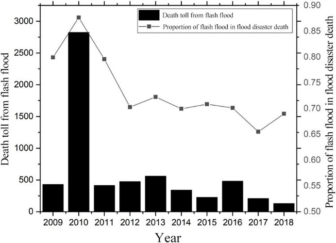
FIGURE 1. The number of people affected by flash floods during 2009–1018.
America, Britain, Australia and China have taken the lead in studying the mechanism of flash floods and forecasting their occurrence (Penning-Rowsell et al., 2000; Handmer, 2001; Liu et al., 2018; Shan et al., 2018). As more knowledge was gained regarding the mechanism, it became clear that establishing an efficient and reliable flash flood numerical model is of great significance for the accurate forecasting of flash floods. The current trend is to establish a 1D or 2D hydraulic model for areas vulnerable to flash flooding. The hydraulic model is mainly based on shallow water equations and uses the Saint-Venant equations for fluid calculations (Piotrowski et al., 2006). Norbiato et al. (2007) used the CARIMA 1D unsteady flow model to reproduce the catastrophic flash floods that occurred in the Gard region of France in September 2002, and they calculated the peak flow at each key station during the flash flooding. Kobold and Brilly (2006) used a 1D numerical model to evaluate the impact of open-channel flash floods on riverbeds and dams in mountainous areas. Om (1976) used clear water scouring and high-intensity sediment input to carry out 1D numerical simulations on alpine rivers with steep slopes, and they analyzed the post-flood longitudinal deposition form. Compared with 2D models, 1D models require less data, calculation time and computer memory. However, 1D models cannot accurately calculate the hydraulic elements when there are large and irregular changes in the terrain of the alpine rivers. As a result, the results from flash floods simulations have been poor (Sirdaş and Şen, 2007).
2D models can provide some calculations for river channel flow fields under flash flooding, such as the flow depth and velocity vector at each grid point, and the flow field can also be accurately simulated with high accuracy without the need to interpolate by refining the grid. The finite element method and the finite volume method are numerical modeling methods commonly used for 2D water flow simulations. In the finite element method, there is freedom to choose the basic functions that will be used, and elements of various shapes can be used to fit the complex geometric shapes. In addition, simulation accuracy can be improved by establishing higher-order polynomials in a numerically discrete process (Aizinger, 2004). The finite element method mainly uses implicit algorithms and the calculation efficiency is relatively fast. However, self-adaptation and stability problems have always plagued the development of continuous finite element methods. Therefore, the accuracy of the algorithm is poor for fluids dominated by convection. Since only the net flux balance on the domain boundary can be guaranteed, we can therefore only guarantee local conservation and not global conservation.
Finite element methods can work well to model rivers in plain regions, but they often become invalid when they are used to model alpine flash floods. This is because intermittent flow of shallow water often occurs in the flooding process, causing abrupt changes in the water level and flow rate. Meta-methods often fail to solve discontinuous problems. In recent years, Godunov-type finite volume methods are often used to solve hyperbolic conservation equations, such as shallow water equations, due to their unique built-in mechanisms to capture shock. Starting from differential equations in integral form, this method uses the principles of the Riemann problem to solve the equations, which makes this method suitable for solving discontinuous problems (Li, 2006). The solution domain is divided into multiple non-overlapping sub-domains, and the design variables are assumed to be constant in the sub-domains, such that the Riemann problem is formed at the interface of the sub-domains. By solving the Riemann problem at the interface, the flux through the interface can be calculated to determine the flux passing through the interface (Chen et al., 2015). The intermittent flooding process simulated in this method not only correctly simulates the discontinuous propagation velocity, but also simulates the sharp discontinuous shape and essentially solves the non-physical oscillation problem of the high-order precision differential scheme near the discontinuity. This method has become the main method for solving the water flow in mountainous rivers and gullies with large gradient variations (Li, 2006).
Based on the finite volume method theory, Wang et al. (2009) adopted the second-order WAF-TVD scheme to effectively capture spatial shock waves. They also adopted the first-order Runge-Kutta method, and utilized an adaptive time step to satisfy the numerical stability requirement. In this way, their model was able to maintain high calculation efficiency when dealing with complex landforms and quantifying the critical rainfall conditions of alpine flash floods. Juez et al. (2013) first established a global coordinate system and a local coordinate system. Subsequently, they used an approximate Riemann solver to simulate flash flood events for slopes with varying degrees of steepness in mountainous regions. They obtained good results with this method. El Kadi Abderrezzak et al. (2009) developed Rubar20, a 2D hydraulic model, based on the second-order Godunov format Monotonic Upstream Schemes for Conservation Laws (MUSCL), and they verified the accuracy of this model through generalization experiments. Simulations of the conditions for two different terrains were used to verify the influence of terrain on flood propagation. Liang et al. (2016) et al. used a GPU-accelerated High-Performance Integrated Hydrodynamic Modeling System (HiPIMS) to simulate the flash flooding processes in the Glasgow region of Scotland and the Haltwhistle watershed in England based on local precipitation information. They modified the bottom slope source term to prevent the Godunov’s algorithm from generating incorrect water depths.
The current research on the mechanism of alpine flash floods mainly focuses on studying the sharp increase in water flow during flash flooding caused by the convergence at steep slopes in mountainous rivers (Weishuai, 2013). In certain cases, flash flooding may occur even though the flood flow does not exceed the standard water flow. High-intensity sediment transport and the unique features of alpine rivers, such as slopes with high degrees of steepness, river widths that alternate between wide and narrow, and a high number of tributaries, lead to a strange phenomenon in the evolution of the river bed. When a large amount of sediment is transported downstream, deposition builds-up on the frontal surface and begins to extend in reverse upstream, causing the water level to increase to many times greater than the normal level. In this way, even minor flooding can lead to great disasters.
Regarding the additional damage caused by high-intensity sediment transport during flash floods, Zheng et al. (2019) used a 2D bed flow model to simulate the dynamic and hydraulic processes of a steep river channel with varying degrees of steepness, and under conditions of sufficient sediment replenishment. They proposed the critical triggers for retrograde deposition in alpine gullies during flash floods. Guan et al. (2013) simulated the alpine flash flooding process based on a 2D flow and sediment coupling model. They found that the water flow has a high sediment-carrying capacity at flood peak, leading to reduced deposition in the river bed. A large amount of siltation increases the roughness of the river bed, thereby reducing the flow rate and promoting deposition. Yuntian et al. (2019) reproduced the “7.21” flash flood in Hongluogu Gully of Beijing by using a hydrologic and hydrodynamic sediment transport model and discovered that sediment transport has a significant impact on the spatial distribution of flood eigenvalues, such as the maximum flood level and flow rate. Under the combined action of changes in resistance and riverbed erosion and deposition, the maximum flood level of each section increased globally versus the fixed bed state. Pu et al. (2014) proposed a time-varying approach to simulate the sediment erosion-deposition rate, this method improved the simulation accuracy for fast moving flows in the gullies. Roca et al. (2009) conducted a field investigation and 2D numerical simulation study on a 90° confluence area in the Mediterranean region. They found that in flash flooding, the addition of sediment created an interesting effect in the flood movement; not only did the surface roughness of the tributary streams increase, but the sediment transport also determined the topographical changes in the confluence area.
It can be seen that there exist some limitations in the current alpine flash flood models, such as lack of research on the sediment modules, lack of data on the hydrological and topographical conditions of alpine rivers, and low efficiency of explicit algorithms for Godunov-type hyperbolic equations. Therefore, a new set of models is proposed in this paper to efficiently and accurately simulate the dynamic water flow and sedimentation processes during alpine flash flooding events in gullies with large varying gradients and high-intensity sediment transport.
The reliability of this mathematical model was verified with data from a variable-slope gully model and the flash flood event in Gengdi Village. When the boundary conditions, such as the water flow, sedimentation and topographical features were missing (such as in the flash flood event in Gengdi Village), the flow discharge in the disaster area was forecasted based on a Geomorphologic Instantaneous Unit Hydrograph (GIUH) model, the rainfall data at the actual location of occurrence and time of flash flooding, and the DEM data of a 12 m local grid. The flow and sediment model adopted the standard Godunov method to solve the shallow water equation that splits the source term of shear stress. Next, the second-order weighted average flux (WAF) method with TVD format was used to calculate the flux of unit interface, where the Riemann solver was an HLL solver and the WAF limit function was Van Leer’s limit function (Zhou et al., 2001). In order to eliminate the iterative error in the calculation of the source term, the surface gradient method was used to solve the source term, where the surface elevation of each point was used instead of the water depth. The sediment module includes calculations for the suspended load and bed load. The upwind method was used to calculate the suspended load content in flash floods, and Zhang Ruijin’s improved formula was used to calculate the sediment-carrying capacity of the water flow. Next, the saturated sediment transport model was used to calculate the bed load and sediment transport rate, and finally the deformation of the river bed was predicted. Furthermore, an OPENMP interface was added to the model based on the flow and sediment modules to perform multi-core parallel calculations of the flash flooding process, which greatly improved the calculation efficiency compared with conventional serial computation methods.
During flash floods, the water flow movement and the load transported by the flow generally behave like 3D flow, and the mathematical model should simulate the hydrodynamic process in 3D form in order to fully reflect its features. However, due to the complexity of 3D water flow, many research studies have often simplified the flow of shallow water by averaging the moving elements in the direction of water depth, thus transforming the 3D problem into a 2D problem.
Given the assumption that vertical acceleration can be ignored and the water pressure is distributed as hydrostatic pressure along the direction of water depth, an average value was introduced in the direction of water depth in the Cartesian coordinate system, and viscous stress was ignored. Based on NS equation, the 2D shallow water equation can be derived.
In the equation, U is the vector of conserved variables; F is the vector flux; and S is the source term vector. U and F (U) are calculated as follows:
In the equations,
In many engineering applications, the source term S includes components such as the geostrophic deflecting force, wind force, and bottom friction. For the simulations performed in this research, the source term S is composed of the bottom slope source term
In the equations, H is the difference between the fixed horizontal base level and the bottom elevation; ρ is density;
The shallow water equation is a nonlinear hyperbolic partial differential equation and calculating the grid interface flux is an important step in solving the hyperbolic equation. The first-order algorithm has too much dissipation when it uses the unit average to calculate the flux of the interface, smoothing out what should be a steep shock wave (Roe, 1997). Therefore, higher-order formats, such as the second-order TVD method, are favored by researchers around the world. For higher-order Godunov problems, the second-order format is usually obtained using piecewise linear reconstruction of the local variables in the center of the grid.
Due to the existence of non-zero source terms (bottom slope source term and shear stress source term), the non-homogeneous partial differential Eq. 1 can be separated and decomposed into the homogeneous partial differential, Eq. 8, and the ordinary differential Eq. 9, using only the bottom slope source term and the shear stress source term. The equations were solved in two steps: estimation and correction. Namely, the estimation step with a step size of (∆t)/2 was first used to solve the source term U; then, the solved U was substituted into the correction step with step size of ∆t.
When the source term of the bottom slope is 0 and the viscosity of the water is ignored; the water depth h can be used to accurately calculate the gravitational potential gradient
In this paper, to solve the Eq. 8, the numerical solution consists of two steps: prediction and correction, and they are shown, respectively, in Eqs 10, 11.
where, A is the area of the grid;
The computational workload required to solve the equations is relatively large; hence, approximate Riemann solutions in formats such as Roe, Osher, and HLL are often used to reduce the processing time. In this paper, the WAF method and HLL format were used to calculate the interface flux. The WAF interface flux (Cao et al., 2004) can be written as follows:
where,
The HLL scheme (Hubbard and Dodd, 2002) is a two-wave train model. The Riemann problem is simplified into three conserved regions separated by two waves, SL and SR. The interfaces of the three regions are as shown in Figure 2.
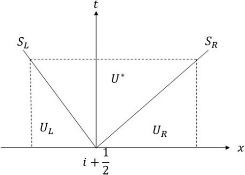
FIGURE 2. Approximate Riemann solver of HLL scheme.
In Figure 2,
where,
The wave velocity algorithm described above is applicable for wet boundaries. For dry and wet mesh boundaries, Da Silva (2017) proposed a corrected model. When the left river bed is dry, the following calculation can be used:
When the right river bed is dry:
After the homogeneous equations were corrected, the total differential Eq. 9 was decomposed, and the estimation step discrete equation of
For
In order to ensure the stability of the numerical scheme, the display algorithm needs to adjust the time step ∆t at each calculation step to reduce the deviation in the propagation of the source term along the characteristic line, thereby ensuring the stability of the algorithm and the accuracy of the numerical solution. The Courant number CFL should satisfy the following condition (LeVeque, 2002):
In this paper, the value of CFL was assumed to be 0.9 to ensure the stability of the algorithm. Step ∆t was calculated as per the following formula:
Flash floods are a type of disaster that can occur suddenly, and not only do they carry small-sized sediments, but they can also carry large-sized sediments, such as pebbles and gravel. This ability to carry large-sized sediments is a unique feature of alpine rivers and the rivers are subjected to long-term coarsening. Large calculation errors will occur if the sediments are assumed to be uniform. Therefore, the calculation of the grouped sediment transport capacity of non-uniform sediments is one of the key issues to be resolved in the mathematical modelling of river sediment. The idea of a grouped sediment model was first proposed by Einstein. Based on Einstein’s initial idea, Misri, Chiodi et al. established and verified a grouped sediment transport model (Misri et al., 1984; Chiodi et al., 2014). In this research study, the sediments were grouped and arranged by particle size, from small to large. The median size of each sediment group was used for detailed calculations.
The sediment settling velocity was used as the basis for the sediment calculation module. Zhang Ruijin’s formula was used in this research study, and the formula is as follows (Tan et al., 2018):
where,
The sediment transport model consists of the sediment transport equation and the river bed deformation equation. The sediments can be divided into bed load and suspended load according to their particle size. The basic equations of the 2D sediment model are as follows:
In the above equations, ω is the deposition velocity, S∗ and S are the suspended load carrying capacity and the suspended load content, respectively; and α is the scouring coefficient. When deposition is obvious, α = 0.25; when scouring and deposition are alternated, α = 0.5; when scouring is obvious, α = 1.
Liu et al. (1991) proposed the Rz number to differentiate the particle sizes of the suspended load and bed load, where:
In the above equation,
The key to calculating the suspended load is to determine the suspended matter content, S, and sediment-carrying capacity, S*, of the river. S was calculated using the finite volume method with a first-order upwind finite volume method. The regions upstream and downstream of the adjacent grids were judged according to the flux in the normal direction of the common grid interface, and the sediment flux at each interface of the grid was calculated. Furthermore, the sediment flux at each interface was integrated at the specified time step to obtain the suspended load content of the grid. This algorithm can unconditionally guarantee the stability of the suspended load content calculations.
There has not been much research on the sediment-carrying capacity of 2D water flow. Therefore, the sediment-carrying capacity of most 2D mathematic models is usually calculated directly using a 1D sediment-carrying capacity formula or a modified formula. Since the suspended load particles are small, the sediment particles were divided into finer groups in the algorithm. The median size of each group of particles is directly used to calculate the sediment-carrying capacity for the suspended load group. The most commonly used formula is the one developed by Zhang Ruijin, which is given below (Tan et al., 2018):
In the above equation, k and m are the empirical constants of the model’s sediment-carrying capacity, which were derived based on the experimental data collected from the Yangtze River, the Yellow River, several reservoirs, and indoor water channels. Hence, the empirical constants have a high degree of universality. Theoretically, Zhang Ruijin’s indexless formula can be coordinated with Bagnold’s energy formula; and by improving Zhang Ruijin’s formula, the comprehensive coefficient
In the above formula,
In flash floods, the finest and coarsest sediments can differ by more than 100 times, resulting in differences of thousands of times for the settling velocity. Therefore, the mathematical model should calculate the sediment-carrying capacity per group. The sediment-carrying capacity needs to be considered in the transport of sediments suspended in the water and the erosion of the river bed. When the sediment-carrying capacity is greater than the sediment content in the water, the bed surface is eroded. The sediment movement should be considered when calculating the erosion sediment-carrying capacity. The sediment can only be scoured when the flood flow rate exceeds the sediment starting velocity. Hence, Eq. 29 can be improved as follows:
In the above formula,
Therefore, the total carrying rate
In the above formula,
The key to solving Eq. 33 is to calculate the effective gradation of the sediment bed, which is affected by many factors. First, the scouring energy remaining in the water is fully distributed along the water depth so the height of suspended sediments that can be scoured is limited. When the sediments cannot be suspended, the scouring energy that exists in the local water body cannot be used for scouring. Hence, the small sediment transport invariant used for scouring should be related to the suspended height of the scoured sediments. Moreover, the effective gradation of the sediment bed is also greatly affected by how the coarse bed sediments conceal the finer sediments, the effective action of the current drag along the sediment bed surface, and the action of the shear stress on the bed surface (Yang et al., 2020).
Based on the above factors, the effective gradation of the sediment bed can be expressed as follows:
In the above formula,
The model utilizes the Mayer-Peter formula to calculate the bed load for particle sizes greater than 0.2 mm and the Sharmov’s formula is used to calculate the bed load when particle sizes are less than 0.2 mm.
The Mayer-Peter formula (Chien and Wan, 1999):
In the formula, G is the relative weight of sediment to water;
According to Sharmov’s formula,
The river bed deformation calculation includes the elevation changes caused by scouring and deposition of bed and suspended matter. Eq. 26 adopts the time forward difference and integrates the spaces in the grid. Next, the Gaussian deformation was calculated as per the following equation:
Namely,
In the equation,
After a large amount of sediment enters an alpine gully with large gradient, the frontal deposition can develop quickly and in retrograde, potentially causing the water level to increase to twice the normal level with clear water. Such a situation can lead to the phenomenon where minor floods can cause great disasters. In this section, the sharp increase in water level that is typical in alpine gullies with large gradient variations and sediment-carrying capacities is reproduced in combination with experiments on physical models and mathematic models. The purpose is to study the laws of sediment transport, investigate how sediments deposit and extend upstream due to changes in the sediment-carrying capacity of the water flow, and to verify the accuracy of the algorithm.
Since alpine gullies are steep upstream and gentle downstream, an experiment was conducted at the State Key Laboratory of Hydraulics and Mountain River Engineering of Sichuan University using a water channel with varying gradients, as shown in Figure 3A. For the water channel, the upstream slope was designed to 5% (length: 3.2 m) and the downstream slope was 2% (length: 3.8 m). Considering that there will be some influence from local mixing after the addition of sediment at the inlet, the effective test section was set to 6.5 m above the water channel outlet. The water channel was made of Plexiglas, with a width of 20 cm and a depth of 30 cm. The upstream water was controlled by a measuring weir, and a self-designed sediment feeding machine was used to add the sediment. The parameters of the mathematical model are shown in Figure 3B and the calculation area was composed of 9,292 triangular meshes. To optimize the drawing effect, the numerical results of this model were drawn as a 2D representation of the water channel with a horizontal scale of 5:1. The upstream flow rate for the experiment was 4.48 L/s; the downstream flow was allowed to discharge freely; the water channel had a rectangular cross-section, with a roughness factor of 0.035; the sediment content at the inlet boundary was 0.343 kg/s, with particle size of 0.5 mm. In the mathematical model, there is no sediment in the water channel before experiment, only the supplement of sediment at the inlet contributed to the change in bed form.
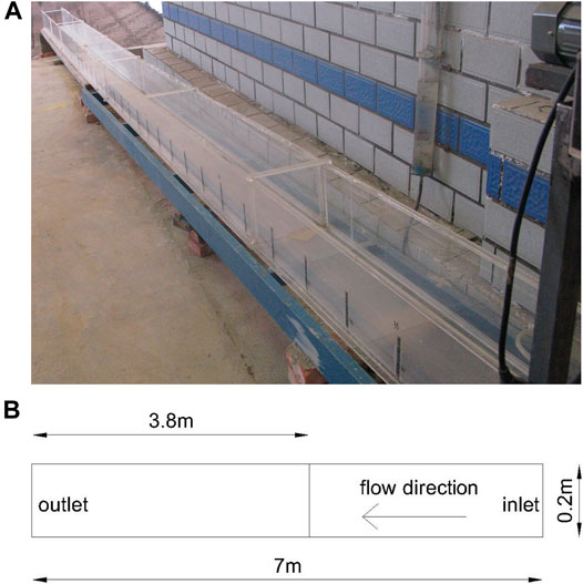
FIGURE 3. (A) Actual image of the variable slope water channel (B) Planar dimensions of the variable slope water channel.
Figure 4 presents the actual images of sediment deposition and water level changes in the physical model experiments. At the beginning of the test, the upstream and downstream water flows at the slope break point were approximately the same as uniform flow, and only the location near the slope break point showed any local changes in water level (Figure 4A). When sediment was added upstream, the sediment-laden water flowed steadily in the steep slope section; however, after entering the downstream section with a slope of 2%, sediment deposits began to form and extend upstream. As the intensity of deposition began to increase, the depth of sediment deposition on the bed surface increased, and the water level at the frontal surface of the deposition increased significantly (Figure 4B). When the deposition extended to the variable slope, the unaffected upstream jet stream velocity was relatively higher, and the hydraulic jumps in the front of the deposition became more obvious (Figure 4C). When the water flow entered the downstream section of the water channel with slope of 5%, the retrograde deposition and increases in water level progressed stably. However, after further retrogradation upstream, the hydraulic jump at the retrograde sediment wave front gradually became unstable, and even resulted in breakage, followed by unsteady fluctuations in the river bed in the frontal section of the retrograde sediment wave (Figure 4D).
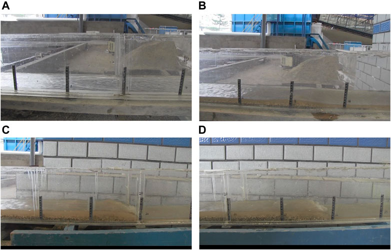
FIGURE 4. Actual images of the physical model at different times: (A) flow state without added sediments; (B) state at the start of deposition (at a slope of 2%); (C) deposition with gradient variations; (D) deposition in the section with 5% slope.
The calculated results from the mathematical model are similar to the experimental results from the physical model. At first, sediment was not added to the upstream inlet until the water flow in the entire water channel became stable. Figure 5 shows a diagram of the water levels produced from the mathematical model when the clear water is at steady-state. When the water flow was clear, the upstream water depth at the slope break point was 0.015 m; the water level at the slope break point increased and gradually stabilized at 0.021 m. Although the water depth in the downstream 2% slope section was larger than that in the upstream, the impact of the backwater did not transmit upstream.
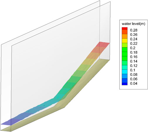
FIGURE 5. Hydrograph of clear water flow.
Figure 6 presents the water level distribution and sediment deposition in the water channel at different times after sediment was added in the channel. After the sediment-laden water left the 5% slope section and entered the 2% slope section, the slope decreased and the sediment deposition caused interference, leading to reductions in water flow energy and flow discharge. Accordingly, the sediment-carrying capacity of the water flow also decreased. When the sediment-carrying capacity was lower than the actual sediment content in the water flow, sediment began to build-up at about 1.8 m behind the slope break point for the first time (Figure 6A). The deposition not only increased the bed resistance but also caused a decrease in the local slope of the bed. The combination of these two effects further reduced the hydraulic conditions of the water flow at the deposition site. When the upstream flow passed through the deposition front, the high flow rate caused the water to flow downstream along the surface of the deposited sandbank. As a result, the actual water level at the deposition location was far higher than the normal water depth of the upstream water flow. Furthermore, sediment from upstream would continue to be deposited here. With the constant deposition at this downstream location, the water level in the local area gradually increased, the water flow energy consumed by the hydraulic jump also increased. The sediment carrying capacity of the water flow was significantly reduced, and serious deposition occurred at the deposition front, and extended upstream continuously. In turn, the hydraulic jumps extended upstream, first reaching the slope break point (Figure 6B) and then the upstream section with slope of 5% (Figure 6C). Due to the high sediment content, deposition occurred at the upstream surface, while the downstream surface was scoured. The sediment scoured in this area was deposited on the upstream surface of the next sediment ridge. As the deposition extended, a continuous retrograde sand dune was formed, causing multiple reverse hydraulic jumps downstream (Figure 6D).
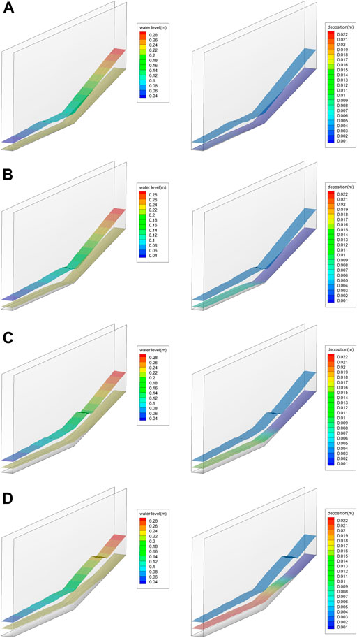
FIGURE 6. Water level distribution (left part) and sediment deposition (right part) at different times: (A) deposition begins; (B) extension to slope break point; (C) extension to the section with slope of 5%; (D) extension to the inlet.
Graphs of the water level and water depth along the central axis of flow are shown in Figure 7. Processes 1–5 in the figure represent the calculated results of the mathematic model at different time. For clear water discharge, the model produced a section of backwater starting from the slope break point, and the water depth was stable at 0.021 m from the from the backwater to a distance of 1.8 m from the outlet. With the addition of sediment, the downstream water depth increased rapidly from the deposition starting point, and dynamic hydraulic jumps gradually appeared and extended upstream. With the continual deposition of sediments on the upstream face, the depth of the dynamic hydraulic jumps increased. The water depth rose from 0.014 m in clear water to 0.029 m when the dynamic hydraulic jump reached 5.8 m from the outlet. As the water depth increased, the water level increased as well due to the continuing deposition of sediments, which aggravated the disaster effect caused by minor flooding.
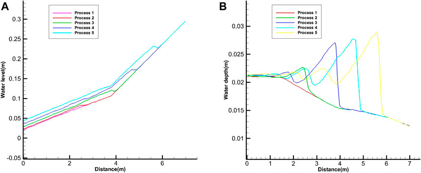
FIGURE 7. Hydraulic factors on the central axis of the water channel at different times: (A) water level; (B) water depth. Processes 1–5 in the figure represent the calculated results of the mathematic model for clear water discharge, start of sediment deposition, and the hydraulic jumps at the slope break point, at the upstream section with 5% slope and in the area near the inlet.
The model results showed that under the action of high-intensity sediment transport and retrograde deposition with large variations in slope, a sharp increase in water depth occurs at each cross section along the gully. In areas unaffected by the retrograde deposition, the water flow state and water depth are also not affected. During deposition, the most drastic changes in water depth occurs at the deposition front, and the increase in water depth is mainly due to the superposition effect of uplift of the river bed caused by sediment deposition on the river bed and the hydraulic jumps in the junction of local rapid and subcritical flow areas. In other words, the relative reduction of power is the premise for the rapid silting up of the river bed, and the frontal surface of deposit forms the basis for subsequent deposition.
On 8 August 2017, heavy rainfall caused a flash flood in Gengdi Village, Liangshan Yi Autonomous Prefecture, Sichuan Province (Figure 8), resulting in 24 deaths. Upstream of the village is a middle mountain area in Yanyuan County, Xichang City, with serious soil erosion. There are two erosion gullies on the mountain, with average longitudinal slope reaching 365%. The right gully, Shaba Gully, abruptly becomes flat after reaching the residential area, causing disasters in the affected area. The left gully, Guangjiahe Gully, is deep and the slope is relatively small, which prevents flood waters from submerging the residential area, avoiding disasters. Due to poor vegetation cover in this area, the heavy rainfall resulted in the convergence of a large amount of sediment entering the gully, and heavy deposition appeared in the left gully, causing water blockage. After the flood waters entered the downstream residential area with the small slope, severe flooding occurred from the small flow in the gully, and the sediment heavy water flowed beyond the protective barriers and submerged the houses, causing a catastrophic flash flood event.
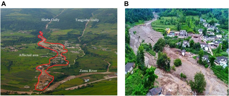
FIGURE 8. Actual images of the flash flood event in Gengdi village: (A) position of the affected area; (B) post-disaster situation in the affected downstream area.
Due to the lack data on the actual flow, water level, and incoming sediment load, the model first forecasted the flow discharge of the two gullies in the disaster area based on the GIUH model, the rainfall data at the actual occurrence place and time of the flash flood, and the DEM data of the local 12 m grid. The time curve of flow discharge at the gully inlet is shown in Figure 9. The inlet of Shaba Gully is 1,840 m away from the disaster area, while that of Tangjiahe Gully is 1,637 m from the disaster area. Zemu River is the outlet, and water flowed freely to the outlet. The DEM data was used to create an irregular grid terrain with a grid length of 4 m, and the number of irregular grids is 210209. Besides, the roughness factor is 0.035 along the gully. The model calculation area is presented in Figure 10. As the DEM terrain data was coarse, the calculation area was larger than the actual drainage area of the gullies. For the hydrodynamic calculations, if the water depth at the grid was less than 0.01 m, it was judged as dry mesh and not included in the calculations. No additional sediment was added at the entrance of the model, and the sediment bed that was formed by the ditch erosion was used as the supply of silt and sand to the disaster area. The gradation of the sediment bed sediment is shown in Table 1.
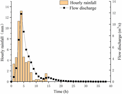
FIGURE 9. Time-lapse curve of flow at the gully inlet.
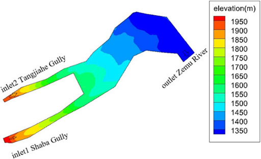
FIGURE 10. Calculation area of the model.

TABLE 1. Sediment Gradation for the Gengdi village flash flood model.
Figure 11 shows the water depth diagram of the disaster area at certain times under the flow duration curve. In the numeric calculations, the rainfall start time was regarded as the starting point, 0 h. At 0 h, the rainfall volume gradually increased and formed a flash flood, which entered the gully inlet and gradually flowed to the disaster area. At 1.5 h, the flash flood was 1 km from the disaster area (Figure 11A). At 2 h, the flood reached Gengdi Village. As the gully slope decreased, the drainage area widened, the flow rate decreased, and sediment began to deposit in the disaster area (Figure 11B). At 2.5 h, the flash flood passed through the entire village. As the rainfall volume continued to increase, and the flow discharge gradually increased as well (Figure 11C). At 4 h, the flow discharge reached a peak and the residential area adjacent to Shaba Gully was submerged. The maximum water depth in the disaster area exceeded 3 m (Figure 11D). After passing through the two gullies, the floods converged at Zemu River.
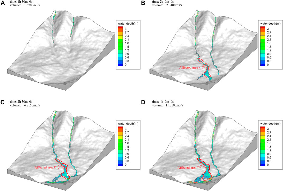
FIGURE 11. Model calculated water levels at different times: (A) 1.5 h; (B) 2 h; (C) 2.5 h; (D) 4 h.
Figure 12 illustrates the water depth and sediment deposition distribution in the affected area of Gengdi Village at 2, 4, 6 and 12 h. It can be seen that during the flash flood, high-intensity sediment transport and the presence of slopes with large gradient variations greatly affected the sediment transport, which aggravated the destructive force of the flood. When the peak flow discharge reached 11.84 m3/s, the flood flowing from Shaba Gully to Gengdi Village passed through an area with gradient variations, from steep slopes to the gentler slopes in the river section. In this area, the flow slowed down, followed by an increase in water level, resulting in a great decrease in the sediment-carrying capacity of the water flow. Sediment rapidly deposited in the gully and enlarged the flooded area. At the flood peak, the water depth in the residential area of the disaster area near the gully exceeded 3 m, with maximum deposition reaching 2.71 m. Due to the sharp increase in water level and heavy sediment content, the houses close to the gully were seriously damaged. In contrast, the Tangjiaba Gully in Gengdi Village is deep and the slope variations are low. Hence, the flood in Tangjiaba Gully flowed closely along the mountain, then downstream to converge with Zemu River. At the flood peak, the maximum water depth and deposition were 1.52 and 0.81 m respectively, which was not enough to extend to the residential area (Figure 12B). With the decrease in rainfall volume during the retreat of the flash flood, the water level in the disaster area decreased gradually, but the deposition continued and reached a maximum of 5.06 m after 12 h. At this time, the gully was filled with sediment (Figure 12D).
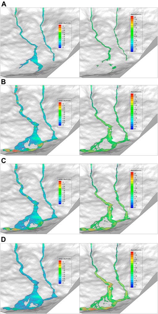
FIGURE 12. Water level distribution (left part) and sediment deposition (right part) in the disaster area at different times: (A) 2 h; (B) 4 h; (C) 6 h; (D) 12 h
In this paper, the finite volume method with Godunov scheme was used to calculate the flow discharge of flash floods in alpine regions with large slope variations, and SGM was used to eliminate the error caused by the source term of the bottom slope. The sediment module was then added over this foundation to explore how the river flow field will change under the action of high-intensity sediment transport and an OPENMP parallel calculation module was incorporated to improve the calculation efficiency. An efficient and accurate flash flood flow and sediment coupling model was established and verified using a generalized experimental model and the actual water level, flow rate and deposition data of the flow field. Finally, the following major conclusions were obtained:
1) Through the physical model experiments and the results from the mathematical model, it was verified that under the action of high-intensity sediment transport, sedimentation will form at the slope break point, leading to an increase in water level and a decrease in the sediment-carrying capacity of the water flow. As a result, sediment quickly accumulated in that location and gradually extended upstream. Eventually the water flow was impacted and hydraulic jumps formed at the interface between rapid and slow flowing waters, causing a sharp increase in water level. Finally, the water depth at the hydraulic jumps near the inlet section increased to more than twice the initial water depth.
2) The flash flood in Gengdi Village was reproduced accurately. Due to the lack of terrain and flow discharge data, a GIUH model was established based on DEM data of a 12 m local grid and the actual rainfall volume during the event to predict the flow discharge in the disaster area and simulate the disaster range and process for average rainfall conditions in the village. The results revealed Shaba Gully experienced a large flooded area, a high amount of sediment deposition and high water levels. The maximum water depth at peak flooding exceeded 3 m, which seriously affected the safety of the residential area.
All the computations were carried out on a workstation equipped with Intel(R) Xeon(R) Platinum 8280 CPU: 28 cores, 56 threads, 2.7 GHz, and 384 GB memory. It cost 40 min of CPU time for 24 h of water and sediment simulation in section 3.2.
The raw data supporting the conclusion of this article will be made available by the authors, without undue reservation.
YD carried out the model simulations and result analysis as well as writing of the manuscript. XL took the leadership of whole project and participated in the discussion and decision-making process. RC developed and tested the numerical code. All the authors participated and contributed to the final manuscript.
This research work was supported by National Natural Science Foundation of China (No. U2040219).
The authors declare that the research was conducted in the absence of any commercial or financial relationships that could be construed as a potential conflict of interest.
All claims expressed in this article are solely those of the authors and do not necessarily represent those of their affiliated organizations, or those of the publisher, the editors and the reviewers. Any product that may be evaluated in this article, or claim that may be made by its manufacturer, is not guaranteed or endorsed by the publisher.
Aizinger, V. (2004). A Discontinuous Galerkin Method for Two-And Three-Dimensional Shallow-Water Equations. Austin, USA: The University of Texas at Austin.
Cao, Z., Pender, G., Wallis, S., and Carling, P. (2004). Computational Dam-Break Hydraulics over Erodible Sediment Bed. J. Hydraul. Eng. 130 (7), 689–703. doi:10.1061/(asce)0733-9429(2004)130:7(689)
Chen, R., Shao, S., and Liu, X. (2015). Water-sediment Flow Modeling for Field Case Studies in Southwest China. Nat. Hazards 78 (2), 1197–1224. doi:10.1007/s11069-015-1765-z
Chiodi, F., Claudin, P., and Andreotti, B. (2014). A Two-phase Flow Model of Sediment Transport: Transition from Bedload to Suspended Load. J. Fluid Mech. 755, 561–581. doi:10.1017/jfm.2014.422
Da Silva, D. A. D. O. (2017). Experimental and Numerical Assessment of Reinforced Concrete Joints Subjected to Shear Loading. Dissertation thesis. (Do Porto(Portugal): Universidade Do Porto.
El Kadi Abderrezzak, K., Paquier, A., and Mignot, E. (2009). Modelling Flash Flood Propagation in Urban Areas Using a Two-Dimensional Numerical Model. Nat. Hazards 50 (3), 433–460. doi:10.1007/s11069-008-9300-0
Guan, M., Wright, N., and Sleigh, P. (2013). “Modelling and Understanding Multiple Roles of Sediment Transport in Floods,” in Proceedings of the 35th IAHR World Congress, Chengdu, China, September 8-13, 2013 (Tsinghua University Press).
Handmer, J. (2001). Improving Flood Warnings in Europe: A Research and Policy Agenda. Glob. Environ. Change B: Environ. Hazards 3 (1), 19–28. doi:10.1016/s1464-2867(01)00010-9
Hapuarachchi, H. A. P., Wang, Q. J., and Pagano, T. C. (2011). A Review of Advances in Flash Flood Forecasting. Hydrol. Process. 25 (18), 2771–2784. doi:10.1002/hyp.8040
Hubbard, M. E., and Dodd, N. (2002). A 2D Numerical Model of Wave Run-Up and Overtopping. Coastal Eng. 47 (1), 1–26. doi:10.1016/s0378-3839(02)00094-7
Hui Pu, J., Shao, S., Huang, Y., and Hussain, K. (2013). Evaluations of SWEs and SPH Numerical Modelling Techniques for Dam Break Flows. Eng. Appl. Comput. Fluid Mech. 7 (4), 544–563. doi:10.1080/19942060.2013.11015492
Juez, C., Murillo, J., and García-Navarro, P. (2013). 2D Simulation of Granular Flow over Irregular Steep Slopes Using Global and Local Coordinates. J. Comput. Phys. 255, 166–204. doi:10.1016/j.jcp.2013.08.002
Kobold, M., and Brilly, M. (2006). The Use of HBV Model for Flash Flood Forecasting. Nat. Hazards Earth Syst. Sci. 6 (3), 407–417. doi:10.5194/nhess-6-407-2006
Lane, E. W., and Kalinske, A. A. (1941). Engineering Calculations of Suspended Sediment. Trans. AGU 22 (3), 603–607. doi:10.1029/tr022i003p00603
LeVeque, R. J. (2002). Finite Volume Methods for Hyperbolic Problems. Cambridge, UK: Cambridge University Press.
Li, Wei. (2006). Roe-Upwind Finite Volume Model and Numerical Simulation of Hydrodynamic Mechanism of Tidal Bore. Dissertation Thesis. Nanjing: Hohai University.
Liang, Q., Xia, X., and Hou, J. (2016). Catchment-scale High-Resolution Flash Flood Simulation Using the GPU-Based Technology. Proced. Eng. 154, 975–981. doi:10.1016/j.proeng.2016.07.585
Liu, X., Zhou, Q., Huang, S., Guo, Y., and Liu, C. (2018). Estimation of Flow Direction in Meandering Compound Channels. J. Hydrol. 556, 143–153. doi:10.1016/j.jhydrol.2017.10.071
Liu, X., Chen, Y., and Chen, J. (1991). Study of the Distribution of Total Sediment Concentration. Prog. Nat. Sci. Commun. State. Key Laboratories China (Chinese) 05, 405–414.
Ministry of water resources of the people’s republic of China (2018). Bulletin on Flood and Drought Disasters in China of 2018. Available at: http://www.mwr.gov.cn/sj/tjgb/zgshzhgb/ (Accessed July, , 2019).
Misri, R. L., Garde, R. J., and Ranga Raju, K. G. (1984). Bed Load Transport of Coarse Nonuniform Sediment. J. Hydraulic Eng. 110 (3), 312–328. doi:10.1061/(asce)0733-9429(1984)110:3(312)
Norbiato, D., Borga, M., Sangati, M., and Zanon, F. (2007). Regional Frequency Analysis of Extreme Precipitation in the Eastern Italian Alps and the August 29, 2003 Flash Flood. J. Hydrol. -Amsterdam- 345 (3-4), 149–166. doi:10.1016/j.jhydrol.2007.07.009
Om, S. B. (1976). Development and Application of a Conceptual Runoff Model for Scandinavian Catchments. Report RH07.
Penning-Rowsell, E. C., Tunstall, S. M., Tapsell, S. M., and Parker, D. J. (2000). The Benefits of Flood Warnings: Real but Elusive, and Politically Significant. Water Environ. J 14 (1), 7–14. doi:10.1111/j.1747-6593.2000.tb00219.x
Piotrowski, A., Napiórkowski, J. J., and Rowiński, P. M. (2006). Flash-flood Forecasting by Means of Neural Networks and Nearest Neighbour Approach - A Comparative Study. Nonlin. Process. Geophys. 13 (4), 443–448. doi:10.5194/npg-13-443-2006
Pu, J. H., Cheng, N.-S., Tan, S. K., and Shao, S. (2012). Source Term Treatment of SWEs Using Surface Gradient Upwind Method. J. hydraulic Res. 50 (2), 145–153. doi:10.1080/00221686.2011.649838
Pu, J. H., Hussain, K., Shao, S.-d., and Huang, Y.-f. (2014). Shallow Sediment Transport Flow Computation Using Time-Varying Sediment Adaptation Length. Int. J. Sediment Res. 29 (2), 171–183. doi:10.1016/s1001-6279(14)60033-0
Reid, I., Laronne, J. B., and Powell, D. M. (1998). Flash-flood and Bedload Dynamics of Desert Gravel-Bed Streams. Hydrol. Process. 12 (4), 543–557. doi:10.1002/(sici)1099-1085(19980330)12:4<543:aid-hyp593>3.0.co;2-c
Roca, M., Martín-Vide, J., and Moreta, P. (2009). Modelling a Torrential Event in a River confluence. J. Hydrol. 364 (3-4), 207–215. doi:10.1016/j.jhydrol.2008.10.020
Roe, P. L. (1997). Approximate Riemann Solvers, Parameter Vectors, and Difference Schemes. J. Comput. Phys. 135 (2), 250–258. doi:10.1006/jcph.1997.5705
Shan, Y., Huang, S., Liu, C., Guo, Y., and Yang, K. (2018). Prediction of the Depth-Averaged Two-Dimensional Flow Direction along a Meander in Compound Channels. J. Hydrol. 565, 318–330. doi:10.1016/j.jhydrol.2018.08.004
Sirdaş, S., and Şen, Z. (2007). Determination of Flash Floods in Western Arabian Peninsula. J. Hydrologic Eng. 12 (6), 676–681. doi:10.1061/(ASCE)1084-0699(2007)12:6(676)
Tan, G., Fang, H., Dey, S., and Wu, W. (2018). Rui-Jin Zhang's Research on Sediment Transport. J. Hydraul. Eng. 144 (6), 02518002. doi:10.1061/(asce)hy.1943-7900.0001464
Toro, E. F. (1992). Riemann Problems and the WAF Method for Solving the Two-Dimensional Shallow Water Equations. Phil. Trans. R. Soc. Lond. Ser. A: Phys. Eng. Sci. 338 (1649), 43–68. doi:10.1098/rsta.1992.0002
Wang, X., Cao, Z., and Tan, G. (2009). Shallow Water Hydrodynamic Modelling of Rainfall Induced Flash Flooding. Eng. J. Wuhan Univ. 42 (4), 413–416.
Weishuai, C. (2013). A Review of Rainfall Thresholds for Triggering Flash Floods. Adv. Water Sci. (Chinese) 24 (6), 901–908. doi:10.14042/j.cnki.32.1309.2013.06.012
Wu, W., Wang, S. S. Y., and Jia, Y. (2000). Nonuniform Sediment Transport in Alluvial Rivers. J. hydraulic Res. 38 (6), 427–434. doi:10.1080/00221680009498296
Yang, F., Ni, Y., Huang, W., and Liu, J. (2020). Numerical Modelling of Dam-Break Floods in Chushandian Reservoir. Yellow River 42 (1), 27–36. doi:10.3969/j.issn.1000-1379.2020.01.006
Yuntian, S., Xin, Z., Yu, Z., Chenge, A., Meihong, M., and Xudong, F. (2019). Effect of Sediment Transport on the Temporal and Spatial Characteristics of Flash Floods: A Case Study of “7.21” Flood in Beijing. J. Tsinghua Univ. (Science Technology) 59 (12), 990–998. doi:10.16511/j.cnki.qhdxxb.2019.26.023
Zheng, X.-g., Chen, R.-d., Luo, M., Kazemi, E., and Liu, X.-n. (2019). Dynamic Hydraulic Jump and Retrograde Sedimentation in an Open Channel Induced by Sediment Supply: Experimental Study and SPH Simulation. J. Mt. Sci. 16 (8), 1913–1927. doi:10.1007/s11629-019-5397-8
Keywords: flash flood, high-intensity sediment transport, 2D flow and sediment simulation, gully with large gradient variations, Gengdi village
Citation: Ding Y, Liu X and Chen R (2022) Numerical Simulation of Alpine Flash Flood Flow and Sedimentation in Gullies With Large Gradient Variations. Front. Environ. Sci. 10:858692. doi: 10.3389/fenvs.2022.858692
Received: 20 January 2022; Accepted: 31 January 2022;
Published: 01 March 2022.
Edited by:
Jaan H. Pu, University of Bradford, United KingdomReviewed by:
Jiarui Lei, National University of Singapore, SingaporeCopyright © 2022 Ding, Liu and Chen. This is an open-access article distributed under the terms of the Creative Commons Attribution License (CC BY). The use, distribution or reproduction in other forums is permitted, provided the original author(s) and the copyright owner(s) are credited and that the original publication in this journal is cited, in accordance with accepted academic practice. No use, distribution or reproduction is permitted which does not comply with these terms.
*Correspondence: Ridong Chen, Y2hlbnJpZG9uZzE5ODRAMTYzLmNvbQ==
Disclaimer: All claims expressed in this article are solely those of the authors and do not necessarily represent those of their affiliated organizations, or those of the publisher, the editors and the reviewers. Any product that may be evaluated in this article or claim that may be made by its manufacturer is not guaranteed or endorsed by the publisher.
Research integrity at Frontiers
Learn more about the work of our research integrity team to safeguard the quality of each article we publish.