Multi-Temporal Landslide Inventory-Based Statistical Susceptibility Modeling Associated With the 2017 Mw 6.5 Jiuzhaigou Earthquake, Sichuan, China

The 2017 M_w 6.5 Jiuzhaigou earthquake (Sichuan, China) is the first strong ground motion that struck the famous world heritage site, causing widespread landslides and severe rock mass damage effects and landscapes undergoing rapid evolution in the Jiuzhaigou National Geopark. However, the understanding of the variability of pre- and post-earthquake landslide susceptibility and landslide conditioning factor effects over time remains limited. This study aims to carry out multi-temporal statistical landslide susceptibility modeling at the slope-unit level related to this event. To achieve this, we initially used a set of remote sensing imageries in GIS to obtain systematic landslide inventories across the pre-, co-, and post-seismic periods. Based on three landslide inventory datasets, we developed three statistical models by incorporating 14 landslide conditioning (seismic, topographic, and geologic) factors into a binary logistic regression (BLR) model. Finally, we utilized the area under the receiver operating characteristic (AUC) (QA) curve to assess each model’s calibration and validation performance. The results show that the BLR model has good prediction applicability for both normal and seismic landslides in the study area with outstanding to excellent predictive accuracy for Mod1 (pre-seismic, AUC = 0.801), Mod2 (co-seismic, AUC = 0.942), and Mod3 (post-seismic, AUC = 0.880) periods. There are variations in both the importance of landslide conditioning factors and susceptibility maps through time, and the number of slope units with a mean probability over 0.8 from only one (pre-seismic) increased to 21 (post-seismic). The dynamic susceptibility maps are of great significance for identifying potentially unstable slopes and providing references for hazard and risk assessment, which could provide new insights into geo-environmental protection and regional landslide evaluation in scenery spots, even for those world heritage sites in the tectonic active mountainous region. Moreover, more frequent or extended observation periods could contribute a further understanding of the post-seismic landslide developments in the Jiuzhaigou area.

Highlights

◆ Statistical landslide susceptibility space–time modeling at the slope-unit level for a world heritage site was carried out.

◆ The multi-temporal landslide inventory datasets (154 pre-, 1022 co-, and 364 post-seismic periods) related to the 2017 Jiuzhaigou earthquake (M_w = 6.5) were obtained.

◆ There are variations in both landslide susceptibility and conditioning factors’ effects over time.

Introduction

The likelihood of the landslide occurrence in a given area based on a set of slope failure conditioning factors is known as landslide susceptibility (Brabb, 1985; Varnes, 1984), and it can be obtained through different approaches and mapping units (Carrara et al., 1995; Guzzetti et al., 1999). The landslide research community has conducted a vast number of landslide susceptibility assessment studies over the past 3 decades, especially through four groups of approaches and methods: 1) Heuristic (knowledge-based) methods (Van Westen et al., 2003); 2) Deterministic (physically based) methods (e.g., Guzzetti et al., 1999; Montgomery and Dietrich, 1994; Newmark, 1965; Van Westen et al., 2003); 3) Data-driven methods, including statistical methods, such as logistic regression, frequency ratio, certainty factor, statistical index, and weight of evidence models (Brenning, 2005; Reichenbach et al., 2018), and machine learning techniques (e.g., Micheletti et al., 2014; He and Kusiak, 2017; Li et al., 2021a, Li et al., 2021b); and 4) innovative combination of these methods (e.g., Chen et al., 2017; Strauch et al., 2019; Zhou et al., 2021). Among the aforementioned techniques, data-driven models were most frequently chosen in the recent past and characterized as objective and practical and were proven valuable and robust (Brenning, 2005; Reichenbach et al., 2018). Effective landslide susceptibility mapping plays a vital role in risk assessment and mitigation and could also provide land and infrastructure management for planners (Guzzetti et al., 2006; Fell et al., 2008).

It is generally recognized that the assumption “future landslides will be more likely to occur under the conditions which led to the landslides past and present” is at the base of statistical landslide susceptibility modeling (Varnes, 1984; Furlani and Ninfo, 2015; Samia et al., 2017). In this regard, the susceptibility maps for a given area can be considered to be static (Segoni et al., 2018). This notion may hold true for non-seismically caused landslides during a short period. However, earthquake-induced landslide analyses are inevitably much more complex, compared to the naturally occurring slope instability (Nowicki et al., 2014; Nowicki Jessee et al., 2018). A strong earthquake could not only trigger a large amount of co-seismic landslides but also drastically deteriorate the rock and soil physical and mechanical properties. As a result, seismic-affected quasi-stable cracked slopes are prone to be unstable during subsequent rainfall, resulting in increased landslide activity and impacts compared to the pre-earthquake period (Huang and Li, 2014). The long-term effects of the regional landslide susceptibility over annual to decadal timescales, which peaks immediately after a major earthquake, remains high for several months to years and even decades, and then falls to the background susceptibility level, were highlighted by Fan et al. (2019b). Lin et al. (2006) found the intensity of seismic-induced landslides was the highest in the first 5 years after the Chi-Chi earthquake and then showed a decreasing trend year by year. In that case, the long-term effects could lead to considerable and severe loss of lives and property in mountainous and tectonic-active areas (Keefer, 1984, Keefer, 2002; Fan et al., 2019b), and it is necessary to track the response of slopes to a landslide for a significant period after the earthquake (Khattak et al., 2010).

To date, co-seismic landslide susceptibility assessments have been carried out worldwide for single events, particularly those caused by catastrophic earthquakes (Lee et al., 2008; Kamp et al., 2008; Xu et al., 2012; Shrestha and Kang, 2019; Cui et al., 2021). Compared to the single event-based inventory, the multi-temporal inventory represents the optimal landslide information for 1) producing reliable susceptibility maps (Galli et al., 2008) and 2) testing the long-term performances of a susceptibility model (Guzzetti et al., 2006). In fact, there has been a surge in interest in the temporal evolution of landslides after major earthquakes in recent decades, particularly since the 1999 Chi-Chi, the 2008 Wenchuan, and the 2015 Gorkha earthquakes (Marc et al., 2015; Tang et al., 2016; Yang et al., 2017; Fan et al., 2018a, Fan et al., 2019a; Kincey et al., 2021). Few studies have been devoted to the multi-temporal landslide evolution and time-relevant susceptibility assessment. For instance, Fan et al. (2021) exploited a multi-temporal inventory (2005–2018) spanning the epicentral region of the Wenchuan earthquake and a random forest model to model the landslide susceptibility. By applying the binary logistic regression model and analyzing the time series of landslides related to four earthquakes in Indonesia, Tanyas et al. (2021a) and Tanyas et al. (2021b) studied the coupled influence of earthquakes and rainfall to predict landslide occurrences. These studies are pioneer attempts on the spatial-temporal variation and dynamic susceptibility/hazard of post-seismic landslides in an earthquake-affected area.

On 8 August 2017, the Jiuzhaigou earthquake with a magnitude of M_w 6.5 struck the 76 Jiuzhaigou county, northern Sichuan province, China. The epicenter is within the Jiuzhaigou National Geopark, a famous world heritage site certified by the United Nations Educational, Scientific, and Cultural Organization (UNESCO). This event triggered a significant amount of co-seismic landslides, and touristic infrastructures were seriously damaged (Wang et al., 2018). After this event, substantial studies were published, most of which focused on the co-seismic landslide spatial distribution analysis (Fan et al., 2018b; Wang et al., 2018; Wu et al., 2018; Tian et al., 2019; Chen et al., 2020; Ling et al., 2021) and susceptibility/hazard assessment (Fan et al., 2018b; Ma et al., 2019; Yi et al., 2019; Cao et al., 2020), which could be useful in the emergency response phase. Despite the rapid evolution of landscapes as a result of earthquake-induced rock mass damage and three extremely heavy rainfall events in September 2017, August 2018, and August 2019 (Hu et al., 2019), assessing the dynamic landslide susceptibility in the years following the mainshock has rarely been performed. Guo et al. (2021) used remote sensing data to monitor the spatio-temporal characteristics of landslides and how they changed after the Jiuzhaigou earthquake. Preparing dynamic susceptibility maps is important, which can help us better understand the evolution of landslides and assist geo-hazard reduction and risk management. For this purpose, this work selected the Jiuzhaigou National Geopark as the study region and utilized the binary logistic regression model at the slope-unit level to conduct a case study on the spatial patterns of pre-, co-, and post-seismic landslide susceptibility, as well as the covariates’ effect over time. This research may enrich the theoretical research content of post-earthquake landslide regional assessment and provide references for disaster prevention and mitigation for the scenery spot in tectonic-active mountainous areas.

Study Area

The study area, a UNESCO world heritage site known as the Jiuzhaigou National Geopark, is situated in the eastern edge of the Tibetan Plateau. The site with an area of approximately 653 km² is located at 32°54′21″ ∼33°16′9″ N and 103°46′24″∼104°3′54″ E in the northern part of Sichuan province, southwestern China (see Figure 1A). It is a tectonically active hilly mountainous region characterized by narrow and steep valleys with elevations ranging from 1429 to 4865 m a.s.l. (above the sea level). The annual precipitation in the region is about 704.3 mm and peaks from June to September, accounting for approximately 70% of the yearly precipitation. This region lies between two principal faults: the nearly NS-trending Minjiang Fault and the NWW-trending left-lateral strike-slip Tazang Fault (Fan et al., 2018b; Wu et al., 2018) (Figure 1B). All of these active structures have the potential for triggering earthquakes of magnitude M_L ≥ 7.5 (Li et al., 2016). According to historical earthquake records, this region was affected by seven strong earthquake events in the last century, including the 1933 Diexi M_w 7.3 earthquake, 1960 Songpan M_w 6.3 earthquake, 1973 Songpan M_w 6.1 earthquake, 1974 Songpan M_w 5.7 earthquake, and 1976 Songpan–Pingwu earthquake swarm (M_w 6.9 occurred on 16 August, M_w 6.4 on 21 August, and M_w 6.7 on 23 August) (see Figure 2 in Luo et al., 2021). These events may have caused serious damage to the rock masses, increasing the probability of slope failure. More specific information about the study area can be found in the studies by Luo et al. (2021) and Wang et al. (2018), as well as references therein.

FIGURE 1

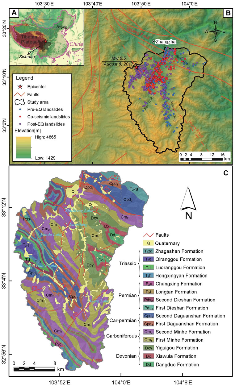
FIGURE 1. (A) Geographical location map of the study area in southwestern China; (B) Regional tectonic setting, epicenter, and distribution of multi-temporal landslide identification points (LIPs) within the Jiuzhaigou National Geopark. EQ stands for the 2017 M_w 6.5 Jiuzhaigou earthquake; (C) Geologic map showing the outcropping lithology and fault lines of the study area. F1: Ergen Fault, F2: Zharugou Fault, F3: Heye Fault, F4: Luweihai Fault, F5: Zechawa Fault, F6: Jiuzhaigou Fault, F7: Yingzhuadong Fault, F8: Xuanquan Fault, F9: Loubangou Fault, and F10: Changhai Fault.

FIGURE 2

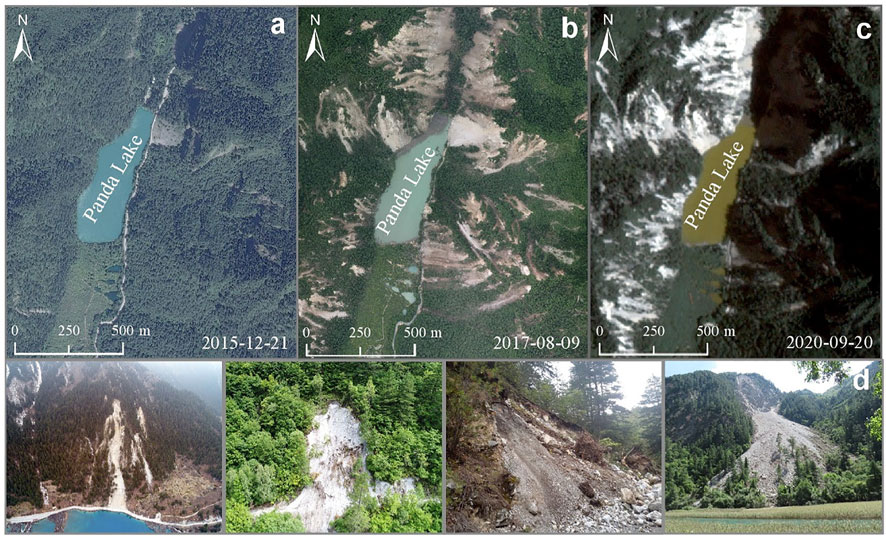
FIGURE 2. (A) Pre-earthquake, (B) co-seismic, and (C) post-seismic satellite images around Panda Lake for multi-temporal landslide interpretation; (D) Photographs obtained from the field surveys showing typical landslides in the study area.

The geological map at a scale of 1:50,000 was provided by the Jiuzhaigou Management Bureau and modified from the published research studies (Cui et al., 2005; Hu et al., 2019). Outcrops in the study area can be grouped into 16 lithological units, and loose Quaternary materials locally covered the Triassic (T), Permian (P), Carboniferous–Permian (Cp), Carboniferous(C), and Devonian(D) rocks (see Table 1 and Figure 1C).

TABLE 1

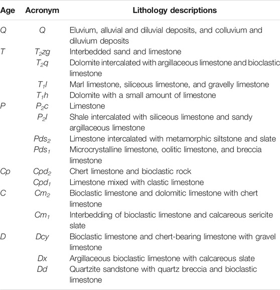
TABLE 1. Description of geologic units and lithology of the study area.

Method and Materials

Multi-Temporal Landslide Inventory

It is a crucial pre-requisite phase to build a trustworthy and accurate landslide inventory map for landslide analysis (Guzzetti et al., 1999; Li et al., 2022; Tanyas and Lombardo, 2020). In this study, the imagery for interpretation was chosen based on the year of acquisition, coverage, minimum of clouds, and resolution to detect multi-temporal landslides. In particular, for co-seismic landslides, it is rather necessary to collect the pre-seismic images that are closer to the earthquake event occurrence date in order to exclude the pre-earthquake landslides and misjudged zones (Harp et al., 2011). This study mapped multi-temporal landslides via a set of remote sensing images from Spot-5, Gaofen, Landsat, unmanned aerial vehicle (UAV), and Google Earth platform, followed by field investigation for the temporal span from August 2017 to September 2020. The spatial resolutions of images range from 0.2 to 3.0 m. We refined landslide signatures through the systematic visual interpretation in the geographic information system (GIS) environment. Table 2 summarizes the sources and characteristics of data used for landslide interpretation and susceptibility modeling phases. Satellite images around Panda Lake used for multi-temporal landslide identification and some typical landslide photographs in the study area are shown in Figure 2.

TABLE 2

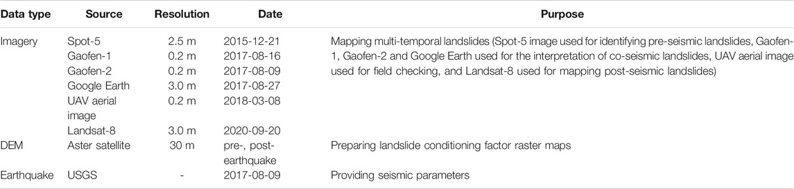
TABLE 2. The type, source, and date of the data used for landslide mapping and the subsequent modeling procedure. USGS represents the U.S. Geologic Survey.

As a result, we created detailed polygon-shaped multi-temporal landslide maps that record the location, surface area, and types of pre-, co-, and post-seismic landslides. Unfortunately, landslide initiations were not separated from the runout and deposition areas. In general, it requires conducting a polygon-to-point conversion for each landslide to build a statistical susceptibility assessment model. Previous studies offer three categories of sampling strategies (Hussin et al., 2016), and extracting the points populating the scar on a buffer distance is a common choice. Specifically, we first extracted the highest and lowest elevations of each landslide polygon and then calculated the 20% of the height difference as the buffer distance to the most elevated location of the scar, producing landslide identification points (LIPs, as shown in Figure 1B). The types of landslides are mainly small-medium scale shallow debris/rock slides, rock avalanches, and rockfalls (Hungr et al., 2014).

The size distribution and morphometric characteristics of the mapped landslides are illustrated in Figure 3. The pre-EQ landslide dataset contains landslides covering an area of 3.83 × 106 m² in total, and the size varied from A_Lmin = 940.94 m² to A_Lmax = 30.98 × 104 m² (µ = 2.49 × 104 m², σ = 4.24 × 104 m², see Figure 3A), spanning the scale from small to moderate. Subsequently, we mapped 1022 co-seismic landslides with a total covering area of 3.88 × 106 m², ranging in size from A_Lmin = 10.21 m² to A_Lmax = 6.47 × 104 m² (µ = 0.37 × 104 m², σ = 0.62 × 104 m², Figure 3B). The 364 landslides (post-EQ, covering an area of 2.11 × 106 m²) range in size from 3.89 × 102 m² to 5.39 × 104 m² (µ = 0.58 × 104 m², σ = 0.62 × 104 m², Figure 3C) after the earthquake occurred to the present. Subsequently, for each landslide dataset, we generated a corresponding temporal model with a set of covariates in the Binary Logistic Regression Model.

FIGURE 3

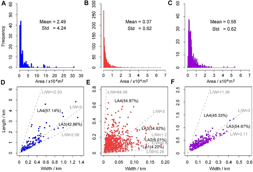
FIGURE 3. Morphometric characteristics of the mapped landslides: the frequency distribution histogram of the landslide area and the scatter plot showing the aspect ratio (L/W) for (A,D) pre-EQ landslides; (B,E) co-seismic landslides; and (C,F) post-EQ landslides, respectively.

The aspect ratio (also called the length–width ratio, L/W) describes the planar shape of a single landslide (Tian et al., 2017). According to values of this parameter, the landslides were categorized as 1) the transverse landslide (LA1, L/W ≤ 0.8), 2) the isometric landslide (LA2, 0.8 < L/W ≤ 1.2), 3) the longitudinal landslide (LA3, 1.2 < L/W ≤ 3), and 4) the elongated landslide (LA4, L/W > 3). An aspect ratio close to 1 means a typical rotational slide, and with the increase of the aspect ratio, it is a much more elongated shape typical of flow-type landslides. According to the statistics, the minimum and maximum aspect ratios for pre-EQ landslides (Figure 3D), co-seismic landslides (Figure 3E), and post-EQ landslides (Figure 3F) are 2.09, 0.29, and 2.11 and 12.03, 84.08, and 11.36, respectively. The average value equals 3.66, 5.04, and 3.34, respectively. Moreover, it is similar that all landslides for three datasets are mainly composed of longitudinal (LA3) and elongated landslides (LA4). Specifically, LA3 accounted for 42.86%, 34.92%, and 54.67% and LA4 for 57.14%, 54.87%, and 45.33% for pre-, co-, and post-seismic landslides, respectively. This elongation resulted, in general, from moderately long run-out distances down steep slopes below landslide source areas.

Slope Units Delineation and Status Assignment

In the vast literature reports (e.g., Carrara et al., 1995; Guzzetti et al., 1999; Reichenbach et al., 2018), the most frequent mapping units for large-scale or regional landslide susceptibility assessments are grid cells and slope units (SUs, hereafter). SUs are the basic units of landslide occurrence generated according to the terrain hydrology unit bounded by drainage and ridgelines (Carrara et al., 1995). Compared to the grid cells, SUs offered two main advantages: one for a smaller computational burden and the other for the geomorphologically oriented interpretation (Steger et al., 2016). Because it has higher internal homogeneity and between-unit heterogeneity, SUs have been proven to be reliable, as tested in some cases by Alvioli et al. (2016), Amato et al. (2019), and Lombardo et al. (2020). In this study, the r.slopeunits module (Alvioli et al., 2016) was used to automatically delineate SUs from an input DEM, and the study area was partitioned into 1234 SUs. Figure 4A portrays the size distribution and statistic characteristics of the generated slope-units. Their areas range from a minimum of 0.05 km² to a maximum of 3.25 km² with a mean of 0.53 km², and a standard deviation 0.43 km², indicating that the local topography is fairly rugged.

FIGURE 4

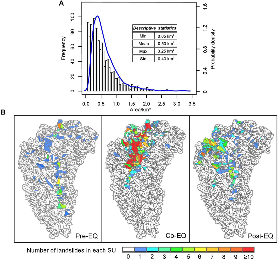
FIGURE 4. (A) The size distribution and geometric features of partitioned 1234 SUs; (B) Delineation, landslide intensity, and the presence–absence status assignment of partitioned SUs in the study area associated with pre-, co-, and post-EQ landslides.

For each landslide inventory, we counted the LIPs per SU and transformed the results to binary presence–absence to reflect the presence–absence of the landslide distribution over the study area at the SU level. If an SU included at least one LIP, it was given a positive landslide status of “1,” and if not, it was set as “0” for an absence status. The presence/absence status assignment of the partitioned 1234 SUs for each landslide inventory is shown in Figure 4B. Consequently, 96 SUs (i.e., ∼ 7.78% of the total 1234 SUs) were assigned as “1,” while the remaining 1138 SUs were allocated as “0” for the pre-EQ landslide dataset. Regarding the co-seismic landslide inventory, 173 SUs accounting for approximately 14.02% of the total SUs were classified as presence, while the rest were classified as absence, which accounts for 86% of all SUs. For the post-EQ landslides, 163 SUs were assigned as “1,” accounting for 13.21% of the total (N = 1234) SUs.

Binary Logistic Regression Model

In this work, we opted for a probabilistic model as the binary formulation of the logistic regression model. It is a generalized linear model belonging to the statistical family and widely used in the vast majority of slope failure studies for a given mapping unit to explain the distribution of landslides over space (Brenning, 2005; Reichenbach et al., 2018). More specifically, it aims at modeling a linear relationship between covariates and landslide occurrences based on a set of predictors, which can correspond either to continuous or categorical variables in the model. The BLR model assumes a Bernoulli probability distribution as the underlying stochastic process, and it can be stated as follows:pt

$\mathit{\eta }\left(\mathit{x}\right)=\mathbf{In}\left[\frac{\mathit{\pi }\left(\mathit{x}\right)}{1-\mathit{\pi }\left(\mathit{x}\right)}\right]={\mathit{\beta }}_0+{\mathit{\beta }}_1{\mathit{x}}_1+\cdots +{\mathit{\beta }}_{\mathit{j}}{\mathit{x}}_{\mathit{j}},(1)$

where η is the logic link, π(x) is the conditional probability of the landslide occurrence, given the predictors, β₀ is the constant intercept, and β₀, … …, β_j are regression coefficients measuring the effects of each covariate. Once the model has estimated the linear predictor, the following logic link η is used to obtain the probability of the landslide occurrence P:

$\mathit{P}=\frac{{\mathit{e}}^{{\mathit{\beta }}_0+{\mathit{\beta }}_1{\mathit{x}}_1+\cdots +{\mathit{\beta }}_{\mathit{j}}{\mathit{x}}_{\mathit{j}}}}{1+{\mathit{e}}^{{\mathit{\beta }}_0+{\mathit{\beta }}_1{\mathit{x}}_1+\cdots +{\mathit{\beta }}_{\mathit{j}}{\mathit{x}}_{\mathit{j}}}}.(2)$

Covariates and Multi-Collinearity Analyses

Covariates

Because of the complexity of the nature and evolution of landslides, there is no standard guideline on which causative factors should be included in the landslide susceptibility assessment model. Based on the literature review of other earthquake cases (e.g., Nowicki et al., 2014; Tanyas et al., 2021a; Fan et al., 2021), the same area (Fan et al., 2018b; Tian et al., 2019; Yi et al., 2019; Luo et al., 2021), and data availability and reliability for the study area, we considered 14 conditioning factors to explain the spatial distribution of pre-, co-, and post-seismic landslides. Rainfall was not chosen due to the restricted variety of precipitation in our study area. Ultimately, these factors are elevation (EL), slope angle (SL), northness (NN), eastness (EN), planar curvature (PLC), profile curvature (PRC), relative slope position (RSP), topographic wetness index (TWI), distance to roads (Dis2roads), distance to rivers (Dis2rivers), distance to faults (Dis2faults, see faultlines in Figure 1C), lithology, peak ground acceleration (PGA), and distance to the seismogenic fault (Dis2seisfaults). For each continuous factor, the mean (µ) and standard deviation (σ) values from the normal distribution per SU were further aggregated and computed as covariates (Guzzetti et al., 2006). In terms of lithology, we extracted the most represented class in each slope-unit. Table 3 summarizes the full list of these causative factors and their properties, which are then displayed in Figure 5.

TABLE 3

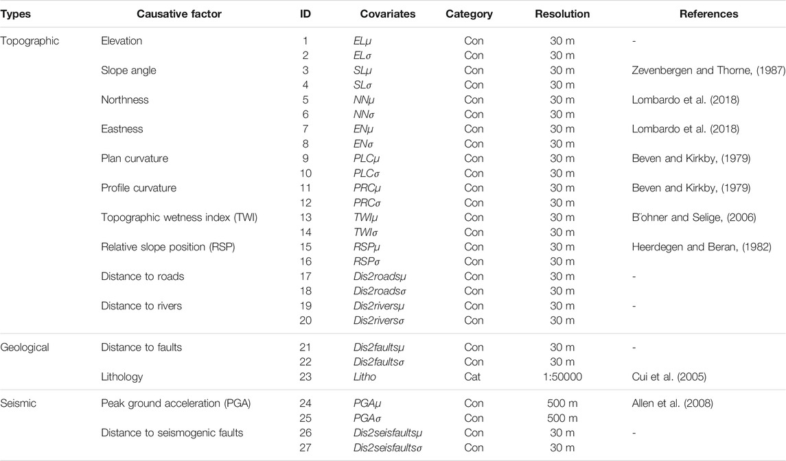
TABLE 3. List of topographic, geologic, and seismic factors in the study area for the subsequent modeling procedure. Con or Cat indicates the continuous or categorical nature of the covariates.

FIGURE 5

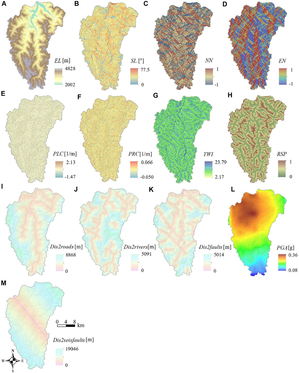
FIGURE 5. Spatial distribution of conditioning factor raster layers in the grid used for modeling phases in the study area: (A) Elevation, (B) Slope angle, (C) Northness, (D) Eastness, (E) Plan curvature, (F) Profile curvature, (G) TWI, (H) RSP, (I) Distance to roads, (J) Distance to rivers, (K) Distance to faults, (L) PGA, and (M) Distance to seismogenic faults.

A 30 m spatial resolution digital elevation model (DEM) was used to extract the topographic parameters. The elevation ranges from 2002 to 4828 m a.s.l. (Figure 5A), and the slope angle ranges between 0 and 77.5° (Figure 5B). The slope aspect was transformed according to the study by Lombardo et al. (2018) into two linear continuous covariates: northness (NN, Figure 5C) and eastness (EN, Figure 5D), both of which range between −1 and 1. Additionally, PLC, PRC, TWI, and RSP (Figures 5E–H) were obtained. We computed the Euclidean distance to the nearest roadways (Figure 5I) and rivers (Figure 5J) to account for both anthropogenic and hydrology effects. Lithology and faults were derived by vectorization of 1:50,000 geologic maps (see Figure 1C and Table 1). Similarly, we computed the distance to faultlines (Dis2faults, Figure 5K), following the same operation with roadways and streamlines. The seismic factors used in this research include PGA (see Figure 5L) and Dis2seisfaults (Figure 5M). The PGA of the Jiuzhaigou earthquake was available on the website of the USGS (https://earthquake.usgs.gov/earthquakes/eventpage/us2000a5x1/impact) and then digitalized into raster; the pattern shows a generally southward decrease of PGA levels from 0.36 to 0.08 g, with the distance far away from the epicenter. Besides, we computed the distance to the causative faults (northwest section of the Huya fault according to Fan et al. (2018b) and Yi et al. (2018)). Ultimately, we rasterized all the vector layers into corresponding 30 m resolution layers to support subsequent analyses.

Notably, the explanatory covariates for multi-temporal landslide susceptibility models (pre-seismic Mod1, co-seismic Mod2, and post-seismic Mod3) are pretty different with the drift of time. Due to the ground shaking damage effects on the rock masses, the post-seismic landslide susceptibility assessment should also consider the seismic parameters. Therefore, all these covariates in Table 3 were incorporated into Mod2 and Mod3 shared, whereas pre-seismic Mod1 removed these seismic covariates.

Multi-Collinearity Test for Covariates

The large covariates’ hyperspace we have built may posess the potential multi-collinearity issue, which would have a negative impact on our statistical models (Kelava et al., 2008). To avoid this, we performed a multi-collinearity test and utilized Pearson’s correlation coefficients r to measure how closely the variables are linearly related. In accordance to Moore et al. (2006), |r| ≤ 0.8 stands for an extremely weak collinearity that can be considered with barely no linear dependency between the pairs of covariates. Figure 6 is the Pearson’s correlation coefficient matrix obtained in the software R. Overall, not even one case exceeded the thresholds (|r| = 0.8) for significant dependency although some moderate pair-wises existed, including these moderate positively correlated pairs: ELσ-TWIσ (r = 0.71), ELµ-Dis2roadsµ (r = 0.63), ELσ-SLµ (r = 0.61), ELσ-Dis2roadsσ (r = 0.62), PRCµ-TWIµ (r = 0.68), RSPµ-RSPσ (r = 0.62), Dis2roadsσ-Dis2riversσ(r = 0.63), Dis2roadsσ-Dis2seisfaultsσ (r = 0.61), and Dis2faultsσ-Dis2seisfaultsσ (r = 0.61) and negatively correlated pairs including PRCµ-RSPσ (r = -0.64) and TWIµ-RSPσ (r = -0.65). Ultimately, no conclusive estimation was pointed out for excluding the covariates originally reported in Table 3. In other words, we incorporated all covariates into the Eqs 1, 2 for the following landslide susceptibility analyses.

FIGURE 6

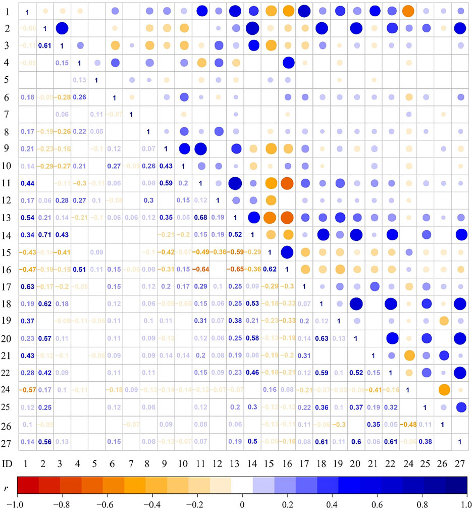
FIGURE 6. Pearson’s correlation coefficient matrix of the continuous covariates used in this research. ID number corresponds to the acronym of covariates in Table 3. The range of Pearson’s correlation coefficients r lies between −1 and 1, and the larger modulus |r| value stands for more significant collinearity. r = 0 indicates no correlation. r > 0 demonstrates that there is a positive correlation that one increases with the increase of other covariates. Conversely, r < 0 means a minus linear dependency.

Receiver Operating Characteristic Curves

Receiver operating characteristic (ROC) curves and their integrated area under curves (AUCs) can be used to assess model performance, including the fitting and prediction skill (Hosmer and Lemeshow, 2000). The ROC is obtained by plotting the true positive rate (TPR, Eq. 3) against the false positive rate (FPR, Eq. 4). The AUC value spans from 0.5 (random guess) to 1 (ideal fit or predictions), and the overall model performance can be recognized as a function of AUC values and classed as follows (Hosmer and Lemeshow, 2000): 1) 0.7 < AUC ≤0.8, acceptable; 2) 0.8 < AUC ≤ 0.9, excellent; and 3) AUC>0.9 outstanding performance.

$TPR=\frac{TP}{TP+FN},(3)$

$FPR=\frac{FP}{TN+FP},(4)$

where false positive (FP)/false negative (FN) represents the number of misclassified landslide/non-landslide samples, and true positive (TP)/true negative (TN) represents the number of landslide/non-landslide classified correctly.

Results

Covariates’ Effects

The regression coefficients of those examined covariates obtained for each model we built with the multi-temporal landslide inventory, that is, pre-seismic Mod1, co-seismic Mod2, and post-seismic Mod3 are shown in Figure 7. A total of 12 variables were significant in at least one of the three models out of all the 26 continuous covariates (see Table 3). Due to each of the continuous variables being rescaled with mean zero and unit variance, the covariate effects reported in Figure 7 are all on the same scale and directly comparable. The regression coefficient values above the zero line indicate a significant positive contribution to landslide occurrence, and symmetry values below the zero line correspond to significant negative effects.

FIGURE 7

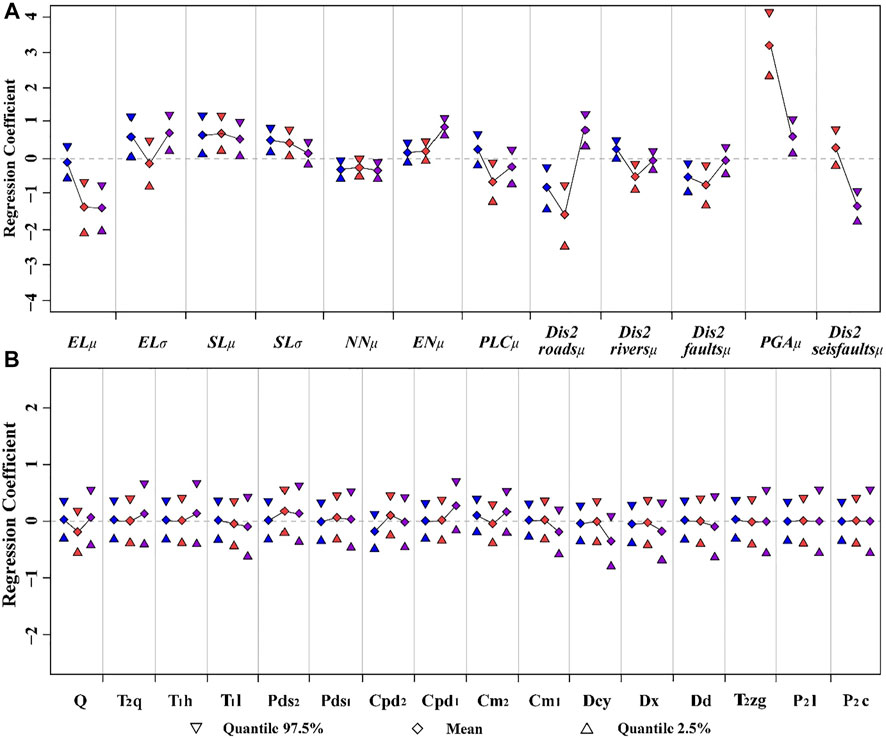
FIGURE 7. Regression coefficients of (A) continuous covariates whose coefficients were significant in at least one of the three models and (B) lithology (Codes correspond to the strata in Tables 1, 3) for each landslide inventory-based susceptibility model Mod1 (blue), Mod2 (red), and Mod3 (purple). A 95% credible interval is expressed as the difference between the quantiles of 97.5 and 2.5. The gray dash line corresponds to zero or no contribution to the model.

As shown in Figure 7, the continuous covariates’ (see Figure 7A) and categorical fixed effects (see Figure 7B) of each model are reported by the mean regression coefficient and the associated 95% credible interval. Overall, some covariates play a dominant role in the model, and the majority of covariates have a limited credible interval. Specifically, for Mod1, the most relevant covariate is the mean slope, which positively contributes to the landslide occurrence (we utilized the mean regression coefficient β to describe the covariates’ effects, hereafter, β_SLµ = 0.665). In contrast, Dis2roadsμ shows a negative contribution (β = −0.809). For the co-seismic Mod2, the mean of PGA appears to dominate the susceptibility pattern with the contribution (positive, β = 3.199) in the absolute value much larger than any other covariate, whereas Dis2roadsµ (β = −1.574) shows a similarly negative contribution to the landslide with Mod1. With the post-seismic Mod3, the mean Dis2seisfault (negative, β = −1.366) and elevation (negative, β = −1.417), in the absolute value, show the greatest degree of negative influence for the slope instability. In all three models, some covariates appear to play the same role, such as the regression coefficient of the mean elevation per SU appears to be negative. The possible reason is that most of the landslides were recognized in the lower portions of the topography in the study area (see Figure 1B). The SLµ positively contributes to the slope instability (β_Mod1 = 0.665, β_Mod2 = 0.713, and β_Mod3 = 0.526); this is consistent with the general knowledge that landslides generally trigger in the steep terrain. The mean of northness appears to have a similar negative effect on the landslide occurrence, which may be due to the decrease in the solar radiation exposure with the increase in northness (β_Mod1 = −0.305, β_Mod2 = −0.246, and β_Mod3 = −0.309). In terms of the mean Dis2faults (β_Mod1 = −0.517, β_Mod2 = −0.736, and β_Mod3 = −0.073), it shows a negative contribution to the landslide occurrence because a greater extent of weathered and fractured rock masses around the faults would decrease the slope stability. Ultimately, RSP, TWI, and PRC showed no significance in all models.

For all three models, lithology does not appear to be significant because the zero line crosses the distribution of each categorical class (Figure 7B). For Mod1, two classes show the slightly significant for the landslides, that is, Cpd₂ chert limestone, bioclastic rock (negatively, β = −0.179) and Cm₂ bioclastic limestone, dolomitic limestone with chert limestone (positively, β = 0.102), while the other classes to the susceptibility are negligible. For Mod2, two classes show the slightly significant for the landslides, Quaternary eluvium, alluvial and diluvial deposits, colluvium and diluvium deposits (negatively, β = −0.193), and Pds₂ limestone intercalated with metamorphic siltstone and slate (positively, β = 0.170). For Mod3, Cpd₁ limestone mixed with clastic limestone (positively, β = 0.277) and Dcy bioclastic limestone and chert-bearing limestone with gravel limestone (negatively, β = −0.349) show the most relevant to the landslides out of these outcropping lithology classes.

Landslide Susceptibility Mapping

Table.4 and Figures 8A–F show the derived landslide susceptibility results (mean probability and the uncertainty). The equal spacing method was used to reclassify the mean susceptibility into five classes: very low (0∼0.2), low (0.2∼0.4), moderate (0.4∼0.6), high (0.6∼0.8), and very high (0.8∼1). According to Table 4, six SUs are highly susceptible to landslide occurrence, whereas 3 years after the Jiuzhaigou earthquake, 57 SUs (accounting for 4.62% of the total SUs) were highly susceptible to instability. The number of slopes with very high susceptibility increased from only one (pre-seismic) to 21 (post-seismic). For the pre- and post-earthquake periods, the very high landslide susceptibility areas are mainly distributed along the valleys, especially the Shuzheng valley and Zechawa valley for the pre-earthquake period, whereas the Rize valley and Panda Lake, which are closer to the epicenter, for the post-earthquake period. In contrast, the co-seismic susceptibility map shows clustered around the epicenter of the earthquake and a southward decreasing trend. Moreover, the pre- and post-seismic uncertainty maps follow a similar pattern to the mean susceptibility maps. In the case of co-seismic landslides, the uncertainty associated with the mean susceptibility appears to be relatively small in the southernmost sector of the study area, although it has a considerably greater spread to the north.

TABLE 4

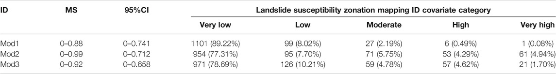
TABLE 4. Mean susceptibility (MS) and its classification (the count of SUs in each class and their percentages), as well as 95% confidence interval, (CI) for each susceptibility model.

FIGURE 8

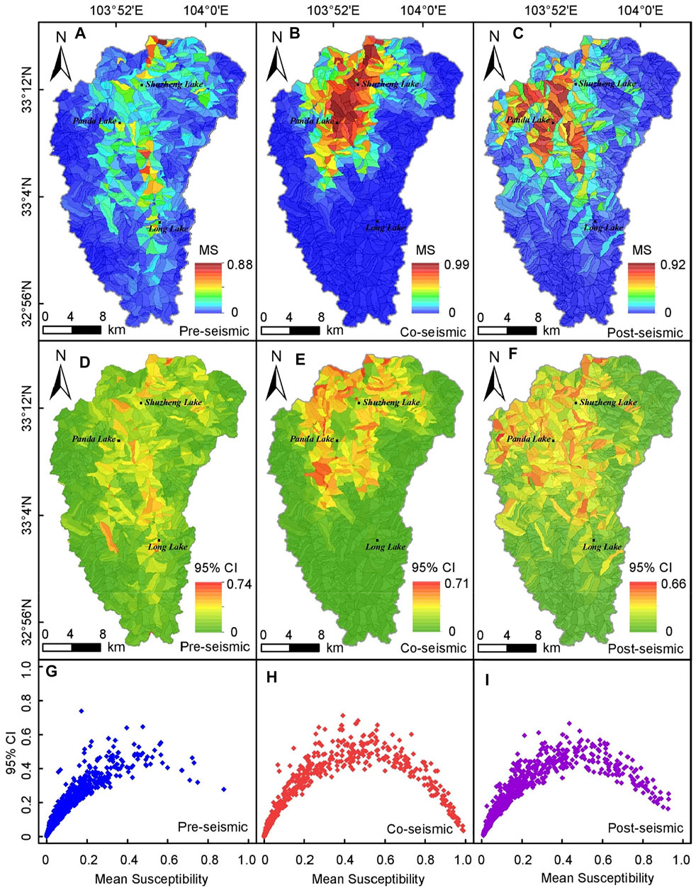
FIGURE 8. (A–C) Mean susceptibility, (D–F) the uncertainty (95% confidence interval) maps, and (G–I) error plot of each multi-temporal landslide inventory-based susceptibility model, corresponding to Mod1 (left), Mod2 (middle), and Mod3 (right panel).

The error plot (Figures 8G–I) shows the mean susceptibility against its associated uncertainty measured in a 95% confidence interval (CI) per SU of each space-time model. It is crucial for determining if the estimates of constructed models are reasonably acceptable in the landslide susceptibility studies (Rossi et al., 2010). The left and right tails of the mean probability distribution should be associated with a very limited uncertainty for an ideal model (Reichenbach et al., 2018). Compared to the pre-seismic (Figure 8G) uncertainty map, the error plots of co-seismic (Figure 8H) and post-seismic (Figure 8I) maps are much better determined, and this is also proved by the model performance shown in Model Performance.

Model Performance

A performance evaluation step is required for each landslide susceptibility assessment model. Figure 9 shows the ROC curves and AUC values of calibration and 10-fold cross-validation results for each model. Although all models produce excellent and outstanding results according to the Hosmer and Lemeshow (2000) classification, Mod2 appears to be outperforming the other two models both in terms of estimated fitting and cross-validation results. More specifically, the fitness results of AUC values for Mod1, Mod2, and Mod3 are 0.838, 0.956, and 0.910 (Figure 9A), respectively, corresponding to be excellent and the rest two for outstanding goodness-of-fit. Also, the validation scheme (see Figures 9B–D for ROCs and associated AUCs distribution) generally performs worse than the corresponding fitting in Figure 9A; the average AUCs 0.801, 0.942, and 0.880 of Mod1, Mod2, and Mod3, respectively, showed the excellent prediction capability for potential slope failure. Our results show that the BLR model has good applicability in predictive performance with outstanding AUC results both for non-seismic, co-seismic, and post-seismic landslide datasets, which is consistent with the grid-based Jiuzhaigou co-seismic landslide susceptibility assessment outcomes in Fan et al. (2018b) (AUC = 0.851) and Ma et al. (2019) (AUC = 0.89). As the validation database changes, a limited variability between the minimum and maximum AUC in the resulting 10 AUCs is observed, that is, 0.069 (AUC_max = 0.976, AUC_min = 0.907) for Mod2 and 0.15 (AUC_max = 0.880, AUC_min = 0.809) for Mod3, although this cannot be said same for the pre-seismic Mod1 which has a significant variability (0.315, AUC_max = 0.926, AUC_min = 0.611). A minor variability of AUCs indicates a more robust predictive model performance that did not change much with the training and test subset replicates in a cross-validation scheme.

FIGURE 9

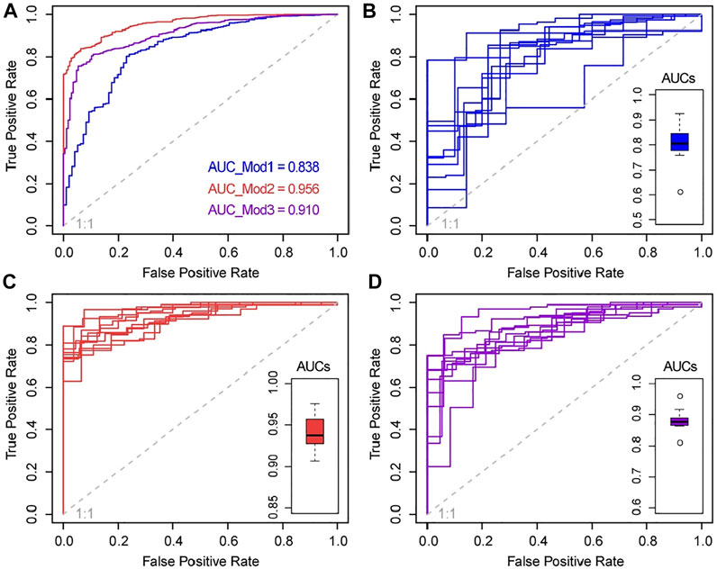
FIGURE 9. Receiver operating characteristic (ROC) curves for (A) the actual calibration and 10-fold cross-validation associated AUC values distribution boxplot for each model corresponding to (B) Mod1, (C) Mod2, and (D) Mod3, respectively. The gray dash line is the reference line (AUC = 0.5), which represents a purely random guess.

Discussion

Strong earthquakes can have a considerable impact on geological conditions, and the seismically induced jointed slopes are vulnerable to becoming potential post-earthquake landslides during subsequent rainfall or earthquakes. The preparation of event-based multi-temporal landslide dataset is an operationally challenging, time-consuming, and potentially expensive process. Lombardo et al. (2020) concluded that the lack of an accurate multi-temporal landslide dataset, rather than the availability of advanced statistical modeling tools, is the fundamental constraint to construct the robust space-time landslide susceptibility models. Due to the absence of the multi-temporal landslide inventory before and after the Jiuzhaigou earthquake, barely anything about the variability of landslide spatial distributions and conditioning factors was known for now. Nevertheless, Guo et al. (2021) tracked the spatio-temporal characteristics of landslides and their changes after the Jiuzhaigou earthquake; the author ignored the pre-seismic, i.e., non-seismic landslides, and the importance variability of landslide conditioning factors. Within 3 years after the 2017 M_w 6.5 Jiuzhaigou earthquake occurred, we utilized a set of satellite imagery to map the pre-, co-, and post-seismic landslides and conducted multi-temporal landslide susceptibility modeling to predict the landslide behavior for the severely affected area—Jiuzhaigou National Geopark (a famous UNESCO world heritage site) in Sichuan, China. In our case study, we attempted to track the variability of spatial distribution of pre-, co-, and post-seismic landslides by using the binary logistic regression (BLR) model for the period between 2017 and 2020.

To explore the importance variability of conditioning factors over time, we calculated the relative importance of covariates according to the value of the regression coefficient in each model (see Figure 7), which are shown in Figure 10. It is observed that the mean Dis2roadways and SLμ had the greatest influence on the occurrence of landslides before the strike of the M_w 6.5 Jiuzhaigou earthquake. It demonstrated the close relationship between human activities (slope cutting) and topography such as elevation and slope angle. Moreover, the importance of the mean Dis2roads and slope, as well as SLσ, decreases with the post-seismic landscape evolution in the study area. In contrast, the importance of the mean of elevation increased from the pre-seismic bottom to the post-seismic top. Besides, the Disfaultsμ shows an increasing importance role in landsliding during the earthquake period, whereas barely any contribution to the landslide occurrence occurred during the post-earthquake period, which is possibly due to the strong effect of seismic shaking (that is, PGA) in the Mod3. For the same purpose, Yang (2019) made a comprehensive study on the characteristics of the influencing factors that changed before and after the 2014 Ludian earthquake (M_w = 6.2, Yunnan Province, China) in the earthquake-affected area. The results showed that the influence of elevation and distance to roads on post-earthquake landslide occurrences increases. However, lithology, slope, distance to faults, distance to streams, and rainfall on post-seismic landslides decrease. Fan et al. (2021) also tracked the temporal landslide conditioning factors evolution associated with the Wenchuan earthquake and concluded that the importance of elevation, slope, aspect, lithology, and rainfall decreased significantly, whereas the topographic position index (TPI) and flow accumulation increased for a given temporal window (2005–2011). In addition, Fan et al. (2021) demonstrated that variables’ prediction capability declines over time, whereas the importance of hydro-topographic parameters increases and becomes predominant within a decade. For three cases, it is consistent that the slope has a strong contribution to the non-seismic landslide occurrence, and with the landscape evolution, the importance decreases. However, the contributions of other landslide conditioning factors through time conflict with our findings, probably due to the different patterns of the geo-environmental variables or the magnitude of the seismic intensity.

FIGURE 10

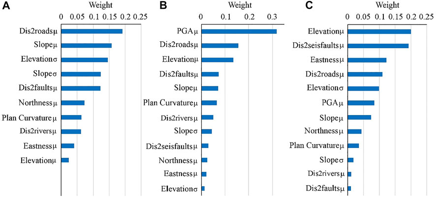
FIGURE 10. Importance order of each significant covariate obtained for each model based on the regression coefficient. (A) Mod1, (B) Mod2, and (C) Mod3.

The factors’ relevance to the model and mean susceptibility can also be observed in the bivariate relationship between mean susceptibility and each covariate shown by smoothed scatter plots for Mod1, Mod2, and Mod3 (see Figure 11). If a covariate played a significant role in the model, its impact on ultimate susceptibility should appear or be noticeable even when the other additive components are taken into account. For instance, when the mean elevation increases from the range of 2002–4865 m, the mean susceptibility in each slope unit decreases on the whole in all three models, although the maximum susceptibility corresponds to different elevation values (2500 m for pre- and co-seismic model and 3000 m for the post-seismic model) (see Figures 11a, A and A′). A positive contribution of the mean of slope to the landslide susceptibility can be easily interpreted for all models because the mean susceptibility increases immediately with the increase in the mean of slope. Also, compared with the co-seismic and post-seismic dataset, the high value of mean susceptibility of the pre-seismic dataset was distributed in a much more concentrated slope range (30°–40°) for the pre-seismic dataset (Figures 11b, B and B′). It means the mean of slope plays a dominant role in Mod1, and the relative importance decreases with the drift of time in the study area. As shown in Figures 11c, C and C′, the negative relationship between the Dis2roadsμ and mean susceptibility during the whole period means the closer to the roadways, the higher the possibility landslide occurs, especially for the range of 0–2000m in Mod1 and Mod2, but a much larger range of 0–8000 m in Mod3. For Dis2faultsμ (Figures 11d, D and D′), the susceptibility shows a similar decreasing trend with the increase in the distance as the Dis2roadsμ. For the seismic factors (PGA (Figures 11e, E and E′) and the distance to the causative fault (Figures 11f, F and F′)), the roles in Mod2 and Mod3 are almost the same, showing the long-term effect of ground motion and the closer to the epicenter and seismogenic fault, the larger impact on the geo-environment.

FIGURE 11

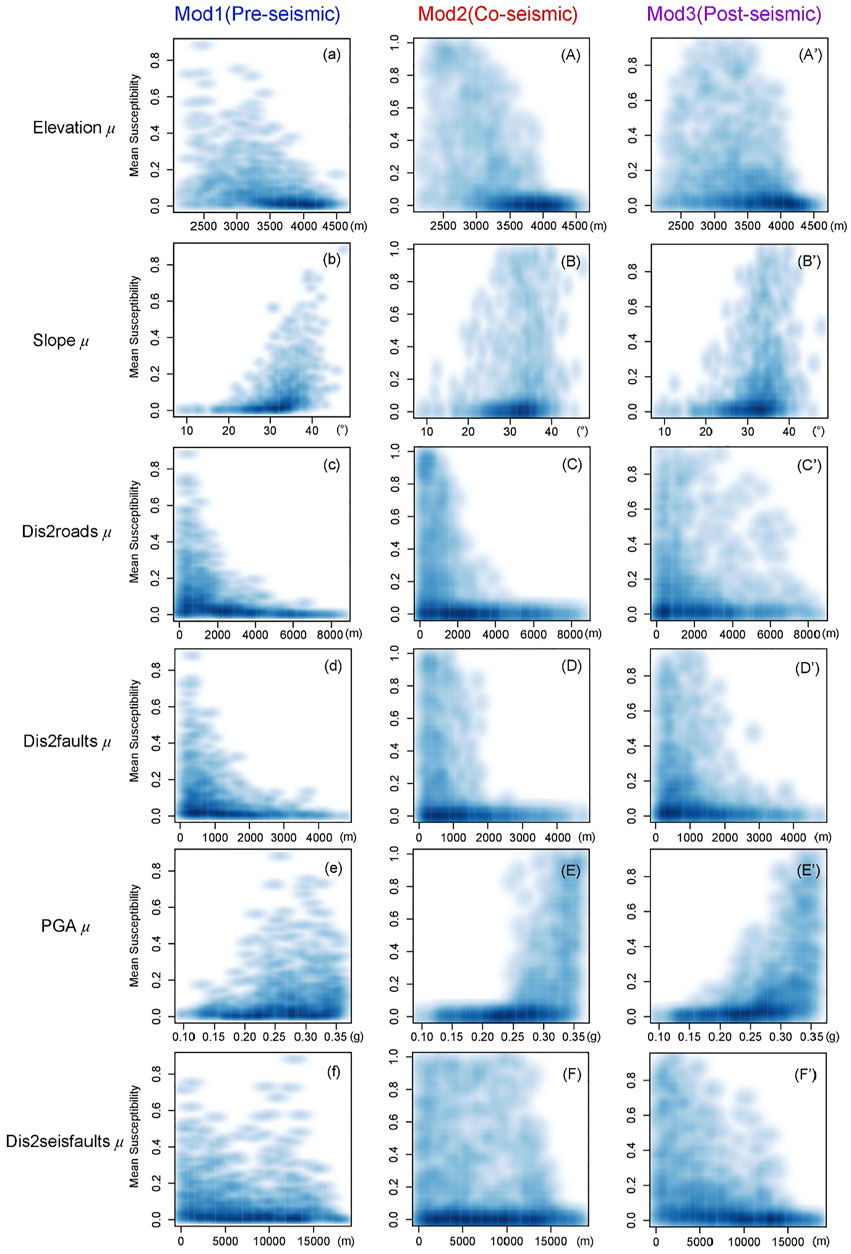
FIGURE 11. Two-dimensional (kernel density) smoothed scatter plots showing the bivariate relationship between the mean susceptibility and each covariate for Mod1 (left panel), Mod2 (middle panel), and Mod3 (right panel).

Ultimately, our findings show that there are variations in both landslide conditioning factors and susceptibility maps through time. This result is also supported by Kincey et al. (2021), who found significant changes in the characteristics and distributions of co-seismic and monsoon-triggered landslides in Nepal from 2014 to 2018. Thus, as many as multi-temporal landslide inventories are required to estimate the time-dependent effect on the landslide susceptibility over a longer period or in response to several events. Otherwise, it will be negatively biased (Samia et al., 2017). Notably, our knowledge of the possible effects of the time-dependent landslide occurrence on landslide susceptibility remains inadequate, posing a substantial source of uncertainty with important implications for landslide susceptibility modeling. The results can be the reference for the prediction of the probability of potential landslides and geological environmental protection in the world heritage Jiuzhaigou mountainous area.

Conclusion

Landslide susceptibility modeling over time scales for a single trigger (e.g., earthquake and rainstorm) was relatively uncommon in prior studies. In this study, we conducted a case study of multi-temporal statistical landslide susceptibility modeling across the pre-, co-, and post-seismic phases. Three landslide inventory datasets, including 154 pre-seismic, 1022 co-seismic, and 364 post-seismic landslides, respectively, and spatio-temporal variations of landslide spatial susceptibility and covariates’ effects were obtained. The slope unit-based binary logistic regression (BLR) model shows a good predictive applicability with outstanding performance for the Jiuzhaigou area. Moreover, our results show that there are variations in both landslide conditioning factors and susceptibility maps through time. Furthermore, human activity and slope contribute most to the pre-seismic landslide occurrence. Meanwhile, PGA dominates the co-seismic landslide susceptibility pattern, and the distance to the seismogenic fault and elevation show the most significant degree of influence to the post-seismic slope instability. The number of SUs with a mean probability over 0.8 from only one (pre-seismic) increased to 21 (post-seismic). The spatial and temporal dynamical changes of landslides highlight the necessity to carry out continuous landslide monitoring and analyses over a longer period or in response to extreme events at a regional scale. It is worth mentioning that the findings could be different in the other geo-environmental setting and seismic magnitude conditions. Therefore, our conclusions still need to be verified through more earthquake-induced landslide inventories and areas in other contexts. Also, further understanding of the post-seismic landslide changes for the Jiuzhaigou area could also be made by a much more frequent or prolonged observational time.

Data Availability Statement

The original contributions presented in the study are included in the article/Supplementary Material, further inquiries can be directed to the corresponding author.

Author Contributions

LL and XP conceived and designed the experiments; LL and CZ performed the experiments; LL and QY analyzed the data; LL and XP wrote the manuscript; XF, LZ, and RH revised the manuscript.

Funding

This study was financially supported by the National Natural Science Foundation of China (Grant No. 41931296), the National Key R&D Program of China (No. 2017YFC1501002), and the National Nature Science Foundation of China (Grant Nos. 41907254 and 41521002).

Conflict of Interest

Author CZ was employed by the Chengdu Surveying Geotechnical Research Institute Co., Ltd.

The remaining authors declare that the research was conducted in the absence of any commercial or financial relationships that could be construed as a potential conflict of interest.

Publisher’s Note

All claims expressed in this article are solely those of the authors and do not necessarily represent those of their affiliated organizations, or those of the publisher, the editors, and the reviewers. Any product that may be evaluated in this article, or claim that may be made by its manufacturer, is not guaranteed or endorsed by the publisher.

Acknowledgments

The authors would like to thank Prof. Cees van Westen for his constructive comments to improve the quality of our manuscript.

References

Allen, T. I., Wald, D. J., Hotovec, A. J., Lin, K., Earle, P. S., and Marano, K. D. (2008). An Atlas of ShakeMaps for Selected Global Earthquakes. Reston, VA: US Department of the Interior, US Geological Survey, 35.

Google Scholar

Alvioli, M., Marchesini, I., Reichenbach, P., Rossi, M., Ardizzone, F., Fiorucci, F., et al. (2016). Automatic Delineation of Geomorphological Slope Units with r.Slopeunits v1.0 and Their Optimization for Landslide Susceptibility Modeling. Geosci. Model. Dev. 9 (11), 3975–3991. doi:10.5194/gmd-9-3975-2016

CrossRef Full Text | Google Scholar

Amato, G., Eisank, C., Castro-Camilo, D., and Lombardo, L. (2019). Accounting for Covariate Distributions in Slope-Unit-Based Landslide Susceptibility Models. A Case Study in the alpine Environment. Eng. Geology. 260, 105237. doi:10.1016/j.enggeo.2019.105237

CrossRef Full Text | Google Scholar

Beven, K. J., and Kirkby, M. J. (1979). A physically based, variable contributing area model of basin hydrology/Un modèle à base physique de zone d'appel variable de l'hydrologie du bassin versant. Hydrological Sci. Bull. 24 (1), 43–69. doi:10.1080/02626667909491834

CrossRef Full Text | Google Scholar

Brabb, E. E. (1985). “Innovative Approaches to Landslide hazard and Risk Mapping,” in International Landslide Symposium Proceedings, Toronto, Canada, Japan, August 23-31, 1985 1, 17–22.

Google Scholar

Brenning, A. (2005). Spatial Prediction Models for Landslide Hazards: Review, Comparison and Evaluation. Nat. Hazards Earth Syst. Sci. 5 (6), 853–862. doi:10.5194/nhess-5-853-2005

CrossRef Full Text | Google Scholar

Böhner, J., and Selige, T. (2006). “Spatial Prediction of Soil Attributes Using Terrain Analysis and Climate Regionalisation,” in Analysis and Modelling Applications (Göttinger: Göttinger Geographische Abhandlungen), 13–28.

Google Scholar

Cao, J., Zhang, Z., Du, J., Zhang, L., Song, Y., and Sun, G. (2020). Multi-geohazards Susceptibility Mapping Based on Machine Learning-A Case Study in Jiuzhaigou, China. Nat. Hazards 102 (3), 851–871. doi:10.1007/s11069-020-03927-8

CrossRef Full Text | Google Scholar

Carrara, A., Cardinali, M., Guzzetti, F., and Reichenbach, P. (1995). “GIS Technology in Mapping Landslide hazard,” in Geographical Information Systems in Assessing Natural Hazards (New York: Springer), 135–175. doi:10.1007/978-94-015-8404-3_8

CrossRef Full Text | Google Scholar

Chen, W., Pourghasemi, H. R., Panahi, M., Kornejady, A., Wang, J., Xie, X., et al. (2017). Spatial Prediction of Landslide Susceptibility Using an Adaptive Neuro-Fuzzy Inference System Combined with Frequency Ratio, Generalized Additive Model, and Support Vector Machine Techniques. Geomorphology 297, 69–85. doi:10.1016/j.geomorph.2017.09.007

CrossRef Full Text | Google Scholar

Chen, X.-l., Shan, X.-j., Wang, M.-m., Liu, C.-g., and Han, N.-n. (2020). Distribution Pattern of Coseismic Landslides Triggered by the 2017 Jiuzhaigou Ms 7.0 Earthquake of China: Control of Seismic Landslide Susceptibility. Ijgi 9 (4), 198. doi:10.3390/ijgi9040198

CrossRef Full Text | Google Scholar

Cui, P., Liu, S., Tang, B., and Chen, X. (2005). Research and Prevention of Debris Flow in National parks. Beijing, China: Science Press.

Google Scholar

Cui, S., Pei, X., Jiang, Y., Wang, G., Fan, X., Yang, Q., et al. (2021). Liquefaction within a Bedding Fault: Understanding the Initiation and Movement of the Daguangbao Landslide Triggered by the 2008 Wenchuan Earthquake (Ms = 8.0). Eng. Geology. 295, 106455. doi:10.1016/j.enggeo.2021.106455

CrossRef Full Text | Google Scholar

Fan, X., Domènech, G., Scaringi, G., Huang, R., Xu, Q., Hales, T. C., et al. (2018a). Spatio-temporal Evolution of Mass Wasting after the 2008 Mw 7.9 Wenchuan Earthquake Revealed by a Detailed Multi-Temporal Inventory. Landslides 15 (12), 2325–2341. doi:10.1007/s10346-018-1054-5

CrossRef Full Text | Google Scholar

Fan, X., Scaringi, G., Domènech, G., Yang, F., Guo, X., Dai, L., et al. (2019a). Two Multi-Temporal Datasets that Track the Enhanced Landsliding after the 2008 Wenchuan Earthquake. Earth Syst. Sci. Data 11 (1), 35–55. doi:10.5194/essd-11-35-2019

CrossRef Full Text | Google Scholar

Fan, X., Scaringi, G., Korup, O., West, A. J., Westen, C. J., Tanyas, H., et al. (2019b). Earthquake‐Induced Chains of Geologic Hazards: Patterns, Mechanisms, and Impacts. Rev. Geophys. 57 (2), 421–503. doi:10.1029/2018rg000626

CrossRef Full Text | Google Scholar

Fan, X., Scaringi, G., Xu, Q., Zhan, W., Dai, L., Li, Y., et al. (2018b). Coseismic Landslides Triggered by the 8th August 2017 Ms 7.0 Jiuzhaigou Earthquake (Sichuan, China): Factors Controlling Their Spatial Distribution and Implications for the Seismogenic Blind Fault Identification. Landslides 15 (5), 967–983. doi:10.1007/s10346-018-0960-x

CrossRef Full Text | Google Scholar

Fan, X., Yunus, A. P., Scaringi, G., Catani, F., Siva Subramanian, S., Xu, Q., et al. (2021). Rapidly Evolving Controls of Landslides after a strong Earthquake and Implications for hazard Assessments. Geophys. Res. Lett. 48 (1), e2020GL090509. doi:10.1029/2020gl090509

CrossRef Full Text | Google Scholar

Fell, R., Corominas, J., Bonnard, C., Cascini, L., Leroi, E., and Savage, W. Z. (2008). Guidelines for Landslide Susceptibility, hazard and Risk Zoning for Land-Use Planning. Eng. Geology. 102 (3-4), 99–111. doi:10.1016/j.enggeo.2008.03.014

CrossRef Full Text | Google Scholar

Furlani, S., and Ninfo, A. (2015). Is the Present the Key to the Future? Earth-Science Rev. 142, 38–46. doi:10.1016/j.earscirev.2014.12.005

CrossRef Full Text | Google Scholar

Galli, M., Ardizzone, F., Cardinali, M., Guzzetti, F., and Reichenbach, P. (2008). Comparing Landslide Inventory Maps. Geomorphology 94 (3-4), 268–289. doi:10.1016/j.geomorph.2006.09.023

CrossRef Full Text | Google Scholar

Guo, X., Fu, B., Du, J., Shi, P., Li, J., Li, Z., et al. (2021). Monitoring and Assessment for the Susceptibility of Landslide Changes after the 2017 Ms 7.0 Jiuzhaigou Earthquake Using the Remote Sensing Technology. Front. Earth Sci. 9, 633117. doi:10.3389/feart.2021.633117

CrossRef Full Text | Google Scholar

Guzzetti, F., Carrara, A., Cardinali, M., and Reichenbach, P. (1999). Landslide hazard Evaluation: A Review of Current Techniques and Their Application in a Multi-Scale Study, central Italy. Geomorphology 31 (1), 181–216. doi:10.1016/s0169-555x(99)00078-1

CrossRef Full Text | Google Scholar

Guzzetti, F., Galli, M., Reichenbach, P., Ardizzone, F., and Cardinali, M. (2006). Landslide hazard Assessment in the Collazzone Area, Umbria, Central Italy. Nat. Hazards Earth Syst. Sci. 6 (1), 115–131. doi:10.5194/nhess-6-115-2006

CrossRef Full Text | Google Scholar

Harp, E. L., Keefer, D. K., Sato, H. P., and Yagi, H. (2011). Landslide Inventories: the Essential Part of Seismic Landslide hazard Analyses. Eng. Geology. 122 (1-2), 9–21. doi:10.1016/j.enggeo.2010.06.013

CrossRef Full Text | Google Scholar

He, Y., and Kusiak, A. (2017). Performance Assessment of Wind Turbines: Data-Derived Quantitative Metrics. IEEE Trans. Sustain. Energ. 9 (1), 65–73.

Google Scholar

Heerdegen, R. G., and Beran, M. A. (1982). Quantifying Source Areas through Land Surface Curvature and Shape. J. Hydrol. 57 (3-4), 359–373. doi:10.1016/0022-1694(82)90155-x

CrossRef Full Text | Google Scholar

Hosmer, D. W., and Lemeshow, S. (2000). Applied Logistic Regression. Second edition. New York: Wiley.

Google Scholar

Hu, X., Hu, K., Tang, J., You, Y., and Wu, C. (2019). Assessment of Debris-Flow Potential Dangers in the Jiuzhaigou valley Following the August 8, 2017, Jiuzhaigou Earthquake, Western China. Eng. Geology. 256, 57–66. doi:10.1016/j.enggeo.2019.05.004

CrossRef Full Text | Google Scholar

Huang, R., and Li, W. (2014). Post-earthquake Landsliding and Long-Term Impacts in the Wenchuan Earthquake Area, china. Eng. Geology. 182, 111–120. doi:10.1016/j.enggeo.2014.07.008

CrossRef Full Text | Google Scholar

Hungr, O., Leroueil, S., and Picarelli, L. (2014). The Varnes Classification of Landslide Types, an Update. Landslides 11 (2), 167–194. doi:10.1007/s10346-013-0436-y

CrossRef Full Text | Google Scholar

Hussin, H. Y., Zumpano, V., Reichenbach, P., Sterlacchini, S., Micu, M., van Westen, C., et al. (2016). Different Landslide Sampling Strategies in a Grid-Based Bi-variate Statistical Susceptibility Model. Geomorphology 253, 508–523. doi:10.1016/j.geomorph.2015.10.030

CrossRef Full Text | Google Scholar

Kamp, U., Growley, B. J., Khattak, G. A., and Owen, L. A. (2008). GIS-based Landslide Susceptibility Mapping for the 2005 Kashmir Earthquake Region. Geomorphology 101 (4), 631–642. doi:10.1016/j.geomorph.2008.03.003

CrossRef Full Text | Google Scholar

Keefer, D. K. (2002). Investigating Landslides Caused by Earthquakes-A Historical Review. Surv. Geophys. 23 (6), 473–510. doi:10.1023/a:1021274710840

CrossRef Full Text | Google Scholar

Keefer, D. K. (1984). Landslides Caused by Earthquakes. Geol. Soc. America Bull. 95 (4), 406–421. doi:10.1130/0016-7606(1984)95<406:lcbe>2.0.co;2

CrossRef Full Text | Google Scholar

Kelava, A., Moosbrugger, H., Dimitruk, P., and Schermelleh-Engel, K. (2008). Multicollinearity and Missing Constraints. Methodology 4 (2), 51–66. doi:10.1027/1614-2241.4.2.51

CrossRef Full Text | Google Scholar

Khattak, G. A., Owen, L. A., Kamp, U., and Harp, E. L. (2010). Evolution of Earthquake-Triggered Landslides in the Kashmir Himalaya, Northern Pakistan. Geomorphology 115 (1-2), 102–108. doi:10.1016/j.geomorph.2009.09.035

CrossRef Full Text | Google Scholar

Kincey, M. E., Rosser, N. J., Robinson, T. R., Densmore, A. L., Shrestha, R., Pujara, D. S., et al. (2021). Evolution of Coseismic and post-seismic Landsliding after the 2015 M_w 7.8 Gorkha Earthquake, Nepal. J. Geophys. Res. Earth Surf. 126, e2020JF005803. doi:10.1029/2020jf005803

CrossRef Full Text | Google Scholar

Lee, C. T., Huang, C. C., Lee, J. F., Pan, K. L., Lin, M. L., and Dong, J. J. (2008). Statistical Approach to Earthquake-Induced Landslide Susceptibility. Eng. Geology. 100 (1-2), 43–58. doi:10.1016/j.enggeo.2008.03.004

CrossRef Full Text | Google Scholar

Li, C., Xu, W., Wu, J., and Gao, M. (2016). Using New Models to Assess Probabilistic Seismic hazard of the North-South Seismic Zone in China. Nat. Hazards 82 (1), 659–681. doi:10.1007/s11069-016-2212-5

CrossRef Full Text | Google Scholar

Li, H., Deng, J., Feng, P., Pu, C., Arachchige, D. D., and Cheng, Q. (2021b). Short-Term Nacelle Orientation Forecasting Using Bilinear Transformation and ICEEMDAN Framework. Front. Energ. Res. 697. doi:10.3389/fenrg.2021.780928

CrossRef Full Text | Google Scholar

Li, H., Deng, J., Yuan, S., Feng, P., and Arachchige, D. D. (2021a). Monitoring and Identifying Wind Turbine Generator Bearing Faults Using Deep Belief Network and EWMA Control Charts. Front. Energ. Res. 9. doi:10.3389/fenrg.2021.799039

CrossRef Full Text | Google Scholar

Li, H., He, Y., Xu, Q., Deng, J., Li, W., and Wei, Y. (2022). Detection and Segmentation of Loess Landslides via Satellite Images: a Two-phase Framework. Landslides 19 (3), 673–686. doi:10.1007/s10346-021-01789-0

CrossRef Full Text | Google Scholar

Lin, C. W., Liu, S. H., Lee, S. Y., and Liu, C. C. (2006). Impacts of the Chi-Chi Earthquake on Subsequent Rainfall-Induced Landslides in central Taiwan. Eng. Geology. 86 (2-3), 87–101. doi:10.1016/j.enggeo.2006.02.010

CrossRef Full Text | Google Scholar

Ling, S., Sun, C., Li, X., Ren, Y., Xu, J., and Huang, T. (2021). Characterizing the Distribution Pattern and Geologic and Geomorphic Controls on Earthquake-Triggered Landslide Occurrence during the 2017 Ms 7.0 Jiuzhaigou Earthquake, Sichuan, China. Landslides 18 (4), 1275–1291. doi:10.1007/s10346-020-01549-6

CrossRef Full Text | Google Scholar

Lombardo, L., Opitz, T., Ardizzone, F., Guzzetti, F., and Huser, R. (2020). Space-time Landslide Predictive Modelling. Earth-Science Rev. 209, 103318. doi:10.1016/j.earscirev.2020.103318

CrossRef Full Text | Google Scholar

Lombardo, L., Saia, S., Schillaci, C., Mai, P. M., and Huser, R. (2018). Modeling Soil Organic Carbon with Quantile Regression: Dissecting Predictors' Effects on Carbon Stocks. Geoderma 318, 148–159. doi:10.1016/j.geoderma.2017.12.011

CrossRef Full Text | Google Scholar

Luo, L., Lombardo, L., van Westen, C., Pei, X., and Huang, R. (2021). “From Scenario-Based Seismic hazard to Scenario-Based Landslide hazard: Rewinding to the Past via Statistical Simulations,” in Stochastic Environmental Research and Risk Assessment, 1–22. doi:10.1007/s00477-020-01959-x

CrossRef Full Text | Google Scholar

Ma, S., Xu, C., Tian, Y., and Xu, X. (2019). Application of Logistic Regression Model for hazard Assessment of Earthquake-Triggered Landslides: A Case Study of 2017 Jiuzhaigou (China) Ms 7.0 Event. Seismology Geology. 41 (1), 162–177. (in Chinese). doi:10.3969/j.issn.0253-4967.2019.01.011

CrossRef Full Text | Google Scholar

Marc, O., Hovius, N., Meunier, P., Uchida, T., and Hayashi, S. (2015). Transient Changes of Landslide Rates after Earthquakes. Geology 43 (10), 883–886. doi:10.1130/g36961.1

CrossRef Full Text | Google Scholar

Micheletti, N., Foresti, L., Robert, S., Leuenberger, M., Pedrazzini, A., Jaboyedoff, M., et al. (2014). Machine Learning Feature Selection Methods for Landslide Susceptibility Mapping. Math. Geosci. 46 (1), 33–57. doi:10.1007/s11004-013-9511-0

CrossRef Full Text | Google Scholar

Montgomery, D. R., and Dietrich, W. E. (1994). A Physically Based Model for the Topographic Control on Shallow Landsliding. Water Resour. Res. 30 (4), 1153–1171. doi:10.1029/93wr02979

CrossRef Full Text | Google Scholar

Moore, D. S., Notz, W. I., and Notz, W. (2006). Statistics: Concepts and Controversies. New York: Macmillan.

Google Scholar

Newmark, N. M. (1965). Effects of Earthquakes on Dams and Embankments. Géotechnique 15 (2), 139–160. doi:10.1680/geot.1965.15.2.139

CrossRef Full Text | Google Scholar

Nowicki Jessee, M. A., Hamburger, M. W., Allstadt, K., Wald, D. J., Robeson, S. M., Tanyas, H., et al. (2018). A Global Empirical Model for Near‐Real‐Time Assessment of Seismically Induced Landslides. J. Geophys. Res. Earth Surf. 123 (8), 1835–1859. doi:10.1029/2017jf004494

CrossRef Full Text | Google Scholar

Nowicki, M. A., Wald, D. J., Hamburger, M. W., Hearne, M., and Thompson, E. M. (2014). Development of a Globally Applicable Model for Near Real-Time Prediction of Seismically Induced Landslides. Eng. Geology. 173, 54–65. doi:10.1016/j.enggeo.2014.02.002

CrossRef Full Text | Google Scholar

Reichenbach, P., Rossi, M., Malamud, B. D., Mihir, M., and Guzzetti, F. (2018). A Review of Statistically-Based Landslide Susceptibility Models. Earth-Science Rev. 180, 60–91. doi:10.1016/j.earscirev.2018.03.001

CrossRef Full Text | Google Scholar

Rossi, M., Guzzetti, F., Reichenbach, P., Mondini, A. C., and Peruccacci, S. (2010). Optimal Landslide Susceptibility Zonation Based on Multiple Forecasts. Geomorphology 114 (3), 129–142. doi:10.1016/j.geomorph.2009.06.020

CrossRef Full Text | Google Scholar

Samia, J., Temme, A., Bregt, A., Wallinga, J., Guzzetti, F., Ardizzone, F., et al. (2017). Do landslides Follow Landslides? Insights in Path Dependency from a Multi-Temporal Landslide Inventory. Landslides 14 (2), 547–558. doi:10.1007/s10346-016-0739-x

CrossRef Full Text | Google Scholar

Segoni, S., Tofani, V., Rosi, A., Catani, F., and Casagli, N. (2018). Combination of Rainfall Thresholds and Susceptibility Maps for Dynamic Landslide hazard Assessment at Regional Scale. Front. Earth Sci. 6, 85. doi:10.3389/feart.2018.00085

CrossRef Full Text | Google Scholar

Shrestha, S., and Kang, T.-S. (2019). Assessment of Seismically-Induced Landslide Susceptibility after the 2015 Gorkha Earthquake, Nepal. Bull. Eng. Geol. Environ. 78 (3), 1829–1842. doi:10.1007/s10064-017-1191-4

CrossRef Full Text | Google Scholar

Steger, S., Brenning, A., Bell, R., and Glade, T. (2016). The Propagation of Inventory-Based Positional Errors into Statistical Landslide Susceptibility Models. Nat. Hazards Earth Syst. Sci. 16 (12), 2729–2745. doi:10.5194/nhess-16-2729-2016

CrossRef Full Text | Google Scholar

Strauch, R., Istanbulluoglu, E., and Riedel, J. (2019). A New Approach to Mapping Landslide Hazards: a Probabilistic Integration of Empirical and Physically Based Models in the North Cascades of Washington, USA. Nat. Hazards Earth Syst. Sci. 19 (11), 2477–2495. doi:10.5194/nhess-19-2477-2019

CrossRef Full Text | Google Scholar

Tang, C., Van Westen, C. J., Tanyas, H., and Jetten, V. G. (2016). Analysing post-earthquake Landslide Activity Using Multi-Temporal Landslide Inventories Near the Epicentral Area of the 2008 Wenchuan Earthquake. Nat. Hazards Earth Syst. Sci. 16 (12), 2641–2655. doi:10.5194/nhess-16-2641-2016

CrossRef Full Text | Google Scholar

Tanyas, H., Kirschbaum, D., Gorum, T., van Westen, C. J., and Lombardo, L. (2021a). New Insight into post-seismic Landslide Evolution Processes in the Tropics. Fron. in Earth Sci.

Google Scholar

Tanyaş, H., Kirschbaum, D., and Lombardo, L. (2021b). Capturing the Footprints of Ground Motion in the Spatial Distribution of Rainfall-Induced Landslides. Bull. Eng. Geology. Environ. 80 (6), 4323–4345. doi:10.1007/s10064-021-02238-x

CrossRef Full Text | Google Scholar

Tanyas, H., and Lombardo, L. (2020). Completeness Index for Earthquake-Induced Landslide Inventories. Eng. Geology. 264, 105331. doi:10.1016/j.enggeo.2019.105331

CrossRef Full Text | Google Scholar

Tian, Y., Xu, C., Chen, J., Zhou, Q., and Shen, L. (2017). Geometrical Characteristics of Earthquake-Induced Landslides and Correlations with Control Factors: a Case Study of the 2013 minxian, Gansu, China, Mw 5.9 Event. Landslides 14 (6), 1915–1927. doi:10.1007/s10346-017-0835-6

CrossRef Full Text | Google Scholar

Tian, Y., Xu, C., Ma, S., Xu, X., Wang, S., and Zhang, H. (2019). Inventory and Spatial Distribution of Landslides Triggered by the 8th August 2017 MW 6.5 Jiuzhaigou Earthquake, China. J. Earth Sci. 30 (1), 206–217. doi:10.1007/s12583-018-0869-2

CrossRef Full Text | Google Scholar

Van Westen, C. J., Rengers, N., and Soeters, R. (2003). Use of Geomorphological Information in Indirect Landslide Susceptibility Assessment. Nat. hazards 30 (3), 399–419. doi:10.1023/b:nhaz.0000007097.42735.9e

CrossRef Full Text | Google Scholar

Varnes, D. J. (1984). Landslide hazard Zonation: A Review of Principles and Practice (No. 3).

Google Scholar

Wang, J., Jin, W., Cui, Y.-f., Zhang, W.-f., Wu, C.-h., and Alessandro, P. (2018). Earthquake-triggered Landslides Affecting a UNESCO Natural Site: the 2017 Jiuzhaigou Earthquake in the World National Park, China. J. Mt. Sci. 15 (7), 1412–1428. doi:10.1007/s11629-018-4823-7

CrossRef Full Text | Google Scholar

Wu, C.-h., Cui, P., Li, Y.-s., Ayala, I. A., Huang, C., and Yi, S.-j. (2018). Seismogenic Fault and Topography Control on the Spatial Patterns of Landslides Triggered by the 2017 Jiuzhaigou Earthquake. J. Mt. Sci. 15 (4), 793–807. doi:10.1007/s11629-017-4761-9

CrossRef Full Text | Google Scholar

Xu, C., Dai, F., Xu, X., and Lee, Y. H. (2012). GIS-based Support Vector Machine Modeling of Earthquake-Triggered Landslide Susceptibility in the Jianjiang River Watershed, China. Geomorphology 145-146, 70–80. doi:10.1016/j.geomorph.2011.12.040

CrossRef Full Text | Google Scholar

Yang, D. (2019). Comprehensive Study on Landslide Susceptibility Evaluation and Seismic Effect before and after Earthquake in Qiaojia County. Yunnan province: Kunming University of Technology. (in Chinese).

Google Scholar

Yang, W., Qi, W., Wang, M., Zhang, J., and Zhang, Y. (2017). Spatial and Temporal Analyses of post-seismic Landslide Changes Near the Epicentre of the Wenchuan Earthquake. Geomorphology 276, 8–15. doi:10.1016/j.geomorph.2016.10.010

CrossRef Full Text | Google Scholar

Yi, S.-j., Wu, C.-h., Li, Y.-s., and Huang, C. (2018). Source Tectonic Dynamics Features of Jiuzhaigou Ms 7.0 Earthquake in Sichuan Province, China. J. Mt. Sci. 15 (10), 2266–2275. doi:10.1007/s11629-017-4703-6

CrossRef Full Text | Google Scholar

Yi, Y., Zhang, Z., Zhang, W., Xu, Q., Deng, C., and Li, Q. (2019). GIS-based Earthquake-Triggered-Landslide Susceptibility Mapping with an Integrated Weighted index Model in Jiuzhaigou Region of Sichuan Province, China. Nat. Hazards Earth Syst. Sci. 19 (9), 1973–1988. doi:10.5194/nhess-19-1973-2019

CrossRef Full Text | Google Scholar

Zevenbergen, L. W., and Thorne, C. R. (1987). Quantitative Analysis of Land Surface Topography. Earth Surf. Process. Landforms 12 (1), 47–56. doi:10.1002/esp.3290120107

CrossRef Full Text | Google Scholar

Zhou, J., Wei, J., Yang, T., Zhang, P., Liu, F., and Chen, J. (2021). Seepage Channel Development in the crown Pillar: Insights from Induced Microseismicity. Int. J. Rock Mech. Mining Sci. 145, 104851. doi:10.1016/j.ijrmms.2021.104851

CrossRef Full Text | Google Scholar