Stratified Saline Flume Experiments on the Entrainment Process of the Atmospheric Convective Boundary Layer With Vertical Wind Shear

A stratified saline flume experimental apparatus was set up in this study to experimentally simulate the entrainment process of the atmospheric convective boundary layer with vertical wind shear, of which the entrainment characteristics are quite different from those of the shear-free convective boundary layer. Entrainment occurs at the interface of the flume inlet until the velocity difference between the upper and lower layers reaches 0.04 m/s, and a thin stable entrainment zone is formed at a 12z_i distance from the flow inlet, where z_i is the height of the entrainment zone. Shear in the entrainment zone induces the counter-gradient momentum transport process, and a series of large-scale vortices with a characteristic length of about (1.0–1.5)z_i fills this region. The data analysis shows that the velocity difference and buoyancy flux of the bottom plume promote the occurrence of entrainment, while the density difference between the upper and lower layers inhibits it. The contribution of the shear effect to the entrainment process was introduced into the characteristic velocity scale, and a new scaling relation between the dimensionless thickness of the entrainment zone and the corrected Richardson number was obtained as Δz/z_i = 1.17Ri_NC^−1/2 from the experimental results, which agrees well with the available radar data and the numerical simulation data.

1 Introduction

The atmospheric convective boundary layer (CBL), located within 2000 m above the earth’s surface, is characterized by a significant stratified temperature structure in the depth direction. Especially, when there are different horizontal wind velocities in the upper and lower layers, the flow characteristics of sheared atmospheric CBL are obviously different from those of the shear-free atmospheric CBL. A typical sheared atmospheric CBL, as schematically depicted in Figure 1, consists of four zones: the surface sublayer close to the earth’s surface (about 100 m), the mixed zone (about 1,000 m), the entrainment zone (about 200 m), and the free atmosphere (about 700 m) (Allaerts, 2016). In the mixed zone, the combined strong shear near the surface sublayer and the convection due to the thermal buoyancy from the surface make the atmosphere within it profoundly mixed, resulting in almost constant horizontal velocity and potential temperature gradient, and linearly reduced buoyancy flux. Above the mixed zone, the horizontal velocity gradually increases with height, which creates shear, while the potential temperature gradient also increases gradually; but the buoyancy changes its decreasing trend to be increased at the height z_i, which is defined as the height of the entrainment zone. Beyond the entrainment zone is the free atmosphere where the horizontal velocity becomes constant, the potential temperature increases approximately linearly, and the buoyancy flux is negligible. It is apparent that the material and energy exchanges between the CBL and the free atmosphere above are strongly affected by the characteristics of the entrainment process in the sheared CBL, so its understanding is very important and crucial for the accurate meteorological predictions of the atmospheric CBL.

FIGURE 1

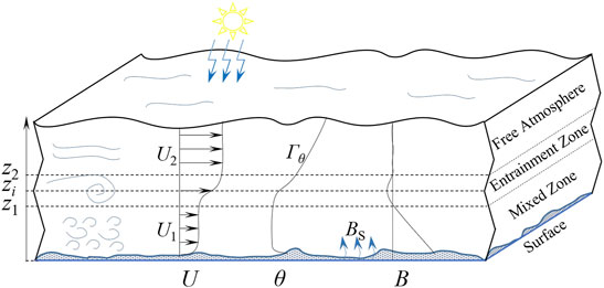
FIGURE 1. Schematic diagram of the sheared CBL and the vertical distribution of the horizontal velocity U, potential temperature θ, and buoyancy flux B. B_S is the surface buoyancy flux; Γ_θ is the potential temperature gradient of the free atmosphere; z_i, z₁, and z₂ denote the height, upper, and lower limits of the entrainment zone, respectively; z_S refers to the level of the surface; and U₁ and U₂ are the horizontal mean velocities.

A stratified saline flume is an effective platform to study the stratified and sheared CBL, which can control the governing parameters of the CBL at the laboratory scale, accurately simulate the stratified structure and turbulent flow characteristics of the CBL, and provide reliable experimental data. Willis and Deardorff (1974) simulated the stratified flow in a convection chamber and analyzed the turbulent kinetic energy (TKE) distribution in the mixed zone. The mean temperature and heat flux measured in their experiments were in good agreement with the atmospheric observations. They further studied the turbulence in the mixed zone and analyzed the turbulence spectrum and the entrainment rate in the boundary layer (Deardorff and Willis, 1985). Park, Seo and Lee (2001) investigated the diffusion characteristics of the bottom plume in a stratified experimental flume and analyzed the empirical formula of the downwind distance of the plume diffusion. Li et al. (2008) carried out the flume experiments with non-uniform heating of the underlying surface, and their results showed that the turbulent vortex structure in the mixed region was more stable and the turbulence intensity was significantly enhanced. Jonker and Jimènez (2014) used laser-induced fluorescence (LIF) to measure the salinity distribution in a stratified saline tank to simulate a shear-free CBL with medium to high Richardson numbers (Ri), analyzed the entrainment flux, and discussed the influence of the Reynolds number (Re) and the Prandtl number (Pr) on the entrainment process.

The thickness of the entrainment layer, Δz (Δz = z₂—z_i), quantifies the effect of various factors influencing the entrainment process. Deardorff et al. (Deardorff, 1980; Deardorff et al., 1980; Deardorff and Willis, 1985) measured the vertical distribution of the horizontal mean potential temperature (θ) and buoyancy flux (B) in a stratified flume without shear and found that the entrainment zone thickness Δz was about 20–40% of the mixed zone thickness. They obtained the following correlation between Δz/z_i and the bulk convective Richardson number $R{i}_{\ast }$ as follows:

$\frac{\Delta z}{z_i}=1.31R{i}_{\ast }^{-1}+0.21,(1)$

where $R{i}_{\ast }$ is defined as follows:

$R{i}_{\ast }=\frac{g}{{\theta }_0}\left(\frac{\Delta \theta z_i}{w_{\ast }^2}\right),(2)$

in which g is the acceleration due to gravity, θ₀ is the bulk temperature, Δθ is the temperature step over the entrainment zone, and $w_{\ast }$ is the characteristic convection velocity, which is defined as follows:

$w_{\ast }={\left(\frac{g}{{\theta }_0}\overline{{\left(w^{\prime }{\theta }^{\prime }\right)}_S}{z}_i\right)}^{1/3},(3)$

where $\overline{{\left(w^{\prime }{\theta }^{\prime }\right)}_S}$ is the buoyancy flux at the surface.

Sun et al. (2005) found that Δθ was proportional to the potential temperature gradient of the entrainment layer, that is, Δθ/Δz = C₁Γ_θ, where C₁ is a proportional constant, and obtained a new relation for Δz/z_i given as follows:

$\frac{\Delta z}{z_i}=C_2{\left(\frac{{\theta }_{\ast }}{{\Gamma }_{\theta }{z}_i}\right)}^{1/2}=C_2{S}^{1/2},(4)$

in which C₂ is another proportional constant, ${\theta }_{\ast }$ is the characteristic potential temperature, Γ_θ is the potential temperature gradient, and $S={\theta }_{\ast }/\left({\text{Γ}}_{\theta }{z}_i\right)$ is a dimensionless number. They believed that this relation was more consistent with the measured data of the stratified water tank experiments than the traditional $R{i}_{\ast }^{-1}$ correlation due to the inclusion of the effect of the potential temperature gradient on the entrainment process.

Jonker and Jiménez (2014) developed a saline tank with a microporous plume at the bottom to simulate the buoyancy effect and studied the entrainment characteristics of the shear-free stratified flow. Sabeghadam et al. (2017) studied the entrainment effect of the stable stratification at different Richardson numbers in a rectangular stratified water tank and proposed a simple qualitative model for the growth of the mixed zone. Their results showed that due to the omission of the shear, the proposed model produces noticeable deviations from the observational data of the atmospheric CBL.

In order to examine the influence of the velocity shear effect on the generation and evolution of the entrainment flow, Odell and Kovasznay (1971) designed a circulating water flume with two counter-rotating disk pumps that use the friction stress of multilayer impeller plates on the fluid to generate steady thrust. Narimousa, Long and Kitaigorodskii (1986), Jackson (2006), and Strang and Fernando (2010) carried out experiments using such a setup to successfully identify the fluid layers with different characteristics, which were dominated by different flow transport mechanisms, and obtained the scaling relationship for the entrainment rate in the stratified flow. Kirkpatrick et al. (Kirkpatrick and Armfield 2005; Kirkpatrick et al., 2012) built an experimental flume for a stratified saline flow, in which freshwater was driven across the saline layer to make the vertical shear, and freshwater was also injected through the micro-orifices at the bottom to simulate the buoyancy effect from the CBL surface. The velocity and density data of the flow were obtained by particle image velocimetry (PIV) and planar LIF devices.

Until now, there are still many technical problems in the experimental study of the CBL with vertical shear, especially in the simulation of the entrainment process. By modifying the experimental flume design of Kirkpatrick et al. (2012), in this study, we designed and constructed an open experimental flume with stratified fluid to simulate the comprehensive influence of shear, buoyancy, and surface buoyancy flux on the CBL entrainment process with three-dimensional velocity data of the stratified flume obtained by using a PIV device. The obtained experimental data were analyzed, which provided improved understanding of the flow characteristics. A new scaling relationship for the entrainment zone thickness was also proposed.

2 Experimental Methods

2.1 Stratified Saline Flume Apparatus

The experimental flume apparatus of CBL uses saline water and freshwater to achieve the density-stratified flow. The setup of the flume and the data acquisition device are sketched in Figure 2. The inlet part of the apparatus is a 0.15-m × 0.1-m × 0.3-m (width × height × length) diversion channel, which is divided into two 0.05-m-height rectangular channels by a horizontal partition. The built-in wire mesh can filter the water flow and evenly distribute the fluid velocity on the inlet cross-section of the flume.

FIGURE 2

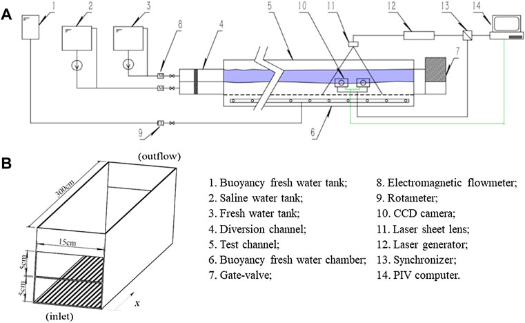
FIGURE 2. Experimental stratified flow flume setup and the PIV measurement system: (A) process flow diagram and (B) test channel structure.

The test channel with an upper opening, where the stratified flow occurs and the data are measured, was made of 3-m-long plexiglass and an array of micro-orifices with an aperture diameter of 200 μm and a spacing of 0.005 m drilled at the bottom. A 45° bend connected the drainage section and the test channel terminal, which weakens the disturbance to the horizontal section by the backflow at the gate valve. The opening of the gate valve controls the drainage of the flume to maintain the balance of the flow and the water level. The saline and freshwaters were controlled to flow in the lower and upper channels of the diversion channel and to be in a fully developed turbulent state in the test channel. By adjusting the concentration of the saline water and the velocities of the upper and lower layers, the stratified flows with different density gradients and velocity shear effects can be formed in the test channel.

The freshwater chamber was installed at the bottom of the test channel, and the inner flute-type pipe can evenly distribute the inlet water and relax the water pressure fluctuation. The freshwater vertically flowed into the lower saline layer of the test channel through the micro-orifice array in a plume shape and created the buoyancy flux on the CBL surface.

A 0.05-m-high overflow weir was set at the drainage end to maintain the lower fluid stationary (U₁ = 0), and only the upper freshwater velocity can be controlled in experiments. The density of saline was either 1,025 kg/m³ or 1,060 kg/m³, the buoyancy plume flux Q_S at the bottom was either 20 L/h (20 L/h = 5.6 × 10⁻⁶ m³/s, corresponding to the buoyancy plume velocity at the bottom of w_S = 0.0005 m/s) or 40 L/h (1.1 × 10⁻⁵ m³/s, w_S = 0.001 m/s), and the velocity difference ΔU = U₂—U₁ = U₂ was in the range of 0.01–0.15 m/s. The experimental cases and the associated parameter values are listed in Table 1. It should be noted that some cases listed in Table 1 have the same values of the control parameters (i.e., Q_s, ρ₀, and U₂) but differ in the locations to capture the camera photos and obtain the PIV data (i.e., x = 5z_i, 12z_i, 20z_i, and 36z_i, where z_i is the height of the entrainment zone); as for each experimental case, the camera photos and PIV data can only be obtained at one specific location (x).

TABLE 1

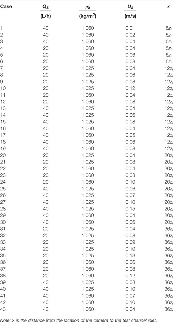
TABLE 1. Experimental cases and the associated parameter values.

2.2 Particle Image Velocimetry and Density Measurements

The experimental apparatus was equipped with the PIV device (LaVision: 3D FlowMaster Stereoscopic PIV). The beam emitted by the laser generator (Dual pluse Nd:YAG laser) passes through the lens and produces a sheet light with a thickness of 1–2 mm, 15 Hz frequency, and 532 nm wavelength in the center of the test channel to illuminate the tracer particles in the water. The tracer particles are white hollow glass beads with a size of 10 μm and a density of 1,030–1,050 kg/m³ close to the saline density in the flume. Two CCD cameras (Imager sCMOS, 1,600 × 1,200 pixels) were located on the same side of the test channel at the height of the interface between the saline water and freshwater to capture the trajectory of particles in the 0.15-m × 0.15-m plane at the same frequency as the laser beam, and the 3-D velocity data of the flow field were obtained and processed by DaVis 8.4 post-process software to describe the spatial structure and flow characteristics of the flow field accurately. Densities were measured by using a Mettler Toledo Densito 30PX Density Meter (resolution: 0.1 kg/m³, accuracy: ± 1.0 kg/m³). More details about the experimental apparatus and the PIV and density measurements can be found in Li (2020).

2.3 Characteristic Governing Parameters of the Flume

2.3.1 Test Channel Aspect Ratio, Ar

The sidewalls of the channel can limit and reflect the spanwise diffusion of the entrainment vortex and then affect its structure, which requires the geometric size of the channel to achieve a certain value of Ar (the ratio of the width of the channel to the level of the interface which is the height of the bottom saline water layer) to present ideally the entrainment process. Willis and Deardroff (1974) found that the influence of the sidewalls on the turbulence of the central flume in a tank with Ar = 2 was so large that it caused insufficient evolution of the horizontal velocity and large variance of the vertical velocity. Hadfield, Cotton and Pielke (1992) considered the influence range of the sidewalls on the central vortex within a vortex scale distance equivalent to the height of the entrainment zone z_i and suggested that at least one vortex scale space should be left on both sides of the flume, that is, the Ar of the experimental flume is at least three so as to reduce their damage on the central turbulent vortex. The test channel in our experiments with Ar = 3 can be considered that the sidewalls will not have a significant effect on the turbulence in the center flow regions.

2.3.2 Reynolds Number, Re

The test channel Reynolds number is Re_ch = U₂D_h/ν = 3,000 ∼ 11,250, and the bulk Reynolds number is Re = U₂z_i/ν = 2000 ∼ 7,500, where D_h is the hydraulic diameter and ν is the kinematic viscosity of water. The critical Re of laminar flow in an open channel is 500, so the flows in the experiments are in a fully developed turbulent state.

The buoyancy plume velocity at the bottom is w_S = 0.0005 ∼ 0.001 m/s, which is significantly smaller than $w_{\ast }$ ($w_{\ast }$ = 0.0183 ∼ 0.0309 m/s), and the Reynolds number of the buoyancy plume is Re_S = D_hw_S/ν = 0.25–0.5, which is much less than Re_ch of the horizontal flow in the test channel. Therefore, the upward movement of the buoyancy plume at the bottom has a negligible effect on the horizontal flow.

2.3.3 Richardson Number, Ri

In the entrainment zone, the buoyancy step value is Δb_e = g (ρ—ρ₀) and the bulk Richardson number is Ri = Δb_ez_i/(ΔU)² = 1.3–18.4, which is much larger than the critical value range of 0.15–0.5 for the formation of stable stratified turbulence, that is, the large velocity gradient fluctuation causes the instability of the interface disturbance wave and forms a stable entrainment zone (McGrath et al., 1997).

The convection Richardson number of the experimental flume $R{i}_{\ast }$, as defined by Eq. 2, is 12.9– 87.8, which is beyond the critical point Ri_cr = 10, corresponding to the dynamic process related to the entrainment in a stratified flow (Fedorovich et al., 2004).

2.3.4 Rayleigh Number, Ra_f

Ra_f is used to represent the relative influence of convection diffusion and concentration diffusion on the salt molecule distribution in the saline fluid. The diffusion coefficient of salt molecules is D_S = 1.33 × 10⁻⁹ m²/s, the viscosity of saline water is ν = 1 × 10⁻⁹ m²/s, and Ra_f = B_Sz_i⁴/(νD_S²) = (1.04–2.08) × 10¹⁶, which is much larger than the critical value of 10¹⁴ (Hibberd and Sawford, 1994), indicating that the effect of the salt concentration diffusion on turbulent density is very small, and the density field in a stratified flow is dominated by convection diffusion.

3 Characteristics of Stratified Flow Field

3.1 Vertical Stratification Characteristics

The upper freshwater was dyed with blue ink to enhance the layered visualization, as shown by the image presented in Figure 3 as an example, and the channel can clearly show the phenomenon of stratified flow. There is an obvious entrainment transition layer in the middle in which the color changes gradually, indicating that there is a large density gradient in the thin layer.

FIGURE 3

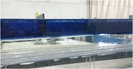
FIGURE 3. Camera photo of the experimental flume to show the stratification in the channel at the commencement of the flow for the case of Q_S = 20 L/h, U₂ = 0.08 m/s, and ρ₀ = 1,060 kg/m³ (case 6).

The freshwater beams from the bottom array, affected by the net buoyancy from the density difference, rise up into the saline layer. Due to the existence of small-scale eddy turbulence in the layer, the fluid columns do not float vertically upward and diffuse upward in curved plume.

Figure 4 presents the PIV vorticity contours at x = 12z_i away from the test channel inlet. There is an obvious extremum region at the interface of the flow field where the vorticity values are more than one order of magnitude larger than that in other regions, and the thickness of the entrainment zone can be distinguished from the vertical variation region of vorticity in the figure. It is seen that the entrainment zone thickness increases when the velocity difference is increased from 0.06 m/s to 0.08 m/s by comparing Figures 4A–C and Figures 4B–D, respectively, with the same bottom buoyancy flux and saline density; Similar changes occur as revealed by comparing Figures 4A,E,B, and F respectively, where the bottom buoyancy flux increases from 20 L/h to 40 L/h with other conditions unchanged; the gradient of the intermediate region decreases and the thickness slightly increases as demonstrated by comparing Figures 4A–F, respectively, when the density of the saline water decreases from 1,060 kg/m³ to 1,025 kg/m³. There is also a thin region with a quite larger vorticity close to the bottom, mainly due to the upwelling motion of the buoyancy plume and shear effect generated by the lower saline water and the channel floor, which makes the fluid in this region to be not fully stationary and to generate vortices, but the magnitudes are much smaller than that in the middle region.

FIGURE 4

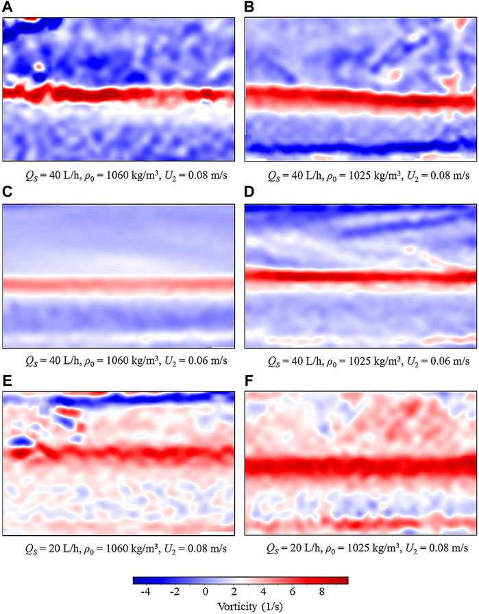
FIGURE 4. PIV snapshots of the vorticity contours of the spanwise central plane at x = 12z_i away from the test channel inlet for (A) case 19, (B) case 15, (C) case 18, (D) case 14, (E) case 12, and (F) case 9, respectively.

3.2 Horizontal Characteristics

In the experimental cases with Q_S = 40 L/h and ρ₀ = 1,060 kg/m³, the upper freshwater flows above the saline layer at the velocity of U₂, and the streamline data at x = 5z_i away from the inlet captured by PIV are compared in Figure 5. When U₂ = 0.01 m/s, as shown in Figure 5A, the shear stress at the interface is not strong enough to overcome the molecular viscous force to form an entrainment vortex, which only causes the oscillation of the interface. The increase in U₂ to 0.02 m/s intensifies the oscillation of the interface, making the interface to become blurred with the twist of streamlines, as shown in Figure 5B. Until U₂ attains about 0.04 m/s, a distinguishable clockwise entrainment vortex appears at the interface, as shown in Figure 5C. According to the data under this condition, the bulk convective Richardson number $R{i}_{\ast }$ = Δb_ez_i/ $w_{\ast }^2$ = 7.85 ($w_{\ast }$ is calculated using Eq. 3). Because the flow field is too close to the inlet to form a stable entrainment vortex, the proportion of TKE produced by shear to promote entrainment should be less than the coefficient of ΔU in Eq. 6 of 0.4. Therefore, the actual value of $R{i}_{\ast }$ should be slightly greater than 7.85, which is in accordance with Ri_cr = 10 at the transition point of the CBL (Fedorovich et al., 2004).

FIGURE 5

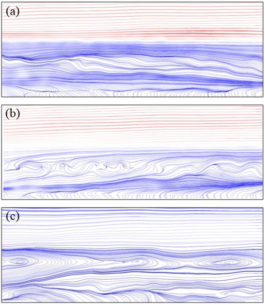
FIGURE 5. PIV snapshots of the streamlines on the central plane at x = 5z_i away from the inlet at different values of U₂ with Q_S = 40 L/h and ρ₀ = 1,060 kg/m³: (A) U₂ = 0.01 m/s (case 1), (B) U₂ = 0.02 m/s (case 2), and (C) U₂ = 0.04 m/s (case 3), respectively.

Figure 6 presents the PIV-produced streamline views on the central plane at x = 12z_i away from the inlet for the cases of Q_S = 20 L/h and ΔU = 0.08 m/s with ρ₀ = 1,025 kg/m³ and 1,060 kg/m³ (cases 9 and 12), respectively. It can be seen that the vortex was the main flow structure in the middle region, and the vortex was elongated in the flow direction due to the shear effect and density gradient at the interface. The maximum width of the vortex is about (1.0–1.5)z_i. Due to the limitation of buoyancy, the vortex was finally confined in the middle thin layer, and then gradually developed into a stable entrainment zone.

FIGURE 6

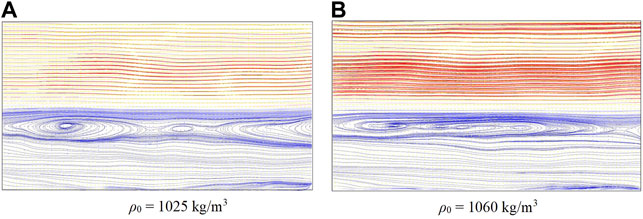
FIGURE 6. PIV snapshots of the streamlines on the spanwise central plane at x = 12z_i from the test channel inlet for the cases of Q_S = 20 L/h and U₂ = 0.08 m/s with, (A) ρ₀ = 1,025 kg/m³ (case 9), and (B) ρ₀ = 1,060 kg/m³ (case 12), respectively.

3.3 Horizontal Velocity Profile

It can be seen from the aforementioned analysis that a stable intermediate entrainment zone appeared at the interface after about 12z_i from the inlet. Figure 7 presents the vertical profiles of the horizontal mean velocity component recorded at 20z_i with different values of saline density, buoyancy flux, and velocity difference. It is found that the horizontal velocity remained constant in the main regions of the lower and upper layers but changed gradually with large rates in the intermediate layer. The large variations of the horizontal velocity profile within the intermediate layer clearly showed that the control parameters of the flows have significant influences.

FIGURE 7

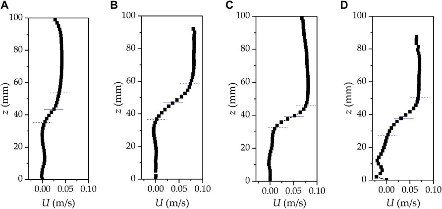
FIGURE 7. Vertical profiles of the horizontal velocity at x = 20z_i under different values of the control parameters of the flows: (A) case 20, (B) case 21, (C) case 22, and (D) case 23, respectively. The dashed lines represent the upper and lower limits of the entrainment zone, and the solid line is the height of the entrainment zone.

3.4 Thickness of the Entrainment Zone

The entrainment zone of the stratified flow is defined by the vertical profile of the horizontal velocity obtained from the experiment, as shown in Figure 7, where z_i corresponds to the level of the maximum gradient, the lower and upper height limits z₁ and z₂ are the heights with zero velocity gradients, and the thickness is Δz = z₂—z_i. However, there is a large fluctuation of the upper interface of the entrainment zone in the experiments, which makes it difficult to determine the height of the velocity gradient of zero accurately. In order to reduce the measurement errors, as an approximation, Δz is taken as the height range from 10 to 90% of U₂.

By comparing Figures 7A,B it is seen that the increase in U₂ from 0.04 m/s to 0.08 m/s enhances the shear at the interface, which makes more shear-generated TKE consumed by the entrainment process and Δz increases. The increase in the saline water concentration enhances the density gradient of the entrainment zone, and the viscosity force of parcels close to the interface exceeds the shear stress prematurely, which makes the entrainment vortex to break up when it does not grow enough. Meanwhile, the entrainment process is limited, and Δz decreases as shown in Figures 7A,C. Similarly, when ρ₀ and U₂ do not change, the increase in the bottom buoyant flux promotes more buoyant freshwater to intrude into the entrainment zone, which is equivalent to dilute the density gradient in the region, and accordingly, Δz increases as shown in Figures 7B,D.

3.5 Counter-Gradient Transport of Momentum

The turbulent entrainment process in the sheared CBL results from the combined effects of shear stress and buoyancy. Vortices in different scales generated in the entrainment zone transport the high-density parcels from CBL to the upper free atmosphere with low density, that is, the counter-gradient transport process. The vertical TKE governing equation of CBL is as follows:

$\frac{\partial \overline{k}}{\partial t}=-\left(\overline{u^{\prime }{w}^{\prime }}\frac{\partial U}{\partial z}+\overline{v^{\prime }{w}^{\prime }}\frac{\partial V}{\partial z}\right)+\frac{g}{{\theta }_0}\overline{w^{\prime }{\theta }^{\prime }}-\frac{\partial \overline{w^{\prime }{k}^{\prime }}}{\partial z}-\frac{1}{{\rho }_0}\frac{\partial \overline{w^{\prime }{p}^{\prime }}}{\partial z}-\epsilon ,(5)$

where $\overline{k}=\frac{1}{2}\left(\overline{u^{,2}}+\overline{v^{,2}}+\overline{w^{,2}}\right)$ is the average TKE; ε is the dissipation rate of turbulent energy; $u^{\prime }$, $v^{\prime }$, and $w^{\prime }$ are the fluctuations of the velocity components; and $p^{\prime }$ is the fluctuation of the local atmospheric pressure.

Once the shear term of TKE equation satisfies $-\overline{u^{\prime }{w}^{\prime }}\frac{\partial U}{\partial z}<0$, the velocity gradient is opposite to the Reynolds stress direction and the momentum is transported in the counter-gradient direction. Figure 8 shows the vertical profiles of the momentum transport under different experimental conditions. The results show that the momentum transport term in the saline layer fluctuates weakly because the region is subjected to small-scale vortex turbulent mixing effect and −∂U/∂z is approximately zero. A negative peak in the middle region indicates that the Reynolds stress is opposite to the velocity gradient and the TKE is dissipated. The peak value increases under the conditions of strong stratification and strong shear, indicating that more TKE is consumed by shear in the entrainment zone.

FIGURE 8

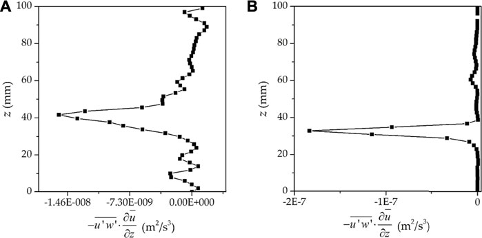
FIGURE 8. Vertical profiles of the shear term of the TKE equation under different experimental conditions: (A) case 7 and (B) case 12, respectively.

4 Parameterization of the Entrainment Zone Thickness

4.1 Characteristic Velocity Scale

The CBL entrainment process is affected by both buoyancy and shear (see Eq. 1), and the characteristic velocity of the flow field should not only include buoyancy term but also reflect the influence of the velocity shear effect. A proportion of the shear-generated TKE is used to promote the entrainment process, and the rest is dissipated by the molecular viscosity. The shear-generated TKE at the surface is dissipated in a short distance from the bottom, which has little effect on the entrainment process (Conzemius and Fedorovich, 2006a, 2006b; Haghshenas and Mellado, 2019); therefore, it will not make a large error to neglect this part in the parameterization of the entrainment zone thickness.

Assuming that the effects of buoyancy and shear on entrainment are independent of each other; the scale of the characteristic convective velocity in the sheared CBL is represented as follows:

$w_m^2=w_{\ast }^2+C_3\left(\Delta U^2+\Delta V^2\right),(6)$

where C₃ is the fraction of the shear-generated TKE consumed by the entrainment process, which is in the range of 0.38–0.43 with the mean value of 0.4 (Liu et al., 2016a; Liu et al., 2016b; Li et al., 2020), and ΔU and ΔV are the steps of the horizontal velocity components in the entrainment zone, which represent the velocity shear effects on the entrainment. In this study, ΔV = 0 as there is no shear in the V-direction.

4.2 Theoretical Parametric Model

The buoyancy flux from the surface heats the air parcels in the adjacent area to generate buoyancy, and the parcels float up into the free atmosphere. The buoyancy decreases to zero at z_i where the velocity reaches the maximum w_m, as depicted in Figure 1. Due to the influence of inertia, the parcels move upward in the region of z_i ∼ z₂ to overcome the negative buoyancy. The thickness of the entrainment zone is related to the work of negative buoyancy when the parcels move above the intermediate buoyancy level in the parcel theory. The energy conservation relation of the process is given as follows:

$0-\frac{1}{2}{w}_m^2=\underset{z_i}{\overset{z_2}{{\displaystyle \int }}}\frac{\left(\rho -{\rho }_0\right)}{{\rho }_0}gdz.(7)$

The density variation is mainly caused by the change of potential temperature. The atmosphere can be treated as an incompressible fluid, and the effect of pressure on density can be ignored in the limited thickness of CBL. The Boussinesq approximation gives the following expression:

$\frac{d\rho }{dz}=-\beta {\rho }_0\frac{d\theta }{dz},(8)$

where β is the thermal expansion coefficient of fluid. Sun et al. (2005); Sun (2009) found the following linear relation of the temperature gradient between the entrainment zone and the free atmosphere:

$\frac{d\theta }{dz}=C_4{\text{Γ}}_{\theta },(9)$

where C₄ is a constant. Combining Eq. 8 and 9, Eq. 7 can be written as follows:

$-\frac{1}{2}{w}_m^2=0-\frac{C_4}{2}\beta {\rho }_{0}g{\Gamma }_{\theta }\text{Δ}{z}^2,(10)$

that is,

$\frac{\text{Δ}z}{z_i}={\left(\frac{C_4{\rho }_{0}g\beta {\text{Γ}}_{\theta }{z}_i^2}{w_m^2}\right)}^{-1/2}=C_{5}R{i}_{NC}^{-1/2},(11)$

in which C₅ is a proportional constant and Ri_NC = N²z_i²/w_m² is the corrected bulk Richardson number, where N² is the buoyancy frequency defined as follows:

$N^2=-\frac{g}{{\rho }_0}\frac{d\rho }{dz}=C_{4}g\beta {\Gamma }_{\theta }.(12)$

4.3 Experimentally Quantified Scaling Relation Between Δz/z_i and Ri_NC

The scaling relation between Δz/z_i and Ri_NC was quantified using the experimental data of the cases listed in Table 1. As shown in Figure 9A, the experimental results give the following quantified scaling relation:

$\frac{\text{Δ}z}{z_i}=1.17R{i}_{NC}^{-1/2}.(13)$

FIGURE 9

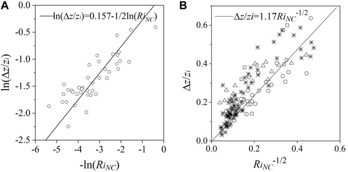
FIGURE 9. Scaling relation between the dimensionless thickness of entrainment zone Δz/z_i and Ri_NC. ○ experimental data of this study; ✳ radar data from Boers and Eloranta (1986);□ radar data from Lothon et al. (2008); △ large eddy simulation data of Otte and Wyngaard (2001); — linear fit of the experimental data of this study.

The performance of this quantified scaling relation was further examined by comparing its predictions to the numerically simulated data of Otte and Wyngaard (2001) and the radar measurement data of Boers and Eloranta (1986) and Lothon, Lenschow and Mayor (2008), with the result presented in Figure 9B. It is seen that this new scaling relation based on the stratified saline experiments is consistent with the available data and is able to predict the thickness of the entrainment zone in the stratified CBL with vertical velocity shear relatively accurately.

4.4 Error Analysis

The upper freshwater layer of the stratified saline flume apparatus adopted uniform fluid, which was different from the actual CBL which had a small density gradient (temperature gradient) in the upper layer. However, the entrainment process occurs at the interface of the two fluids, and the fluid parameters at the sufficient height of the upper layer do not affect the material exchange in the entrainment layer. Therefore, it is acceptable to use the fluid with constant density to simulate the sheared CBL, which has little effect on the entrainment process.

The bottom buoyancy plume diluted the saline water, weakened the actual buoyancy effect, and lifted the level of the saline layer. The freshwater from the microporous bottom had an effect on the saline concentration in the test channel by about 0.17–0.73% during the experiment period of 5 min which affected the entrainment zone height z_i by about 3.7–7.4% assuming that the buoyancy plume volume promotes an overall uplift of the saline layer. The comprehensive influence of these two factors on the coefficient (i.e., 1.17) of Eq. 13 is about 1.25–2.55% deviation, of which the uplift of the saline layer is a greater one because of the addition of buoyant freshwater. Therefore, using a larger Ar of the test channel and shortening the experiment period are conducive to reduce the errors.

It is unavoidable that there were certain deviations of the apertures of the micro-orifice array in the manufacturing process, which led to an inhomogeneous distribution of the buoyancy plume in the surface. In addition, the friction effect of the channel sidewalls and the influence of the backflow at the terminal sluice made the stratified flow slightly different from the conditions analyzed.

5 Conclusion

A stratified saline flume experimental apparatus was designed to simulate the stratified flow of the CBL with vertical velocity shear, and the PIV device was used to capture the 3-D velocity field data. The flow field characteristics and the entrainment zone thickness with different control parameter values were experimentally studied.

The experimental setup shows a significant stratification of the saline and freshwater and the formation, development, and breakup process of the entrainment vortices. When the velocity difference between the upper and lower layers is only 0.01 m/s, the velocity shear is too weak to overcome the viscous force to form an entrainment vortex. The vortex with the characteristic length about (1.0–1.5)z_i can be observed at the test channel inlet until the velocity difference increases up to 0.04 m/s, and a stable middle entrainment zone is formed after about 12z_i from the inlet with an counter-gradient momentum transport process.

The entrainment zone is defined by the horizontal velocity gradient, and its thickness Δz is obviously affected by the bottom buoyancy flux, the velocity difference, and the density difference, with the first two promoting the growth of the entrainment zone, while the last being able to increase the density gradient of the middle interface to hinder the entrainment process.

Based on the experimental data, a new quantified scaling relation between the dimensionless thickness of the entrainment zone and the corrected Richardson number is established, that is, Δz/z_i = 1.17Ri_NC^−1/2, and the analysis of the experimental errors suggests that a larger aspect ratio flume is helpful to improve the accuracy of the experimental results. The effectiveness of the proposed model is verified by the available radar test data and numerical simulation data, and it is found that it can well predict the entrainment zone thickness of the sheared CBL.

Data Availability Statement

The original contributions presented in the study are included in the article/Supplementary Material, further inquiries can be directed to the corresponding authors.

Author Contributions

WG and WL contributed to the overarching research goals and technical route; AL and WG performed the experiments; AL, WG and WL contributed significantly to the analysis of the experimental results; AL prepared the manuscript draft and WL provided the revision; and TL and YX helped to conduct the experiments.

Funding

This research was funded by the National Natural Science Foundation of China (grant numbers 51969032 and 51866016).

Conflict of Interest

The authors declare that the research was conducted in the absence of any commercial or financial relationships that could be construed as a potential conflict of interest.

Publisher’s Note

All claims expressed in this article are solely those of the authors and do not necessarily represent those of their affiliated organizations, or those of the publisher, the editors, and the reviewers. Any product that may be evaluated in this article, or claim that may be made by its manufacturer, is not guaranteed or endorsed by the publisher.

References

Allaerts, D. (2016). Large-eddy Simulation of Wind Farms in Conventionally Neutral and Stable Atmospheric Boundary Layers. Belgium: PhD ThesisKU Leuven.

Google Scholar

Boers, R., and Eloranta, E. W. (1986). Lidar Measurements of the Atmospheric Entrainment Zone and the Potential Temperature Jump across the Top of the Mixed Layer. Boundary-layer Meteorol. 34 (4), 357–375. doi:10.1007/bf00120988

CrossRef Full Text | Google Scholar

Conzemius, R. J., and Fedorovich, E. (2006a). Dynamics of Sheared Convective Boundary Layer Entrainment. Part I: Methodological Background and Large-Eddy Simulations. J. Atmos. Sci. 63 (4), 1151–1178. doi:10.1175/jas3691.1

CrossRef Full Text | Google Scholar

Conzemius, R. J., and Fedorovich, E. (2006b). Dynamics of Sheared Convective Boundary Layer Entrainment. Part II: Evaluation of Bulk Model Predictions of Entrainment Flux. J. Atmos. Sci. 63 (4), 1179–1199. doi:10.1175/jas3696.1

CrossRef Full Text | Google Scholar

Deardorff, J. W. (1980). Stratocumulus-capped Mixed Layers Derived from a Three-Dimensional Model. Boundary-layer Meteorol. 18 (4), 495–527. doi:10.1007/bf00119502

CrossRef Full Text | Google Scholar

Deardorff, J. W., and Willis, G. E. (1985). Further Results from a Laboratory Model of the Convective Planetary Boundary Layer. Boundary-layer Meteorol. 32 (3), 205–236. doi:10.1007/bf00121880

CrossRef Full Text | Google Scholar

Deardorff, J. W., Willis, G. E., and Stockton, B. H. (1980). Laboratory Studies of the Entrainment Zone of a Convectively Mixed Layer. J. Fluid Mech. 100, 41–64. doi:10.1017/s0022112080001000

CrossRef Full Text | Google Scholar

Fedorovich, E., Conzemius, R., and Mironov, D. (2004). Convective Entrainment into a Shear-free, Linearly Stratified Atmosphere: Bulk Models Reevaluated through Large Eddy Simulations. J. Atmos. Sci. 61 (3), 281–295. doi:10.1175/1520-0469(2004)061<0281:ceiasl>2.0.co;2

CrossRef Full Text | Google Scholar

Hadfield, M. G., Cotton, W. R., and Pielke, R. A. (1992). Large-eddy Simulations of Thermally Forced Circulations in the Convective Boundary Layer. Part II: The Effect of Changes in Wavelength and Wind Speed. Boundary-layer Meteorol. 58 (4), 307–327. doi:10.1007/bf00120235

CrossRef Full Text | Google Scholar

Haghshenas, A., and Mellado, J. P. (2019). Characterization of Wind-Shear Effects on Entrainment in a Convective Boundary Layer. J. Fluid Mech. 858, 145–183. doi:10.1017/jfm.2018.761

CrossRef Full Text | Google Scholar

Hibberd, M. F., and Sawford, B. L. (1994). Design Criteria for Water Tank Models of Dispersion in the Planetary Boundary Layer. Bound.-Layer Meteorol. 67 (1-2), 97–118. doi:10.1007/bf00705509

CrossRef Full Text | Google Scholar

Jackson, P. R. (2006). Differential Diffusion of Scalars in Sheared, Stratified Turbulence. PhD Thesis. Urbana: University of Illinois at Urbana-Champaign.

Google Scholar

Jonker, H. J. J., and Jiménez, M. A. (2014). Laboratory Experiments on Convective Entrainment Using a saline Water Tank. Boundary-layer Meteorol. 151 (3), 479–500. doi:10.1007/s10546-014-9909-3

CrossRef Full Text | Google Scholar

Kirkpatrick, M. P., and Armfield, S. W. (2005). Experimental and Large Eddy Simulation Results for the Purging of Salt Water from a Cavity by an Overflow of Fresh Water. Int. J. Heat Mass Transfer 48, 341–359. doi:10.1016/j.ijheatmasstransfer.2004.08.016

CrossRef Full Text | Google Scholar

Kirkpatrick, M. P., Starner, S. H., Williamson, N., and Armfield, S. W. (2012). A New Experimental Rig for Investigations of Sheared Convective Boundary Layers. Launceston, Australia: 18th Australasian Fluid Mechanics Conference, 3–7.

Google Scholar

Li, A., Gao, W., and Liu, T. (2020). Contribution of Wind Shear to the Entrainment Process of the Atmospheric Convective Boundary Layer. Terr. Atmos. Ocean. Sci. 31 (3), 351–358. doi:10.3319/tao.2020.02.11.01

CrossRef Full Text | Google Scholar

Li, A. (2020). Investigation on the Entrainment Characteristics of Sheared Convective Boundary Layer in the Atmosphere environmentPhD Thesis. Kunming: Yunnan Normal University.

Google Scholar

Li, Z., Sun, J., Yuan, R., and Luo, T. (2008). A Laboratory Study on the Turbulent Characteristics of Convective Boundary Layer Driven by Heterogeneous Surface Heating. J. Nanjing Uni. (Natural Sci. 44 (6), 575–582. (in Chinese).

Google Scholar

Liu, P., Sun, J., and Shen, L. (2016a). Parameterization of Sheared Entrainment in a Well-Developed CBL. Part I: Evaluation of the Scheme through Large-Eddy Simulations. Adv. Atmos. Sci. 33 (10), 1171–1184. doi:10.1007/s00376-016-5208-x

CrossRef Full Text | Google Scholar

Liu, P., Sun, J., and Shen, L. (2016b). Parameterization of Sheared Entrainment in a Well-Developed CBL. Part II: A Simple Model for Predicting the Growth Rate of the CBL. Adv. Atmos. Sci. 33 (10), 1185–1198. doi:10.1007/s00376-016-5209-9

CrossRef Full Text | Google Scholar

Lothon, M., Lenschow, D. H., and Mayor, S. (2008). Measurements of Turbulence Structure in the Daytime Convective Boundary Layer from a Ground-Based Doppler Lidar in. 18th Symposium on Boundary Layers and Turbulence. Stockholm, Sweden. 7B.1.

Google Scholar

McGrath, J. L., Fernando, H. J. S., and Hunt, J. C. R. (1997). Turbulence, Waves and Mixing at Shear-free Density Interfaces. Part 2. Laboratory Experiments. J. Fluid Mech. 347, 235–261. doi:10.1017/s0022112097006526

CrossRef Full Text | Google Scholar

Narimousa, S., Long, R. R., and Kitaigorodskii, S. A. (1986). Entrainment Due to Turbulent Shear Flow at the Interface of a Stably Stratified Fluid. Tellus 38A (1), 76–87. doi:10.1111/j.1600-0870.1986.tb00454.x

CrossRef Full Text | Google Scholar

Odell, G. M., and Kovasznay, L. S. G. (1971). A New Type of Water Channel with Density Stratification. J. Fluid Mech. 50 (3), 535–543. doi:10.1017/s002211207100274x

CrossRef Full Text | Google Scholar

Otte, M. J., and Wyngaard, J. C. (2001). Stably Stratified Interfacial-Layer Turbulence from Large-Eddy Simulation. J. Atmos. Sci. 58 (22), 3424–3442. doi:10.1175/1520-0469(2001)058<3424:ssiltf>2.0.co;2

CrossRef Full Text | Google Scholar

Park, O. H., Seo, S. J., and Lee, S. H. (2001). Laboratory Simulation of Vertical Plume Dispersion within a Convective Boundary Layer. Boundary-Layer Meteorology 99 (1), 159–169. doi:10.1023/a:1018731205971

CrossRef Full Text | Google Scholar

Sabetghadam, S., Khoshsima, M., and Bidokhti, A. A. (2017). Simulation of Entrainment Near a Density Stratified Layer: Laboratory experiment and LIDAR Observations. J. Earth Space Phys. 42 (4), 27–34.

Google Scholar

Strang, E. J., and Fernando, H. J. S. (2010). Vertical Mixing and Transports through a Stratified Shear Layer. J. Phys. Oceanogr. 31, 2026–2048.

Google Scholar

Sun, J., Jiang, W., Chen, Z., and Yuan, R. (2005). Parameterization for the Depth of the Entrainment Zone above the Convectively Mixed Layer. Adv. Atmos. Sci. 22, 114–121.

Google Scholar

Sun, J. (2009). On the Parameterization of Convective Entrainment: Inherent Relationships Among Entrainment Parameters in Bulk Models. Adv. Atmos. Sci. 26 (5), 1005–1014. doi:10.1007/s00376-009-7222-8

CrossRef Full Text | Google Scholar

Willis, G. E., and Deardorff, J. W. (1974). A Laboratory Model of the Unstable Planetary Boundary Layer. J. Atmos. Sci. 31, 1297–1307. doi:10.1175/1520-0469(1974)031<1297:almotu>2.0.co;2

CrossRef Full Text | Google Scholar