 Fangyi Zong
 Shugang Zhang
 Ping Chen
 Lipeng Yang2
95% of researchers rate our articles as excellent or good
Learn more about the work of our research integrity team to safeguard the quality of each article we publish.
Find out more
ORIGINAL RESEARCH article
Front. Environ. Sci. , 04 April 2022
Sec. Atmosphere and Climate
Volume 10 - 2022 | https://doi.org/10.3389/fenvs.2022.856289
This article is part of the Research Topic Extreme Events and Their Spatiotemporal Variability over Polar Regions View all 9 articles
The dual-polarized ratio (DPR) algorithm is a new algorithm that enable calculation of Arctic sea ice concentration from the 36.5-GHz channel of the sensor Advanced Microwave Scanning Radiometer for EOS/Advanced Microwave Scanning Radiometer 2 (AMSR-E/AMSR2). In this paper, we demonstrate results that the sea ice concentration data using DPR algorithm (DPR-AMSR) are evaluated and compared with other eight Arctic sea ice concentration data products with respect to differences in sea ice concentration, sea ice area, and sea ice extent. On a pan-Arctic scale, the evaluation results are mostly very similar between DPR-AMSR and the bootstrap algorithm from AMSR-E/AMSR2 (BT-AMSR), the bootstrap algorithm from SSM/I or SSMIS (BT-SSMI), the ARTIST Sea Ice algorithm from AMSR-E/AMSR2 (ASI-AMSR), and the enhanced NASA Team algorithm from AMSR-E/AMSR2 (NT2-AMSR). Among of these products, the differences in sea ice concentration agree within ±5%. However, European Space Agency Climate Change Initiative algorithm from AMSR-E/AMSR2 (SICCI-AMSR), the European Organisation for the Exploitation of Meteorological Satellites Ocean and Sea Ice Satellite Application Facility from SSM/I or SSMIS (OSI-SSMI), the ARTIST Sea Ice algorithm from SSM/I or SSMIS (ASI-SSMI), and the NASA Team algorithm from SSM/I or SSMIS (NT1-SSMI) are all lower than DPR-AMSR at sea ice edge. And NT1-SSMI had the largest negative difference, which was lower than -15% or even 20%.The difference of sea ice area was consistently within ±0.5 million km2 between DPR-AMSR and BT-AMSR, BT-SSMI, ASI-AMSR, and NT2-AMSR in all years. The smallest difference was with BT-SSMI (less than 0.1 million km2), whereas the largest difference was with NT1-SSMI (up to 1.5 million km2). In comparisons of sea ice extent, BT-AMSR, NT1-SSMI, and NT2-AMSR estimates were consistent with that of DPR-AMSR and were within ±0.5 million km2. However, differences exceeded 0.5 million km2 between DPR-AMSR and the other data sets. When ship-based visual observation (OBS) values ranged from 85% to 100%, the difference between DPR-AMSR and OBS was less than 1%. There were relatively large differences between DPR-AMSR and OBS when OBS values were less than 85% or were recorded during the summer, although those differences were also within 10%.
Because sea ice and snow have high albedo to solar radiation, they reduce heat exchange between ocean and atmosphere, and thus, sea ice has a critical role in the global climate system (Chi et al., 2019). Arctic sea ice has undergone rapid changes in the past few decades, with minimum sea ice coverage decreasing at a rate of 12.8% ± 2.3% per decade in summer (Meredith et al., 2019). Simulated results based on the Coupled Model Intercomparison Project 5 show that there will be ice-free periods in the Arctic summer during 2041–2060 (Laliberté et al., 2016). Rapid changes in Arctic sea ice area and extent have significant effects on multi-year ice, annual ice, young ice (generally less than 30 cm thick), open water, and sea ice velocity (Lei et al., 2020). In addition, rapid changes in Arctic sea ice are associated with increasing numbers of extreme weather events in the middle latitudes of the Northern Hemisphere, including increased frequency of heat waves in summer and extreme cold in winter (Graham et al., 2017). Therefore, the continuous acquisition of long-term sea ice information in the Arctic is highly significant in studying the climate of internal changes and external forcings.
Many ways are currently used to monitor Arctic sea ice, including ships, buoys, aircraft, and satellites. Scientists can directly and systematically observe sea ice of Arctic by ship, but this approach is greatly limited in time and space. Multiple observation instruments, such as a high-resolution camera, synthetic aperture radar, radiometer, scatterometer, and altimeter, can also be installed on aircraft to observe sea ice, which can provide information on changes in sea ice within a certain space range. However, those types of observations depend on aircraft trajectory and are also relatively expensive. Visible spectral remote sensing can provide high-resolution images, but this method can only monitor sea ice in daylight under a clear sky (Kern et al., 2020). However, clouds often cover most of the Arctic region, and there is also the polar night phenomenon; therefore, it is very difficult to monitor sea ice by visible spectral remote sensing (Pichel et al., 2003). Passive microwave remote sensing is superior to visible spectral remote sensing in two aspects. First, atmospheric influence on microwave radiation is relatively small in some microwave frequency channels, and thus, microwaves are almost unaffected when penetrating thick clouds at those frequency channels. Second, microwaves are radiation emitted by sea ice itself without dependence on light (Comiso et al., 2003). As a result, long-term and large-scale changes in sea ice have only been monitored by passive microwave remote sensing technology of satellites, and such observations covering more than 40 years. At present, they provide large amounts of valuable data to study sea ice–ocean–atmosphere interactions in polar regions.
Since 1972, a series of passive microwave data from satellites (such as SMMR, SSM/I, SSMIS, and AMSR-E/AMSR2) have been widely used in sea ice monitoring, as shown in Table 1. Compared with other passive microwave sensors, the AMSR-E/AMSR2 has greatly improved spatial resolution. The two sensors can also monitor some key sea ice features (such as sea ice lead, and polynya) by using 6.925-, 10.65-, and 89.0-GHz channels (Lavergne et al., 2019).
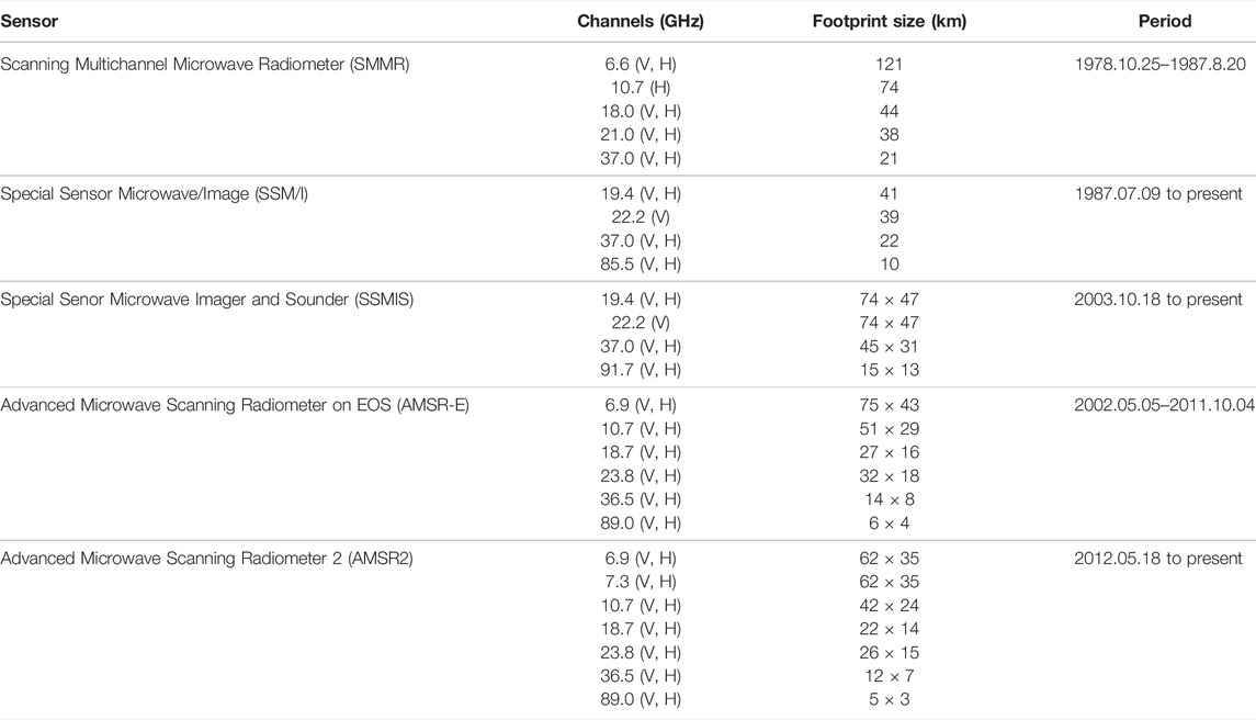
TABLE 1. Overview of multichannel passive microwave radiation satellite sensors, including vertical (V) and horizontal (H) polarization.
Since Serreze et al. (2003) reported a historical minimum in sea ice extent in September 2002; the minimum value has continued to decrease. In 2007, 2012, 2016, 2019, and 2020, sea ice extent in September reached the lowest level on record. The smallest sea ice extent was recorded in 2012 (Gascard et al., 2019). Therefore, AMSR-E/AMSR2 can be used to more accurately monitor recent changes in sea ice. Sea ice concentration is the fraction of a given area covered with sea ice and is one of the most important polar parameters not only for ocean study but also for climate study (Wayand et al., 2019). It is often retrieved from passive microwave data. At present, more than 30 sea ice concentration algorithms have been developed using passive microwave brightness temperature, and they have been subjected to much evaluation and comparison.
Accuracy and precision serve as measures of performance of a sea ice concentraiton algorithm or product. Accuracy (expressed by root mean square error, RMS) is the range, within which are the repeated retrievals of the same quantity scatter around the mean value. Precision (expressed by bias) is the difference between the mean retrieval and the true value. The NASA Team (NT) algorithm and the bootstrap (BT) algorithm, two commonly used algorithms, retrieve an average accuracy of sea ice concentration within ±5% in high-concentration ice pack during winter (Cavalieri et al., 1984; Comiso, 1986). Accuracy of the BT-AMSR algorithm is 2.5% when standard deviation of the scatter is around the ice line (Comiso, 2009). Spreen et al. (2008) compared results of the ARTIST Sea Ice (ASI) algorithm with those of NT2 and BT algorithms and found the difference between ASI and NT2 was less than −2% ± 8%, whereas that between ASI and NT was −1.7% ± 10.8%. Andersen et al. (2007) validated and compared seven sea ice concentration algorithms using reliable synthetic aperture radar data and ship-based observations data in the Arctic and found precision between 3% and 5%. However, accuracy of different sea ice concentration algorithms can be as low as ±20% during summer and along the ice edge (Meier and Notz, 2010). In addition, Ivanova et al. (2014) compared 11 sea ice concentration algorithms in the Arctic and found differences of 2%–25% for consolidate sea ice areas in winter, 5%–12% for intermediate sea ice concentration areas in winter, 2%–8% in summer, and that exceeded 12% in the Canadian Archipelago area in summer. Kern et al. (2019) evaluated and compared ten global sea ice concentration products at 12.5–50.0-km grid resolution for both the Arctic and the Antarctic, and then, they grouped the products according to observed interproduct consistency and differences in intercomparison results. All these study showed that there is no one superior algorithm, or a combination of algorithms takes advantages of each algorithm. Furthermore, GCOS (Global Observing System for Climate) requires accuracy of sea ice concentration to be within 5%, unfortunately there is no one sea ice concentration products that can provide accurate sea ice concentration for studies of the global climate system. Thus, the development of the global climate model (or the global ocean model) impels many scientific institutions and researchers continuously to develop new sea ice algorithms (or improve existing sea ice concentration algorithms) through new methods and new technologies. For example, Chi et al. (2019) applies deep learning (DL) to retrieve Arctic sea ice concentration from AMSR2 data, and Laverge et al. (2019) improve existing algorithm to retrieve sea ice concentration.
Because of distinct differences in emissivity between water and ice, most sea ice concentration algorithms apply linear combinations of passive microwave brightness temperatures at different frequencies and polarizations to distinguish sea ice from open water (Chi et al., 2019). An essential parameter for most sea ice concentration algorithms is a set of tie points, which are typical brightness temperature points for open water (0% sea ice concentration) and 100% ice coverage (100% sea ice concentration). In early sea ice concentration algorithms, including BT, NT1, NT2, and ASI algorithms, the brightness temperature tie points are usually fixed.
Brightness temperature tie points may have a range of variability for 100% sea ice coverage and open water owing to varying emissivity of sea ice, atmospheric conditions, and sea ice temperature of the emitting layer. Thus, the values of sea ice concentration are greater than or less than 100% sea ice concentration near tie points (Ivanova et al., 2015). According to Willmes et al. (2014), a dynamic technique to retrieve tie points is very advantageous when retrieving sea ice concentration using algorithms. Spreen et al. (2008) obtained greater insight into seasonal and regional stability of tie points in the ASI algorithm, but they did not use dynamic tie points and instead used fixed ones during retrieval of sea ice concentration in polar regions. In the ECICE (Environment Canada’s Ice Concentration Extractor) algorithm, the input is 100 probability distributions of brightness temperature, which are randomly and simultaneously selected, and then, optimal solutions for sea ice concentration are obtained (Shokr et al., 2008). Therefore, the key to improving accuracy of sea ice concentration algorithms is not only to determine the tie points but also to determine their seasonal and regional variations.
The dual-polarized ratio (DPR) algorithm is a new algorithm that enables calculation of Arctic sea ice concentration from the 36.5-GHz channel of the sensor (AMSR-E/AMSR2). The DPR algorithm can retrieve Arctic sea ice concentration from AMSR-E/AMSR data and was first developed using vertically and horizontally polarized brightness temperatures at the same channel of 36.5 GHz (Zhang et al., 2013; Zhang et al., 2018). With this algorithm, first, sea ice temperature of the emitting layer cannot directly influence the value of sea ice concentration; and second, sea ice concentration depends only on the ratio of dual-polarized emissivity of sea ice. Zhang et al. (2013) originally determined a fixed ratio of dual-polarized emissivity of sea ice to retrieve the whole-Arctic sea ice concentration. A dynamic ratio was then used in the DPR algorithm to improve estimation of sea ice concentration in summer and in marginal ice zones (Zhang et al., 2018). Originally, DPR algorithm’s result are compared and evaluated by the results of ABA algorithm, NT2 algorithm, ASI algorithm and MODIS optical data in some regional of Arctic. Their study showed that the sea ice concentration of DPR algorithm is improved in ice edge and in summertime in the regional experiment. However, more systematic and detailed evaluations of DPR algorithm’s results in the Arctic are not done by researchers, although this work is very important for the application of DPR algorithm in the global climate model (or the global ocean model, or regional climate impact model) in future. Thus, in this paper we evaluate and compare DPR algorithm’s results with others sea ice concentration products, which are popularly (or commonly) used in climate (or ocean) research.
In this paper, the sea ice concentration product of the DPR algorithm (DPR-AMSR) was retrieved according to Zhange et al., 2018. In Section 3, development of the DPR algorithm is detailed, and others sea ice concentration algorithms are also simply introduced. Then, DPR-AMSR and eight other sea ice concentration products were compared for differences in sea ice concentration, sea ice area, and sea ice extent (see Section 2.1 and Section 4). The DPR-AMSR was also compared with Arctic year-round ship-based visual observations (OBS) of sea ice cover (see Section 2.3 and Section 5). Results are discussed in Section 6, and conclusions are presented in Section 7.
There are many algorithms and sea ice products, which can be used in this paper. However, the criteria for our choice are 1) length of the product time series, 2) grid resolution, 3) accessibility and continuation. So we selected OSI-SSMI, SICCI-AMSR, BT-SSMI, BT-AMSR, NT1-SSMI, and NT2-AMSR with 25-km grid resolution, and we also selected ASI-SSMI with 12.5-km grid resolution. These products were also used in the Kern et al. (2019). In addition, we selected the ASI algorithm sea ice concentration product, which was retrieved from AMSR-E/AMSR2 on a polar-stereographic grid with 6.25-km grid resolution and provided via the University of Bremen (https://seaice.uni-bremen.de/start/). This sea ice concentration product was abbreviated ASI-AMSR. Because ASI-AMSR and ASI-SSMI use the ASI algorithm to retrieve sea ice concentration (Spreen et al., 2008), ASI-AMSR was placed in Group III. All these data information are summarized in Table 2.
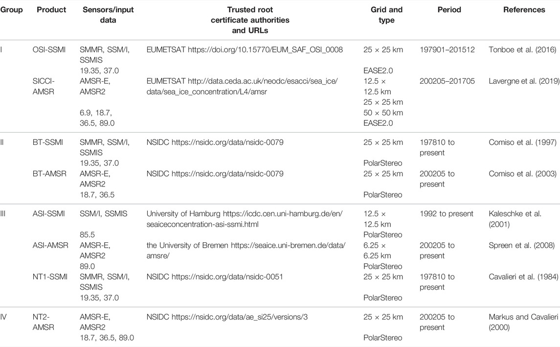
TABLE 2. Overview of passive microwave sea ice concentration retrieval algorithms and products used in this paper (Kern et al., 2019; Kern et al., 2020).
As shown in Table 2, two products, OSI-SSMI and SICCI-AMSR, adopted EASE2.0 projection (equal area grid projection), whereas the other six products adopted polar-stereographic projection. Therefore, the products of OSI-SSMI and SICCI-AMSR needed to be interpolated into the polar-stereographic projection of 25-km grid resolution. The time range of all products selected in this study was from June 2002 to October 2011 and from July 2012 to December 2015.
The AMSR-E/AMSR2 obtained measurements at six/seven different frequencies from 6.9 to 89 GHz with both horizontal and vertical polarization (as shown in Table 1). Compared with SSM/I and SSMIS, the primary improvement with AMSR-E/AMSR2 was a significant increase in spatial resolution because of its footprint size. With the improved spatial resolution, AMSR-E/AMSR2-based sea ice concentration products can monitor more detailed sea ice distributions than those of SSM/I and SSMIS. In this paper, all gridded brightness temperature products of AMSR-E/AMSR2were published by the National Snow and Ice Data Center (NSIDC: https://n5eil01u.ecs.nsidc.org), which provides daily gridded products with 25-km, 12.5-km, and 6.25-km spatial resolution in the polar-stereographic projection. To compare all the sea ice concentration products, the brightness temperature (H or V) products with 25-km spatial resolution in Level 3 were chosen. Brightness temperature of other frequencies was used as a weather filter to remove misestimates of sea ice concentration caused by atmospheric water vapor in some marginal ice zones, at ice edges, and in open water (Markus and Cavalieri, 2000; Comiso et al., 2003; Spreen et al., 2008).
Data on OBS were originally collected by the IceWatch/ASSIST (Arctic Ship-based Sea Ice Standardization) initiative and can be downloaded from http://icewatch.gina.alaska.edu. Kern et al. (2019) processed those data according to the sea ice concentration visual observation methodology recommended by the Antarctic Sea Ice Processes and Climate (ASPeCt) protocol (Worby et al., 2008). Those processed data are available via https://icdc.cen.uni-hamburg.de.html. The ASPeCt protocol was initially proposed for Antarctic sea ice concentration observations and was later enlarged to include Arctic sea ice concentration observations. According to the ASPeCt protocol, the ice condition was observed and recorded every hour (at least every second hour) during daylight when a ship was sailing in ice zones. A standard set of observations was collected from onboard for an area of approximately 1 km around the ship, and the ship’s position, total ice concentration, an estimate of the concentration, thickness, floe size, topography, and snow depth were recorded (Worby and Comiso, 2004).
In this paper, all observations were from June 2002 to December 2019. The distribution of OBS data recorded during this period is shown in Figure 1. Approximately 10,250 individual observations were prepared for this study. Figure 1 shows positions of OBS during the period. Observations were primarily distributed in the Bering Sea, Beaufort Sea, Greenland Sea, and the Central Arctic (north of 80°N), whereas other regions had few or no observations. Grid resolution of the DPR-AMSR was 25 × 25 km, whereas temporal and spatial resolutions of OBS data were much higher than those of DPR-AMSR. Therefore, direct comparison between them was difficult (Worby and Comiso, 2004; Beitsch et al., 2015). To resolve the problem, OBS data and DPR-AMSR data were averaged on each day following the method of Beitsch et al. (2015). Thus, the sea ice concentration of DPR-AMSR was co-located with the OBS by calculating the minimum distance between the OBS location and the grid cell center of DPR-AMSR. In this process, geographic coordinates of all sea ice concentrations were translated to Cartesian coordinates considering the different projections of the sea ice concentration products. Then, daily averages of all ship-based and corresponding satellite-based sea ice concentrations were computed and compared following the approach of Beisch et al. (2015). Data pairs with more than six OBS of sea ice concentration per day were adopted, and 442 days were reserved in this study.
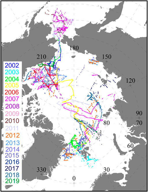
FIGURE 1. Distribution of ship-based observation points in the Arctic region.
Because of the large emissivity differences between water and ice, most sea ice concentration retrieval algorithms employ linear combinations of brightness temperatures (TB) at different frequencies and polarizations to distinguish open water from sea ice (Svendsen et al., 1983; Cavalieri et al., 1984; Spreen et al., 2008; Cho and Naoki, 2015; Lavaergne et al., 2019). Similar to most other sea ice concentration algorithms, the DPR algorithm also uses linear combinations of TB between sea ice and open water. Therefore, TB can be calculated as follows:
where C is the sea ice concentration, Ti is the sea ice temperature, Tw is the seawater temperature, εi is the sea ice microwave emissivity, and εw is the seawater microwave emissivity.
Vertical (V) and horizontal (H) brightness temperatures at the same channel are
Then, solving for those two equations, C can be derived from the following:
where
Scatter plots using dual-polarized brightness temperatures of AMSR2 at 36.5 GHz are shown in Figure 2 for March and September 2013. In the scatter plots, the cluster of data points along the line AD (the slope is 0.92) represents consolidated 100% sea ice (Comiso et al., 2003). Thus, it is expected that the α inferred from Eq. 2a, Eq. 2b would be identical to that from the channel at 36.5 GHz:
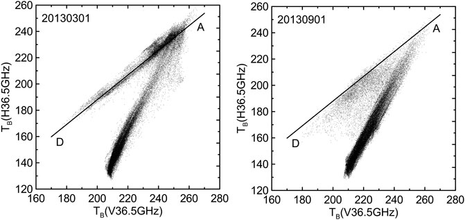
FIGURE 2. Scatter plot of AMSR2 brightness temperature data using H36.5 GHz vs. V36.5 GHz in 2013 on March 1 (left) and September 1 (right). Slope of the line AD is 0.92.
Thus, α is also equal to the slope of the line AD. The DPR algorithm with constant α was used through the whole year and for Arctic to guarantee consistent ice concentration from day to day. The constant
To gain further insight into seasonal and regional stability of α, Zhang et al. (2018) provided a method to automatically ascertain α to reference sea ice concentration. The α adaption was conducted for the 10 years from 2002 to 2011 over the complete Arctic. In this paper, the DPR-AMSR data sets were produced according to the automatic adaptation of α.
The differences in brightness temperatures measured over open water and land can cause spurious sea ice concentration to appear along coasts. There are many methods to reduce this land spill-over effect, which are applied in all sea ice concentration products (Lavergne et al., 2019). For DPR-AMSR, reduction of land spill-over effects is carried out for the ASI-SSMI, ASI-AMSR, NT1-SSMI, and NT2-AMSR. Thus, we do not further correct potential differences by this effect. Meanwhile, the weather filter of DPR-AMSR is similar to ASI-AMSR and NT2-AMSR. These weather filters are based on brightness temperature gradient ratios at 19, 22, and 37 GHz (Cavalieri et al., 1999; Spreen et al., 2008; Zhang et al., 2013).
The products OSI-SSMI and SICCI-AMSR have in common that they are based on a self-tuning, hybrid, self-optimizing sea-ice concentration algorithm (Lavergne et al., 2019). Brightness temperature measured by the SMMR, SSM/I and SSMIS instruments apply this algorithm (Tonboe et al., 2016). Also, it is applied to brightness temperatures observations of the AMSR-E and AMSR2 instruments for the SICCI-AMSR. The two products have not only the same the input satellite data, but also the same processing chains. This algorithm combine three frequency channels (V19 GHz, V37 GHz and H37 GHz). And, they provide best accuracy in Open Water (the
Of which,
The products ASI-SSMI and ASI-AMSR have in common that they are based on ASI algorithm, which is a revised hybrid of the Near 90 GHz algorithm and the NASA Team algorithm (Svendsen et al., 1987; Kaleschke et al., 2001; Spreen et al., 2008). By the brightness temperature polarization difference (P) at ∼90 GHz, water and ice can be distinguished at high resolution.
Based on the Near 90 GHz algorithm, the equation of the ASI algorithm is as followed.
Where, influenced by the atmosphere,
C is the total SIC, T is the temperature,
The ratio of the surface emissivity differences can be assigned a constant value (−1.14). We can use a third order polynomial function to interpolate between the solutions of Eq. 8 to obtain sea-ice concentrations between 0 and 1 as a function of P with the aid of simplification and the assumption that the atmospheric influence inherent in P is a smooth function of the sea-ice concentration.
The coefficients di are derived with a linear equation system based on Eq. 8 and their first derivatives (Spreen et al., 2008).
The products BT-SSMI and BT-AMSR have in common that they are based on BT algorithm (Comiso, 1986; Comiso et al., 1997; Comiso et al., 2003; Comiso and Nishio, 2008), which combines brightness temperature observations in two modes, in frequency mode (37 and 19 GHz, vertical polarization), in polarization mode (37 GHz, vertical and horizontal polarization). It is based on the observation that brightness temperatures measured at these frequencies/polarizations over closed sea ice tend to cluster along a line (ice line) while those tend to cluster around a single point in the respective two-dimensional brightness temperature space over open water. The total sea-ice concentration is calculated as below
The product NT1-SSMI is based on NT1 algorithm (Cavalieri et al., 1984; Cavalieri et al., 1992; Cavalieri et al., 1999), which is a combination of the large difference of the normalized brightness temperature polarization difference at 19 GHz,
In which,
The product NT2-AMSR is based on NT2 algorithm (Markus and Cavalieri, 2000; Comiso and Steffen, 2001; Comiso et al., 2003), which develops to reduce impact such as layering in snow on sea ice on the accuracy of the sea ice concentration obtained with the NT1. The NT2 conceptually differs from the other algorithms presented above. The three relevant parameters (see the equations below) are modelled as a function of SIC in steps of 1% for 12 different atmospheric states using a radiative transfer model. The sea ice concentration is regarded as the retrieved total sea ice concentration, which results in the minimum cost function between modelled and observed values of these parameters. The three relevant parameters used are selected such that the impact of layering in snow on sea ice is mitigated:
In the space, the rotation is given by
Monthly mean sea ice area and sea ice extent derived from DPR-AMSR were compared with those of the other eight sea ice concentration data sets for the entire period. Sea ice extent was calculated as the sum of the total grid-cell area with sea ice concentration >15%, and sea ice area was calculated as the sum of the total ice-covered portion of the grid-cell area with sea ice concentration >15%. There were missing data around the pole because of the satellite orbit inclination and swath width; thus, 100% sea ice concentration was set. Figure 3 shows monthly sea ice area and sea ice extent time series from June 2002 to December 2015 obtained from DPR-AMSR (black curves), as trends for all years (green lines), and as the maximum for March (blue curves) and the minimum for September (red curves). Sea ice area and sea ice extent in the annual trend and for the maximum and the minimum declined significantly. In addition, September trends were much stronger than those in March not only in sea ice area but also in sea ice extent. According to DPR-AMSR, the sea ice area minimum value of 3.02 million km2 and the sea ice extent minimum value of 3.68 million km2 occurred on 15 September 2012.
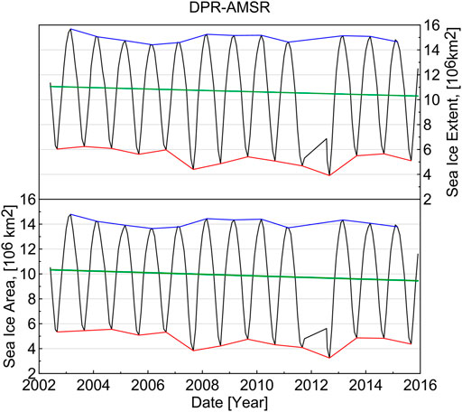
FIGURE 3. Monthly sea ice area and sea ice extent from June 2002 to December 2015 in Arctic obtained from DPR-AMSR. Green lines are trends for all years, blue curves are the maximum for March, and red curves are the minimum for September.
Differences in sea ice area between DPR-AMSR and the other eight sea ice concentration data sets are shown in Figure 4. First, the sea ice area of SICCI-AMSR, OSI-SSMI, and NT1-SSMI are always lower than the DPR-AMSR, with greater differences in summer. Overall mean differences between the DPR-AMSR and SICCI-AMSR, OSI-SSMI, NT1-SSMI were −0.78 ± 0.81 million km2, −0.57 ± 0.59 million km2, and −0.84 ± 0.86 million km2, respectively. In addition, NT1-SSMI provided the smallest sea ice area in summer. Second, the difference in sea ice area between ASI-AMSR (or ASI-SSMI) and DPR-AMSRhas a seasonally variation. The two sea ice concentration estimates were higher than that of DPR-AMSR during summer but were lower during winter, with overall mean differences of −0.16 ± 0.62 million km2 and -0.45 ± 0.67 million km2, respectively. Third, DPR-AMSR results were smaller or larger than those of BT-AMSR, BT-SSMI, and NT2-AMSR. The overall mean differences were −0.10 ± 0.14 million km2, −0.0071 ± 0.093 million km2, and −0.18 ± 0.25 million km2, respectively. Thus, the smallest difference was between BT-SSMI and DPR-AMSR. Results are summarized in Table 3.
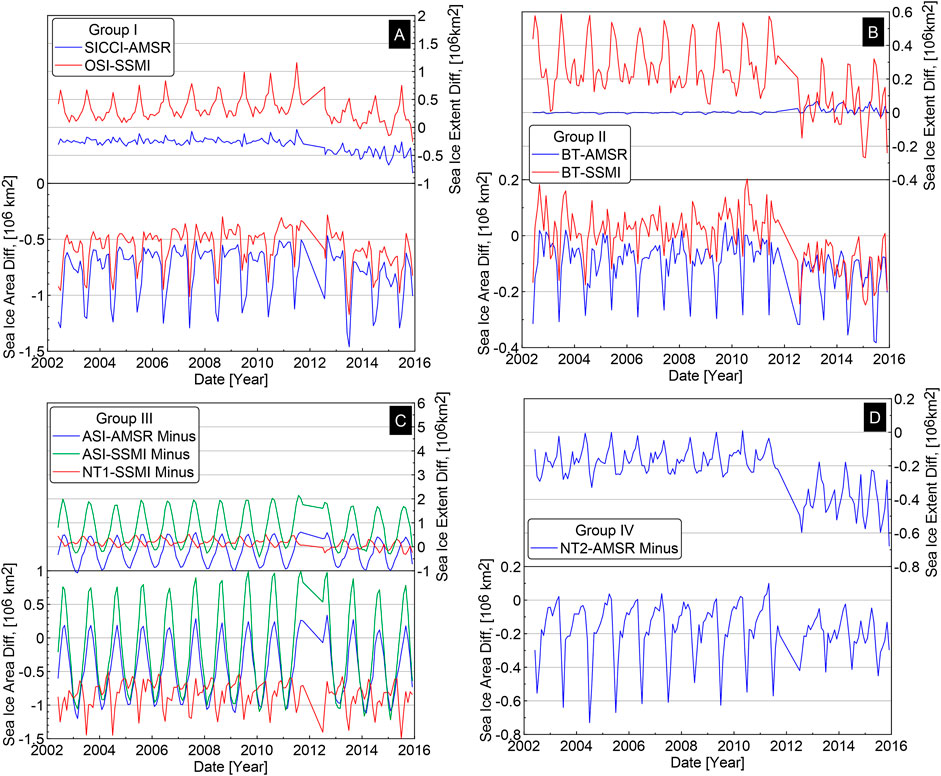
FIGURE 4. Comparison of sea ice area and sea ice extent obtained from eight sea ice concentration data sets with those of DPR-AMSR: (A) include SICCI-AMSR (blue) and OSI-SSMI (red); (B) include BT-AMSR (blue) and BT-SSMI (red); (C) include ASI-AMSR (blue), ASI-SSMI (green) and NT1-SSMI (red); (D) is NT2-AMSR (blue).
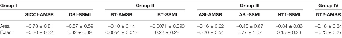
TABLE 3. Overall mean differences in sea ice area and extent. Values are the bias ± root mean square error (unit: 106 km2).
On the one hand, sea ice area is computed by summing over the ice-covered portion of the grid-cell area of grid cells with >15% sea ice concentration. On the other hand, sea ice extent is computed by summing over the grid-cell area of grid cells with >15% sea ice concentration. Thus, the interannual variability of sea ice area and sea ice extent was different between DPR-AMSR and the other eight sea ice concentration data sets (see Figure 4). Sea ice extent of SICCI-AMSR and NT2-AMSR was smaller than that of DPR-AMSR, with differences of −0.30 ± 0.32 million km2 and −0.23 ± 0.27 million km2, respectively. However, sea ice extent of OSI-SSMI and BT-SSMI exceeded that of DPR-AMSR, with differences of 0.32 ± 0.39 million km2 and 0.22 ± 0.28 million km2, respectively. Compared with the sea ice extent of DPR-AMSR, the largest difference was with ASI-SSMI (up to 0.77 ± 1.07 million km2), whereas the smallest difference was with BT-AMSR (only 0.0054 ± 0.017 million km2). Results are also summarized in Table 3.
Two typical monthly mean maps (September and March) of the differences between DPR-AMSR and the other eight sea ice concentration data sets are shown in Figures 5, 7. In the maps, We select the AMSR-E/AMSR2 measurement period (2002–2015) to be able to evaluate and compare DPR-AMSR with the others for a similarly long time-period. The calculations were conducted for the 25-km polar stereographic grid. For comparisons, monthly mean sea ice concentration distribution of DPR-AMSR in September and March is shown in the first subplot of Figures 5, 7, respectively. The corresponding scatterplots between DPR-AMSR and the other data sets are shown in Figures 6, 8, respectively.
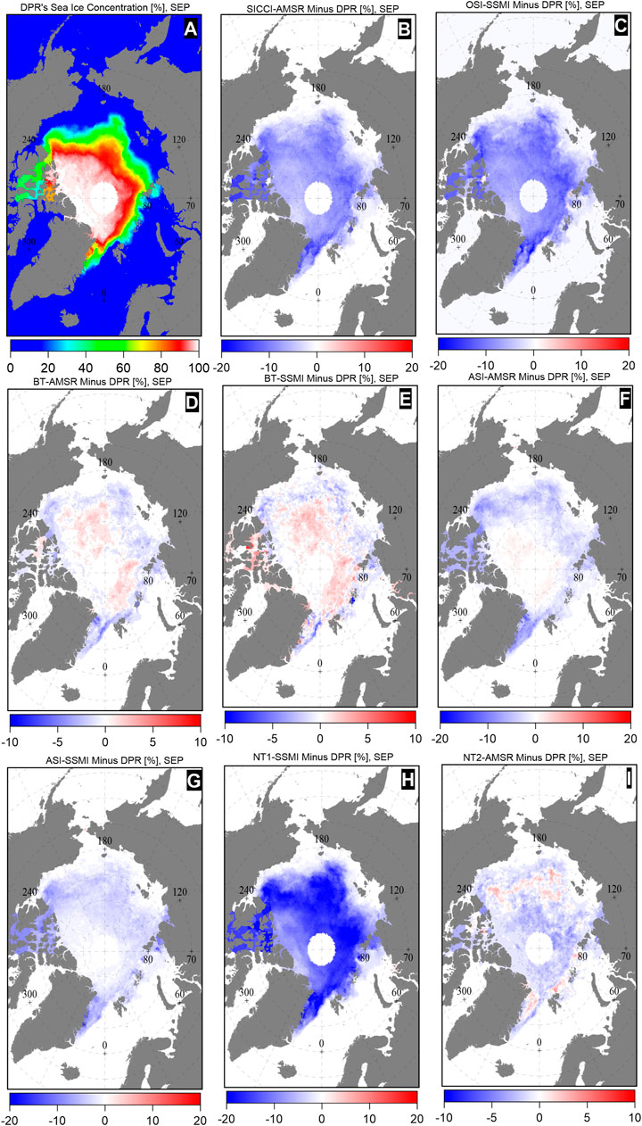
FIGURE 5. Maps of differences between the multi-annual average monthly sea ice concentration of DPR-AMSR and other eight sea ice concentration data sets in September (2002–2015): SICCI-AMSR (B), OSI-SSMI (C), BT-AMSR (D), BT-SSMI (E), ASI-AMSR (F), ASI-SSMI (G), NT1-SSMI (H), and NT2-AMSR (I). (A) is the sea ice concentration map of DPR-AMSR. Differences were only computer for DPR-AMSR sea ice concentration >15%.
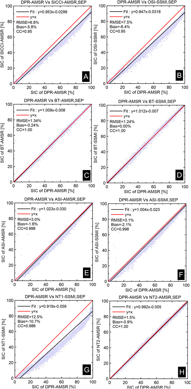
FIGURE 6. Scatterplots of ensemble mean multi-annual average monthly sea ice concentration of DPR-AMSR and other eight sea ice concentration data sets in September (2002–2015): SICCI-AMSR (A), OSI-SSMI (B), BT-AMSR (C), BT-SSMI (D), ASI-AMSR (E), ASI-SSMI (F), NT1-SSMI (G), and NT2-AMSR (H). Red solid lines represent the equality y = x. Black solid lines represent linear fifits of data points. Linear equations, correlation coeffificients (CC), and biases and root mean square errors (RMSE) are also presented.
There were considerable differences between DPR-AMSR and the other eight sea ice concentration data sets in September (Figure 5). Differences in sea ice concentration were particularly negative (DPR-AMSR larger than another sea ice concentration data set) for SICCI-AMSR, OSI-SSMI, ASI-SSMI, and NT1-SSMI. However, differences were in part negative or in part positive (DPR-AMSR smaller than another sea ice concentration data set) for BT-AMSR, BT-SSMI, ASI-AMSR, and NT2-AMSR in pan-Arctic sea ice conditions, with differences of −0.24% ± 1.34%, 0.00% ± 1.24%, −1.6% ± 3.0%, and −0.9% ± 1.5%, respectively (Figure 6). Thus, differences were within ±5% in the overall Arctic Ocean. In addition, BT-SSMI estimated ∼1% more or less sea ice than DPR-AMSR for the sea ice cover regions, whereas ASI-SSIM estimated less sea ice than DPR-AMSR, with differences within −10%–−5% in all MIZs and the Canadian Arctic Archipelago. However, differences in those two sea ice concentration data sets remained within −5%–0.0% over the higher sea ice-covered regions (sea ice concentration >85%), according to Figures 5, 6. The SICCI-AMSR, OSI-SSMI, and NT1-SSMI estimated less sea ice than DPR-AMSR, with differences of −5.8% ± 6.8%, −6.4% ± 7.5%, and −10.7% ± 12.5%, respectively. Moreover, NT1-SSMI produced the lowest overall mean September sea ice concentration, which was lower than that of DPR-AMSR by 15% or even 20% in all sea ice-covered areas.
In March, differences between DPR-AMSR and the eight other sea ice concentration data sets (Figure 7) remained within −5% to 0% over most of the Arctic Ocean, Canadian Arctic Archipelago, and north of Greenland, except for ASI-SSMI, which estimated smaller sea ice concentration with differences less than −5%. The largest differences were distributed in the MIZs and peripheral seas (such as Sea of Okthosk, Bering Sea, Baffin Bay, Greenland Sea, and Barents Sea). The sea ice concentration of BT-AMSR, BT-SSMI, and NT2-AMSR was higher or lower than that of DPR-AMSR but was mostly within ±5%, except around land areas, where sea ice concentration estimates are usually spurious (Lavergne et al., 2019). The distributions of differences for BT-AMSR and BT-SSMI were similar. The overall mean DPR-AMSR in March exceeded SICCI-AMSR, OSI-SSMI, ASI-AMSR, and ASI-SSMI by 5%–15%. Compared with DPR-AMSR, NT1-SSMI underestimated sea ice along the peripheral seas, with differences even less than −15%. For the entire pan-Arctic sea ice (Figure 8), differences between DPR-AMSR and BT-AMSR, BT-SSMI, ASI-AMSR, and NT2-AMSR were −0.53% ± 1.67%, −0.18% ± 2.34%, −1.8% ± 2.9%, and −0.4% ± 1.2%, respectively. Thus, differences were within ±5%. Between DPR-AMSR and SICCI-AMSR, OSI-SSMI, ASI-SSMI, and NT1-SSMI, differences were −3% ± 4%, −2.8% ± 4.3%, −3.9% ± 4.9%, and −3.8% ± 5.9%, respectively. Thus, the differences were mostly less than −5%.
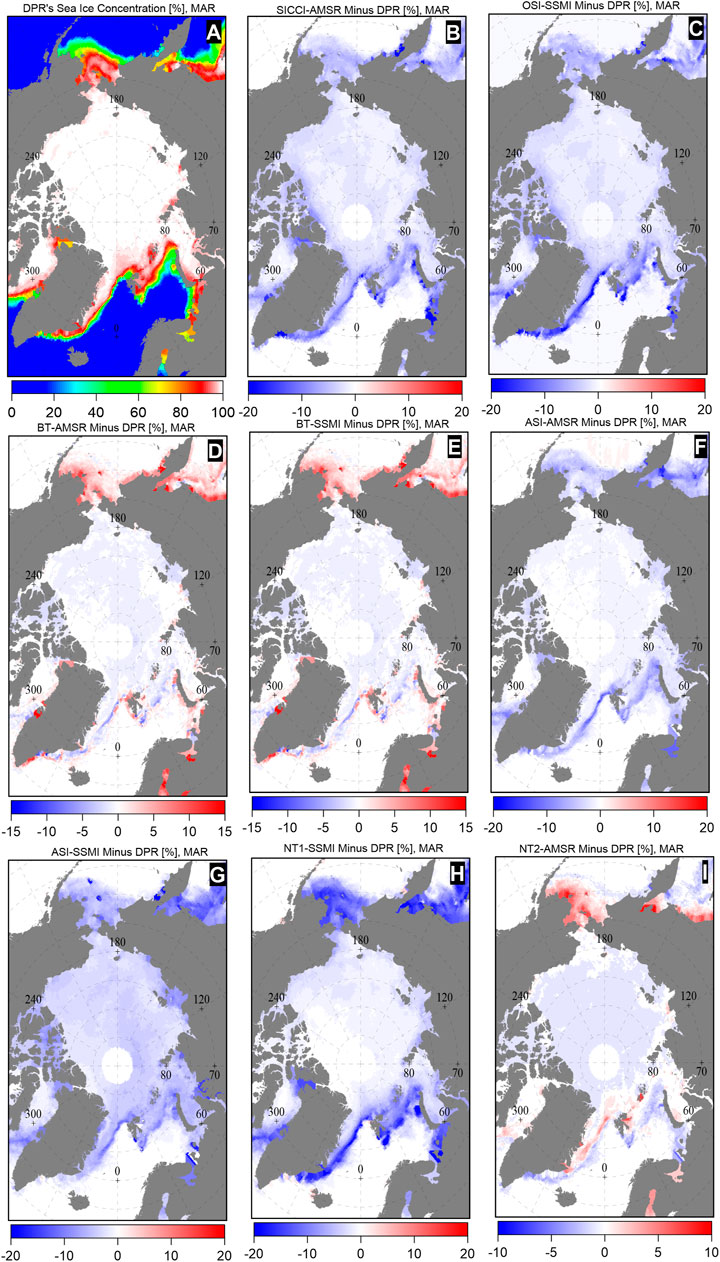
FIGURE 7. Maps of differences between the multi-annual average monthly sea ice concentration of DPR-AMSR and other eight sea ice concentration data sets in March (2002–2015): SICCI-AMSR (B), OSI-SSMI (C), BT-AMSR (D), BT-SSMI (E), ASI-AMSR (F), ASI-SSMI (G), NT1-SSMI (H), and NT2-AMSR (I). (A) is the sea ice concentration map of DPR-AMSR. Differences were only computer for DPR-AMSR sea ice concentration >15%.
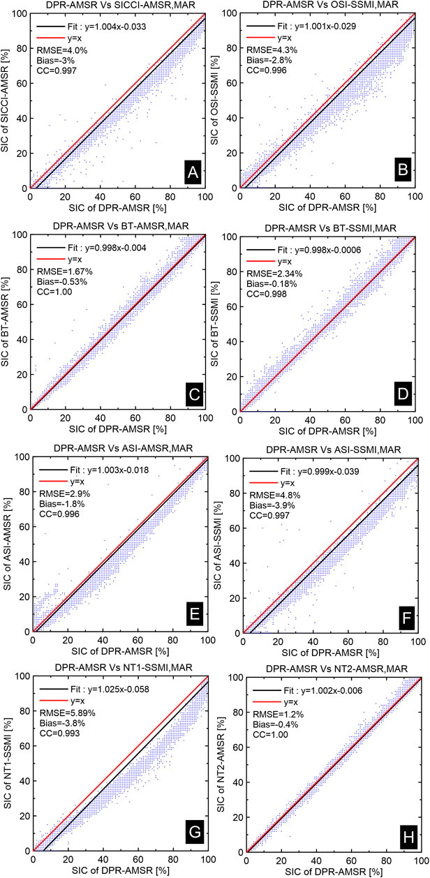
FIGURE 8. Scatterplots of ensemble mean multi-annual average monthly sea ice concentration of DPR-AMSR and other eight sea ice concentration data sets in March (2002–2015): SICCI-AMSR (A), OSI-SSMI (B), BT-AMSR (C), BT-SSMI (D), ASI-AMSR (E), ASI-SSMI (F), NT1-SSMI (G), and NT2-AMSR (H). Red solid lines represent the equality y = x. Black solid lines represent linear fifits of data points. Linear equations, correlation coeffificients (CC), and biases and root mean square errors (RMSE) are also presented.
The histogram in Figure 9 shows the number of sea ice concentration data falling into bins. There were relatively few OBS, less than 50 daily average along-track mean sea ice concentration values for bins <65%. Between 60 and 80 days, OBS fell into bins at 65%–75%, 75%–85%, and >95%. The maximum number of OBS was 107 days for bin 85%–95%. From bin 15%–25% to >95%, days of DPR-AMSR continuously increased from 12 to 160. Days of OBS were fewer than those of DPR-AMSR in bins <15%, 55%–65%, and >95%. In all other bins, there were more OBS days than DPR-AMSR days. Biases and root mean square errors (RMSE) between sea ice concentration of OBS and that of DPR-AMSR are shown in error bars in Figure 10. Bins of 85%–95% and >95% provided the smallest absolute bias of <1%. In the other bins, overall biases were relatively high but did not exceed 10%, except in the 45%–55% bin. The >95% bin had the smallest RMSE of ±5%. The 85%–95% bin had the second smallest RMSE of 13%. The difference between sea ice concentration of OBS and that of DPR-AMSR was less than 15% for sea ice concentration >85%. Thus, the DPR-AMSR was compared reasonably well to the OBS in areas with relatively high sea ice cover.

FIGURE 9. Histogram of co-located daily average sea ice concentrationfrom ship-based visual observations (OBS) (red) and from DPR-AMSR (blue). Data were from 2002 to 2011. sea ice concentrations were separated into the following bins: <15%, 15%–25%, 25%–35%, 35%–45%, 45%–55%, 55%–65%, 65%–75%, 75%–85%, 85%–95%, and >95%.
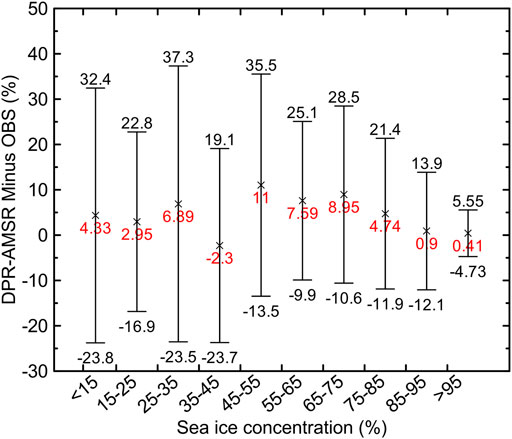
FIGURE 10. Error bars of co-located daily average sea ice concentration from ship-based visual observations (OBS) and from DPR-AMSR. Data were from 2002 to 2011. sea ice concentrations were separated into the following bins: <15%, 15%–25%, 25%–35%, 35%–45%, 45%–55%, 55%–65%, 65%–75%, 75%–85%, 85%–95%, and >95%. Bias (DPR-AMSR sea ice concentration minus OBS) is noted as red numbers.
Figure 11 shows the results obtained for entire years, summers, and winters. Firstly, the two co-located sea ice concentration products were asymmetrically distributed, with sea ice concentration of DPR-AMSR much higher than that of OBS for entire years and summers. Secondly, the two sea ice concentration products were mostly symmetrically distributed around the blue line (y = x). In winter, the difference between sea ice concentration of DPR-AMSR and that of OBS was −3.1% ± 17%, which was somewhat smaller than that in summer (6% ± 18%). Overall, linear correlation coefficients were 0.82, 0.84, and 0.80 for entire years, summers, and winters, respectively. Thus, DPR-AMSR sea ice concentration values were reasonably matched with those of OBS. Additionally, DPR-AMSR data pairs were along the y = 0 sea ice concentration line, which represents that a ship observed sea ice cover but the satellite sensor did’nt. Those data pairs with zero sea ice concentration were very likely the results of the weather filters, which were originally designed to remove the false sea ice caused by atmospheric effects but actually also remove true sea ice (Kern et al., 2019; Xiu et al., 2020).
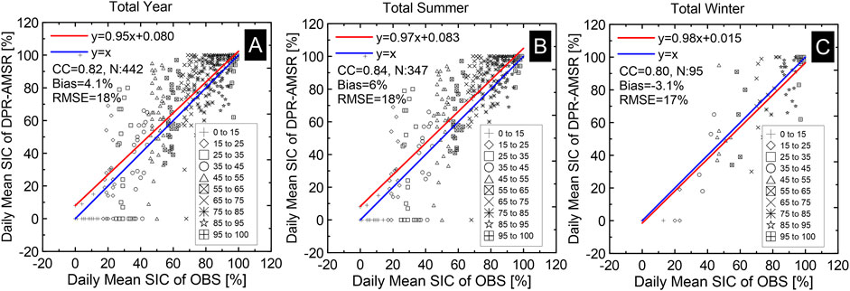
FIGURE 11. Scatterplots of co-located daily average sea ice concentration from ship-based visual observations (OBS) and from DPR-AMSR. Data from 2002 to 2011 were used for (A) years, (B) summers, and (C) winters. Blue solid lines represent the equation y = x. Red solid lines represent linear fits of data points. Linear equations, correlation coefficients (CC), number of valid data pairs (N), and biases and root mean square errors (RMSE) are also presented. Summer includes May, June, July, August, and September; winter includes the other months.
Currently, the channels of AMSR-E/AMSR2 provide higher spatial resolution for extraction of daily available, global sea ice concentration, and BT data than those of SSM/I and SSMIS. The DPR algorithm uses linear combinations of brightness temperatures at dual-polarized 36.5 GHz to retrieve sea ice concentration between 0 and 1. The critical step in the DPR algorithm is how to fix α in Eq. 3. Zhang et al. (2013), Zhang et al. (2018) obtained the value of α via analysis of the respective TB cluster at dual-polarized 36.5 GHz in Figure 2. They noted that the slope of the line AD (the cluster of data pairs along the line AD representing consolidated 100% sea ice) is the value of α. They also fixed dynamic α in time but not in space to reference sea ice concentration (DPR-AMSR), which were compared in this study. The line AD is also used in the Comiso bootstrap algorithm to derive the Arctic sea ice concentration (BT-SSMI and BT-AMSR), but the line is determined in both TB spaces, with TBH37/TBV37 used for sea ice concentration higher than 90% and TBV37/TBV19 used for sea ice concentration lower than 90% (Comiso et al., 1997; Comiso et al., 2003). The SICCI and OSI algorithms also use the line to retrieve sea ice concentration (SICCI-AMSR and OSI-SSMI); however, the line is determined from TB measurements over 100% sea ice within a moving 15-day interval (Kern et al., 2020). All other algorithms of sea ice concentration (NT1-SSMI and NT2-AMSR) are based on the type and update of the tie points of 100% and 0% sea ice concentration. The ASI algorithm uses two fixed tie points (Spreen et al., 2008), and NT1 and NT2 algorithms use fixed tie points for first-year ice and multiyear ice (Markus and Cavalieri, 2009). Thus, in the comparison of all algorithms, the DPR algorithm only needed to determine one parameter from TB spaces, and it provided a more theoretical and simple method to retrieve Arctic sea ice concentration. Furthermore, many attempts demonstrate that Eq. 1 cannot be solved to obtain sea ice concentration because of unknown sea ice microwave emissivity, which depends on sea ice surface temperature, surface roughness, wind, and water vapor (Andersen et al., 2006). However, sea ice concentration can be directly calculated from Eq. 3, which does not use individual sea ice microwave emissivity but uses the ratio of dual-polarized sea ice microwave emissivity. Thus, the DPR algorithm has its unique feature comparing with other algorithms.
Because we don’t know which product provides the best representation of the actual sea ice coverage, one is left with a relatively precise estimate of the sea ice extent, which might likely be biased by an amount an order of magnitude larger. Thus, it is very important to ascertain a standard when we compare DPR-AMSR with other sea ice concentration products. Meier and Steward (2019) pointed out that there was a clear bias (or spread) of 0.5 million km2 to 1.0 million km2 between sea ice extent estimates from different products. Thus, we employed 0.5 million km2 under certain circumstances for the Arctic sea ice extent and sea ice area. At the same time, we employed 5% as a certain circumstances for the difference of sea ice concentration. Currently, DPR-AMSR provides a long-term data set of sea ice concentration, which begins in June 2002. Thus, So it can be used to derive past development or to forecast development of sea ice cover. Meanwhile, all sea ice concentration products in this paper are all popular in climate and ocean studies, and these sea ice concentration products could be well compared with DPR-AMSR.
In sea ice area (Section 4.1), differences were usually less than 0.5 million km2 between DPR-AMSR and BT-AMSR, BT-SSMI, and NT2-AMSR, with BT-SSMI providing the minimum difference (only −0.0071 ± 0.093 million km2) and then ASI-AMSR (0.5–1 million km2). With SICCI-AMSR, OSI-SSMI, ASI-SSMI, and NT1-SSMI, differences often exceeded 1 million km2, with NT1-SSMI providing the maximum difference (−0.84 ± 0.86 million km2). Such differences in sea ice area can often be caused by a difference in sea ice concentration (Section 4.2). Differences were within ±5% between DPR-AMSR and BT-AMSR, BT-SSMI, ASI-AMSR, and NT2-AMSR, with BT-SSMI providing the smallest difference. Differences with ASI-SSIM were within −10% to −5%, whereas differences with SICCI-AMSR, OSI-SSMI, and NT1-SSMI were often less than −10%. NT1-SSMI had the largest difference, which was smaller by 15% or even 20%.
Sea ice extent was calculated from the grid nets of actual sea ice concentration as long as it was above 15%. Thus, interannual differences in sea ice area and sea ice extent were not similar (Section 4.1). With BT-AMSR, BT-SSMI, NT2-AMSR, and NT1-SSMI, differences were relatively small and within 0.5 million km2, with the smallest difference with BT-AMSR of 0.0054 ± 0.017 million km2. With SICCI-AMSR, OSI-SSMI, and ASI-AMSR, the range of differences was 0.5–1 million km2. The largest difference was with ASI-SSMI, which often exceeded 1 million km2 (even up to 2 million km2). According to Kern et al. (2019), such differences in sea ice extent are potentially caused by differences in sea ice concentration in MIZs and along ice edges, in correction of land spillover effect, in a weather filter, or in land-cover fraction.
The DPR algorithm successfully calculated a new operational sea ice concentration for the entire Arctic using AMSR-E/AMSR2 passive microwave brightness temperature (DPR-AMSR). A dynamic parameter (α) was used in the DPR algorithm to retrieve DPR-AMSR. This study focused on comparisons of DPR-AMSR and eight other sea ice concentration products (or OBS) in the Arctic Ocean from June 2002 through December 2015. The primary conclusions are summarized as follow.
First, DPR-AMSR, BT-AMSR, BT-SSMI, and NT2-AMSR provided similar time series of sea ice area and sea ice concentration distribution in the Arctic Ocean. In sea ice area, the absolute difference was usually less than 0.5 million km2, with BT-SSMI with the smallest difference (only −0.0071 ± 0.093 million km2). Differences in sea ice concentration were also within ±5% in the overall Arctic Ocean, and BT-SSMI also provided the smallest difference. However, NT1-SSMI provided the largest difference of sea ice area (−0.84 ± 0.86 million km2) and sea ice concentration distribution, which was lower by 15% or even 20%.
Second, differences in sea ice extent were relatively small and within 0.5 million km2 between DPR-AMSR and BT-AMSR, BT-SSMI, NT2-AMSR, NT1-SSMI. And the smallest difference was with BT-AMSR (0.0054 ± 0.017 million km2). However, The largest difference was with ASI-SSMI, which often exceeded 1 million km2 (even up to 2 million km2 in some seasons).
Third, the comparison of DPR-AMSR with OBS showed that bias and RMSE were relatively small for a high fraction of sea ice concentration in the range 85%–100%. However, bias and RMSE showed an overall increase in other ranges of sea ice concentration. Use of DPR-AMSR resulted in a substantial improvement in the comparison between winter and summer in Arctic, with correlation coefficients increasing and bias and RMSE decreasing.
The results of this study present a process towards a better understanding of the limitations of DPR algorithm, and provide some reference data for improving DPR algorithm. The results of this paper will also help facilitate navigation, climate study and ocean study in the Arctic, especially when only passive microwave data are available. In the future, more systematic and detailed evaluations of DPR-AMSR products in the Arctic will be made on the basis of collecting more in situ observations in various regions and seasons in the Arctic.
The datasets presented in this study can be found in online repositories. The names of the repository/repositories and accession number(s) can be found in the article/Supplementary Material.
SZ and FZ were mainly responsible for the data analysis of all the algorithms; PC, LY, LW, and QS were mainly responsible for downloading and updating the data sets of all the algorithms; JZ gave guidance on the overall conception of the article.
This study was supported by the fundation Variation of Arctic Sea Ice Age and Its Relationship with Atmospheric Circulation Field (PY112101).
The authors declare that the research was conducted in the absence of any commercial or financial relationships that could be construed as a potential conflict of interest.
All claims expressed in this article are solely those of the authors and do not necessarily represent those of their affiliated organizations, or those of the publisher, the editors and the reviewers. Any product that may be evaluated in this article, or claim that may be made by its manufacturer, is not guaranteed or endorsed by the publisher.
We thank the National Snow and Ice Data Center (NSIDC), the University of Bremen, EUMETSAT, and the University of Hamburg for providing the passive microwave sea ice concentration products and OBS products.
Andersen, S., Tonboe, R., Kaleschke, L., Heygster, G., and Pedersen, L. T. (2007). Intercomparison of Passive Microwave Sea Ice Concentration Retrievals over the High-Concentration Arctic Sea Ice. J. Geophys. Res. 112, C08004. doi:10.1029/2006JC003543
Andersen, S., Tonboe, R., Kern, S., and Schyberg, H. (2006). Improved Retrieval of Sea Ice Total Concentration from Spaceborne Passive Microwave Observations Using Numerical Weather Prediction Model fields: an Intercomparison of Nine Algorithms. Remote Sensing Environ. 104 (4), 374–392. doi:10.1016/j.rse.2006.05.013
Beitsch, A., Kern, S., and Kaleschke, L. (2015). Comparison of SSM/I and AMSR-E Sea Ice Concentrations with ASPeCt Ship Observations Around Antarctica. IEEE Trans. Geosci. Remote Sensing 53 (4), 1985–1996. doi:10.1109/TGRS.2014.2351497
Cavalieri, D. J., Crawford, J., Drinkwater, M., Emery, W. J., Eppler, D. T., Farmer, L., et al. (1992). NASA Sea Ice Validation Program for the DMSP SSM/I: Final reportNASA Technical Memorandum 104559. Washington, D.C.: National Aeronautics and Space Administration, 126.
Cavalieri, D. J., Gloersen, P., and Campbell, W. J. (1984). Determination of Sea Ice Parameters with the NIMBUS 7 SMMR. J. Geophys. Res. 89 (D4), 5355–5369. doi:10.1029/jd089id04p05355
Cavalieri, D. J., Parkinson, C. L., Gloersen, P., Comiso, J. C., and Zwally, H. J. (1999). Deriving Long-Term Time Series of Sea Ice Cover from Satellite Passive-Microwave Multisensor Data Sets. J. Geophys. Res. 104 (C7), 15803–15814. doi:10.1029/1999JC900081
Chi, J., Kim, H.-c., Lee, S., and Crawford, M. M. (2019). Deep Learning Based Retrieval Algorithm for Arctic Sea Ice Concentration from AMSR2 Passive Microwave and Modis Optical Data. Remote Sensing Environ. 231, 111204. doi:10.1016/j.rse.2019.05.023
Cho, K., and Naoki, K. (2015). “Advantages of AMSR2 for Monitoring Sea Ice from Space,” in The 36th Asian Conference on Remote Sensing, The Crowne Plaza Manila Galleria in Manila, Philippines, October 19–23, 2015 (Philippines: The Crowne Plaza Manila Galleria in Manila).
Comiso, J. C., Cavalieri, D. J., and Markus, T. (2003). Sea Ice Concentration, Ice Temperature, and Snow Depth Using AMSR-E Data. IEEE Trans. Geosci. Remote Sensing 41 (2), 243–252. doi:10.1109/TGRS.2002.808317
Comiso, J. C., Cavalieri, D. J., Parkinson, C. L., and Gloersen, P. (1997). Passive Microwave Algorithms for Sea Ice Concentration: A Comparison of Two Techniques. Remote Sensing Environ. 60 (3), 357–384. doi:10.1016/S0034-4257(96)00220-9
Comiso, J. C. (1986). Characteristics of Arctic winter Sea Ice from Satellite Multispectral Microwave Observations. J. Geophys. Res. 91 (C1), 975–994. doi:10.1029/JC091iC01p00975
Comiso, J. C. (2009). Enhanced Sea Ice Concentrations and Ice Extents from AMSR-E Data. J. Remote Sensing Soc. Jpn. 29 (1), 199–215. doi:10.11440/rssj.29.199
Comiso, J. C., and Nishio, F. (2008). Trends in the Sea Ice Cover Using Enhanced and Compatible AMSR-E, SSM/I, and SMMR Data. J. Geophys. Res. 113, C02S07. doi:10.1029/2007JC004257
Comiso, J. C., and Steffen, K. (2001). Studies of Antarctic Sea Ice Concentrations from Satellite Data and Their Applications. J. Geophys. Res. 106 (C12), 31361–31385. doi:10.1029/2001JC000823
Gascard, J.-C., Zhang, J., and Rafizadeh, M. (2019). Rapid Decline of Arctic Sea Ice Volume: Causes and Consequences. Cryosphere Discuss., 1–29. doi:10.5194/tc-2019-2
Graham, R. M., Cohen, L., Petty, A. A., Boisvert, L. N., Rinke, A., Hudson, S. R., et al. (2017). Increasing Frequency and Duration of Arctic winter Warming Events. Geophys. Res. Lett. 44 (13), 6974–6983. doi:10.1002/2017gl073395
Ivanova, N., Johannessen, O. M., Pedersen, L. T., and Tonboe, R. T. (2014). Retrieval of Arctic Sea Ice Parameters by Satellite Passive Microwave Sensors: a Comparison of Eleven Sea Ice Concentration Algorithms. IEEE Trans. Geosci. Remote Sensing 52 (11), 7233–7246. doi:10.1109/TGRS.2014.2310136
Ivanova, N., Pedersen, L. T., Tonboe, R. T., Kern, S., Heygster, G., Lavergne, T., et al. (2015). Inter-Comparison and Evaluation of Sea Ice Algorithms: towards Further Identification of Challenges and Optimal Approach Using Passive Microwave Observations. The Cryosphere 9 (5), 1797–1817. doi:10.5194/tc-9-1797-2015
Kaleschke, L., Lüpkes, C., Vihma, T., Haarpaintner, J., Bochert, A., Hartmann, J., et al. (2001). SSM/I Sea Ice Remote Sensing for Mesoscale Ocean-Atmosphere Interaction Analysis. Can. J. Remote Sensing 27 (5), 526–537. doi:10.1080/07038992.2001.10854892
Kern, S., Lavergne, T., Notz, D., Pedersen, L. T., and Tonboe, R. (2020). Satellite Passive Microwave Sea-Ice Concentration Data Set Inter-Comparison for Arctic Summer Conditions. The Cryosphere 14 (7), 2469–2493. doi:10.5194/tc-14-2469-2020
Kern, S., Lavergne, T., Notz, D., Pedersen, L. T., Tonboe, R. T., Saldo, R., et al. (2019). Satellite Passive Microwave Sea-Ice Concentration Data Set Intercomparison: Closed Ice and Ship-Based Observations. The Cryosphere 13 (12), 3261–3307. doi:10.5194/tc-13-3261-2019
Laliberté, F., Howell, S. E. L., and Kushner, P. J. (2016). Regional Variability of a Projected Sea Ice‐Free Arctic during the Summer Months. Geophys. Res. Lett. 43, 256–263. doi:10.1002/2015gl066855
Lavergne, T., Sørensen, A. M., Kern, S., Tonboe, R., Notz, D., Aaboe, S., et al. (2019). Version 2 of the EUMETSAT OSI SAF and ESA CCI Sea-Ice Concentration Climate Data Records. Cryosphere 13 (1), 49–78. doi:10.5194/tc-13-49-2019
Lei, R., Gui, D., Heil, P., Hutchings, J. K., and Ding, M. (2020). Comparisons of Sea Ice Motion and Deformation, and Their Responses to Ice Conditions and Cyclonic Activity in the Western Arctic Ocean between Two Summers. Cold Regions Sci. Technol. 170 (3), 102925. doi:10.1016/j.coldregions.2019.102925
Markus, T., and Cavalieri, D. J. (2000). An Enhancement of the NASA Team Sea Ice Algorithm. IEEE Trans. Geosci. Remote Sensing 38 (3), 1387–1398. doi:10.1109/36.843033
Markus, T., and Cavalieri, D. J. (2009). The AMSR-E NT2 Sea Ice Concentration Algorithm: its Basis and Implementation. J. Remote Sensing Soc. Jpn. 29 (1), 216–225. doi:10.11440/rssj.29.216
Meier, W. N., and Notz, D. (2010). A Note on the Accuracy and Reliability of Satellite-Derived Passive Microwave Estimates of Sea-Ice Extent, Clic Arctic Sea Ice Working Group, Consensus Document. Tromsø, Norway: CLIC International Project Office. 28 October 2010.
Meier, W. N., and Stewart, J. S. (2019). Assessing Uncertainties in Sea Ice Extent Climate Indicators. Environ. Res. Lett. 14 (3), 035005–039326. doi:10.1088/1748-9326/aaf52c
Meredith, M., Sommerkorn, M., Cassotta, S., Derksen, C., Ekaykin, A. A., Hollowed, A., et al. (2019). “Polar Regions,” in IPCC Special Report on the Ocean and Cryosphere in a Changing Climate. Editors H-O. Pörtner, D. C. Roberts, V. Masson-Delmotte, P. Zhai, M. Tignor, E. Poloczanskaet al. In Press.
Pichel, W. G., Clemente-Colón, P., Bertoia, C., Woert, M. V., Wacherman, C. C., Monaldo, F., et al. (2003). “Routine Production of SAR-Derived Ice and Ocean Products in the United States,” in In Proc. 2nd Workshop Coastal and Marine Appl. SAR, Svalbard, Norway, September 8–12, 2003 (ESA Special Publication), 175–182.
Serreze, M. C., Maslanik, J. A., Scambos, T. A., Fetterer, F., Stroeve, J., Knowles, K., et al. (2003). A Record Minimum Arctic Sea Ice Extent and Area in 2002. Geophys. Res. Lett. 30 (3), 1110. doi:10.1029/2002GL016406
Shokr, M., Lambe, A., and Agnew, T. (2008). A New Algorithm (ECICE) to Estimate Ice Concentration from Remote Sensing Observations: An Application to 85-GHz Passive Microwave Data. IEEE Trans. Geosci. Remote Sensing 46 (12), 4104–4121. doi:10.1109/tgrs.2008.2000624
Spreen, G., Kaleschke, L., and Heygster, G. (2008). Sea Ice Remote Sensing Using AMSR-E 89-GHz Channels. J. Geophys. Res. 113 (113), C02S03. doi:10.1029/2005jc003384
Svendsen, E., Kloster, K., Farrelly, B., Johannessen, O. M., Johannessen, J. A., Campbell, W. J., et al. (1983). Norwegian Remote Sensing experiment: Evaluation of the Nimbus 7 Scanning Multichannel Microwave Radiometer for Sea Ice Research. J. Geophys. Res. 88 (C5), 2781–2791. doi:10.1029/JC088iC05p02781
Svendsen, E., Matzler, C., and Grenfell, T. C. (1987). A Model for Retrieving Total Sea Ice Concentration from a Spaceborne Dual-Polarized Passive Microwave Instrument Operating Near 90 GHz. Int. J. Remote Sensing 8 (10), 1479–1487. doi:10.1080/01431168708954790
Tonboe, R. T., Eastwood, S., Lavergne, T., Sørensen, A. M., Rathmann, N., Dybkjær, G., et al. (2016). The EUMETSAT Sea Ice Concentration Climate Data Record. The Cryosphere 10 (5), 2275–2290. doi:10.5194/tc-10-2275-2016
Wayand, N. E., Bitz, C. M., and Blanchard-Wrigglesworth, E. (2019). A Year-Round Subseasonal-To-Seasonal Sea Ice Prediction portal. Geophys. Res. Lett. 46 (6), 3298–3307. doi:10.1029/2018gl081565
Willmes, S., Nicolaus, M., and Haas, C. (2014). The Microwave Emissivity Variability of Snow Covered First-Year Sea Ice from Late winter to Early Summer: a Model Study. The Cryosphere 8 (3), 891–904. doi:10.5194/tc-8-891-2014
Worby, A. P., and Comiso, J. C. (2004). Studies of the Antarctic Sea Ice Edge and Ice Extent from Satellite and Ship Observations. Remote Sensing Environ. 92 (1), 98–111. doi:10.1016/j.rse.2004.05.007
Worby, A. P., Geiger, C. A., Paget, M. J., Woert, V., Ackley, S. F., and Deliberty, T. L. (2008). Thickness Distribution of Antarctic Sea Ice. J. Geophys. Res. Oceans 113 (C05S92), 1–14. doi:10.1029/2007jc004254
Xiu, Y., Li, Z., Lei, R., Wang, Q., Lu, P., and Leppäranta, M. (2020). Comparisons of Passive Microwave Remote Sensing Sea Ice Concentrations with Ship-Based Visual Observations during the CHINARE Arctic Summer Cruises of 2010–2018. Acta Oceanol. Sin. 39 (9), 38–49. doi:10.1007/s13131-020-1646-5
Zhang, S., Zhao, J., Karen, F., and Su, J. (2013). Dual-polarized Ratio Algorithm for Retrieving Arctic Sea Ice Concentration from Passive Microwave Brightness Temperature. J. Oceanography 69 (2), 215–227. doi:10.1007/s10872-012-0167-z
Keywords: Arctic, sea ice concentraiton, brightness temperature, remote sensing products, passive microwave
Citation: Zong F, Zhang S, Chen P, Yang L, Shao Q, Zhao J and Wei L (2022) Evaluation of Sea Ice Concentration Data Using Dual-Polarized Ratio Algorithm in Comparison With Other Satellite Passive Microwave Sea Ice Concentration Data Sets and Ship-Based Visual Observations. Front. Environ. Sci. 10:856289. doi: 10.3389/fenvs.2022.856289
Received: 17 January 2022; Accepted: 04 March 2022;
Published: 04 April 2022.
Edited by:
Lejiang Yu, Polar Research Institute of China, ChinaReviewed by:
Rudiger Gens, University of Alaska Fairbanks, United StatesCopyright © 2022 Zong, Zhang, Chen, Yang, Shao, Zhao and Wei. This is an open-access article distributed under the terms of the Creative Commons Attribution License (CC BY). The use, distribution or reproduction in other forums is permitted, provided the original author(s) and the copyright owner(s) are credited and that the original publication in this journal is cited, in accordance with accepted academic practice. No use, distribution or reproduction is permitted which does not comply with these terms.
*Correspondence: Shugang Zhang, emhhbmdzaHVnYW5nNkAxNjMuY29t
Disclaimer: All claims expressed in this article are solely those of the authors and do not necessarily represent those of their affiliated organizations, or those of the publisher, the editors and the reviewers. Any product that may be evaluated in this article or claim that may be made by its manufacturer is not guaranteed or endorsed by the publisher.
Research integrity at Frontiers
Learn more about the work of our research integrity team to safeguard the quality of each article we publish.