 Chuanxun Yang
 Yangxiaoyue Liu
 Ji Yang5,6
 Shuisen Chen
95% of researchers rate our articles as excellent or good
Learn more about the work of our research integrity team to safeguard the quality of each article we publish.
Find out more
ORIGINAL RESEARCH article
Front. Environ. Sci. , 25 August 2022
Sec. Environmental Informatics and Remote Sensing
Volume 10 - 2022 | https://doi.org/10.3389/fenvs.2022.840540
This article is part of the Research Topic Research of Remote Sensing and Big data Convergence on Environmental Assessments View all 5 articles
The Huang-Huai-Hai River Basin in eastern China has suffered from severe water scarcity during recent decades due to the effects of climate change and human activities. Quantifying the changes in the amount of terrestrial freshwater available in this region and their driving factors is important for understanding hydrological processes and developing a sustainable water policy. This study proposed an ensemble learning model to reconstruct historical variations in the terrestrial water storage (TWS) of the Huang-Huai-Hai River Basin, China. The model was trained using the observations of the variations in TWS from the Gravity Recovery and Climate Experiment mission (GRACE) satellites, climatic driving, and human withdrawal datasets produced on a monthly scale. The variations in the reconstructed TWS were compared with the results of several land surface and hydrological models with a variety of in situ measurements of the soil water content. The contributions of the climate and human activity to the ensemble learning model were also quantified. The results show that the proposed approach generally outperforms the land surface and hydrological models examined in this study, matches the patterns in the GRACE solutions, and reconstructs past changes in TWS, which are consistent with the GRACE observations. Climatic variables are the most important in the ensemble learning model, with precipitation over the prior month being a critical factor. The model that includes human intervention tends to perform better than without it. Irrigation, industry, and domestic water withdrawals contribute equally to the model. This study provides a flexible and easily implementable model that can bridge the gap between GRACE observations and past changes in TWS. The model is applicable in areas with intense human activities, and the results have the potential to be assimilated into and enhance hydrological models.
Monitoring and modeling the dynamics of terrestrial freshwater resources are vital for human beings to cope with the growing global water crisis (Carpenter et al., 2011). Most terrestrial freshwater resources, excluding those in Antarctica and Greenland, are stored as groundwater, which is difficult to sense directly by using conventional satellite-based optical remote sensing (Alsdorf et al., 2007; Wood et al., 2011; Taylor et al., 2012; Gleeson et al., 2015). Although the groundwater table in the wells can be measured, it is difficult to estimate water storage dynamics at the scale of a large basin or continent based on the spatially sparse water table records (Yeh et al., 2006; Voss et al., 2013). Land surface models (LSMs) and global hydrological studies and water resource models (GHWMs) provide alternative ways to understand land water storage and its dynamics on a global basis (Wood et al., 2011; Mo et al., 2016). However, problems can arise, especially over areas in which human activity is intense, as a result of many uncertainties in the experimental parameters, input data and index, and initial conditions of the model (Scanlon et al., 2018). Therefore, the development of alternative methods that can be implemented to monitor and model terrestrial water storage (TWS) is of great significance.
The Gravity Recovery and Climate Experiment (GRACE) satellites, which were launched in 2002, revolutionized the observation and understanding of terrestrial hydro-systems (Rodell, 2004; Yeh et al., 2006; Feng et al., 2013; Save et al., 2016; Scanlon et al., 2016; Wiese et al., 2016; Andrew R. et al., 2017; Scanlon et al., 2018). Compared with global models, GRACE solutions provide a more direct means of measuring variations in global water storage because the satellites measure changes in the Earth’s gravity field by quantifying alterations in the relative distance between the twin GRACE satellites that occur as a result of gravitational changes. After removing noise from the results, such movements can be considered quite relevant to changes in the amount of water stored at a particular place (Save et al., 2016; Sean Swenson, 2006; Watkins et al., 2015). Variations in the TWS that are measured by the GRACE satellites result from the influences of both climatic and human interventions. Therefore, the GRACE solutions provide reliable information about the variation in TWS on a global basis, and the system has been successfully applied in drought mapping (Leblanc et al., 2009), surface water monitoring (Rodell et al., 2009; Huang et al., 2012; Feng et al., 2013), and water balance modeling (Rodell, 2004; Rodell et al., 2011).
Given the higher reliability of this method as compared to LSMs and GHWMs, the results of GRACE total water storage anomalies (TWSA) have the potential for improving models describing TWS dynamics. The assimilation or fusion of the GRACE solutions with land surface models or global reanalysis systems has garnered increasing amounts of attention in recent years (Kumar et al., 2016; Li et al., 2019). The empirical GRACE observations can be integrated using global model outputs by linking TWS-related variables with the TWSA dataset produced by GRACE. Such models can be simplified to linear or polynomial functions that occur between the TWSA and related variables under ideal conditions, and successful experiments have been conducted for the Amazon Basin using this method (Nie et al., 2015; Humphrey et al., 2017). These models are certainly based on a fundamental hypothesis that the mismatches in TWSA and land surface model simulations can be calibrated using typical regression models; however, this assumption is only valid for specific regions and in certain situations. Machine learning is a powerful tool for fitting relations. As reported in previous study (Long et al., 2014), artificial neural networks (ANNs) can produce GRACE TWSA-like predictions for southwestern China that date back to the 1980s by learning the matching patterns between the available GRACE TWSA and independent indicators such as precipitation and soil moisture. Similar experiments were conducted over northwestern China by comparing three machine learning approaches (support vector machine, artificial neural networks, and random forest (RF)) and the general linear regression model (Yang et al., 2018). The empirical results indicated that the RF model outperformed the others and that the linear regression model was not applicable in this area. A recent study has also proven that ensemble learning algorithms perform well when learning the matching patterns between GRACE TWSA and climate forcings (Jing et al., 2020).
However, few experiments have been conducted in areas undergoing intensive irrigation or industrial activity, which are the major human interventions that lead to a decrease in TWS (Feng et al., 2013; Voss et al., 2013). Human withdrawal can be one of the most significant factors that lead to errors in land surface models for heavily irrigated areas (Joodaki et al., 2014; Pokhrel et al., 2017; Tangdamrongsub et al., 2018). In addition, the tools and models that have been initiated for extending the time span covered by GRACE rely heavily on the soil moisture produced by global models or reanalysis systems. This limits the application of the proposed models because they are restricted by the availability of LSMs or the output from reanalysis systems for specific regions and periods. More importantly, it is impossible to separately quantify the contributions of climate and artificial factors with these models due to the dependence on soil moisture variables and the ignorance surrounding human intervention.
This study proposes a machine learning model that can learn the underlying patterns connecting TWS dynamics with variations in the climate and human water withdrawal. The model has been tested in the Huang-Huai-Hai River Basin of China, which is a heavily irrigated area with intensive human activity and is suffering from a water scarcity crisis. A GRACE-consistent TWSA was generated for the study area back to the 1980s and was compared with LSMs/GHWMs and in-situ soil moisture measurements. The significance of the contribution from each factor to the TWSA estimation model is estimated. This study attempts to provide new perspectives for the high-quality modeling of TWS dynamics by using a machine learning framework over areas that suffer from severe human-induced water scarcity. It is highly expected that flexible machine learning tools have great potentials to enrich complex physical models and extend our understanding of TWS modeling for areas such as that studied herein.
The research area covers the Huang-Huai-Hai River Basin in China, which comprises three major river basins: the Yellow River (or Huanghe), Huaihe River, and Haihe River basins. It is located between 95°53′–122°42′E and 30°57′–42°43′N. The areas of the three basins are 752,000 km2 (Yellow River Basin), 274,000 km2 (Huaihe River Basin), and 318,000 km2 (Haihe River Basin). Dominated by low plains and suitable temperatures, the Huang-Huai-Hai River Basin seems abundant as a large block of well cultivated land and is considered one of the most nourished agricultural zones in China. The Huang-Huai-Hai River basin has long been the political and cultural center of China. The cultivated land, population, and gross domestic product (GDP) of this basin account for more than one-third of the national totals, while the amount of water available accounts for approximately 7% of the total (Yan et al., 2013; Yuan et al., 2019). The terrain and climate in the basin changes gradually from west to east; it includes a plateau with a mountain climate, hills with a continental climate, and temperate plains that are affected by monsoon.
The data of terrestrial water storage anomalies (TWSAs) derived from the latest GRACE RL06 Mascon solution produced at the Center for Space Research (CSR), the University of Texas at Austin are used in this study (Save et al., 2016; Save, 2019). The CSR GRACE TWSA dataset is available within the period from January 2003 to June 2017, and the dataset implemented in this study covers the duration from January 2003 to December 2015. The TWSAs produced are relative to the mean baseline for 2004–2009 and are provided on a 1/4 (0.25) degree grid. The gridded TWSA data are rescaled to 1/2 (0.5) degree grids by averaging all the 1/4-degree grids within a 1/2°, which is consistent with the climate data and global model outputs in this study.
The climate data version 4.03 of the Climatic Research Unit Time Series (CRU TS) derived from the University of East Anglia was used as climate forcing data (Harris et al., 2014). The CRU TS dataset was gridded (1/2°) using records from over 4,000 weather sites. Ten variables included in the dataset that have been considered important parameters in the water cycle were used in this study (Table 1).
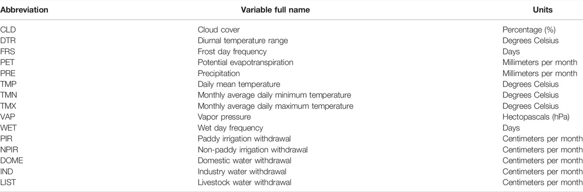
TABLE 1. Variables in the CRU TS climate data.
Water withdrawal data were obtained from the global hydrology model PCR-GLOBWB 2.0, which was developed at Utrecht University (Sutanudjaja et al., 2018). The model uses two sets of computational grids (5 arcmin (1/12 arc-degree) and 30 arcmin (1/2 arc-degree)) that cover 5 continents, excluding Greenland and Antarctica.
Irrigation and non-irrigation water withdrawals were calculated separately in the PCR-GLOBWB 2.0 model. Irrigation water includes paddy water and that used for other agriculture purposes, whereas non-irrigation water covers three sectors: industry, livestock, and domestic water withdrawal. The irrigation water demand is calculated first, and water withdrawal is set to equal the gross water demand unless sufficient water is not available.
The irrigation water demand is calculated from the crop composition (which varies each month and includes multi-cropping) and the area irrigated per cell. The basic dataset is derived from MIRCA 2000, which includes monthly irrigation (paddy and nonpaddy irrigation fractions per cell) and rain-fed crop areas. The total area of irrigation per cell varies over time and is generally based on the area reported by FAOSTAT. The calculation of the amount of water demanded for irrigation follows the FAO guidelines (Rao and Chandran, 1977; Allen et al., 1998; Sutanudjaja et al., 2018). Demand that is not associated with irrigation was calculated using the approaches from (Wada et al., 2014). In cases where available water is insufficient, the water withdrawal amount is measured and scaled down to that of water available and then distributed proportionally to retrieve the gross water demand of every sector.
A dataset comprising 30 arc-minute grid cells from the period 1979–2015 was used in this study. Table 1 summarizes the water withdrawal variables used. Detailed information concerning the PCR-GLOBWB model can be found in (Sutanudjaja et al., 2018).
The auxiliary input data included the digital elevation model (DEM) and data describing the climate zone, which were used to address the complex variations in terrain and climate in the study area. DEM data from the GTOPO30 dataset (https://www.usgs.gov/centers/eros/) were used. The 1/2-degree gridded Köppen-Geiger climate zone data (Kottek et al., 2006) from http://koeppen-geiger.vu-wien.ac.at/were used to describe the climate.
Two global land surface water models and one hydrological research and water resources model are together compared with the TWS reconstructed using the machine learning model. The catchment land surface model (catchment) (Koster et al., 2000) and the Noah model (Chen et al., 1997; Chen et al., 1996; Ek et al., 2003; Koren et al., 1999), which are included in version 2 of the Global Land Data Assimilation (GLDAS-2), are used for comparison, and the datasets are obtained from the website https://disc.gsfc.nasa.gov/datasets. The PCR-GLOBWB model (Sutanudjaja et al., 2018) available at http://www.globalhydrology.nl/is used to describe the hydrology in the study area. It should also be mentioned that the catchment model does not comprise the surface water storage amount and that the groundwater and surface water storage are not simulated by the Noah model, whereas PCR-GLOBWB includes all the TWS components. The PCR-GLOBWB model considers human water consumption, whereas human intervention is not included in the land surface models.
The TWS of the three models is calculated by summing all the available components. The PCR-GLOBWB model is run in a no-human mode (i.e., without human intervention) to assess the impact of human activities factors on the model. The average TWS from 2004 to 2009 is removed from the original TWS to obtain the TWSA before a comparison with the GRACE TWSA. As a result, we refer the TWSA obtained from the catchment, Noah, and PCR-GLOBWB models as catchment TWSA, Noah TWSA, and GLOBWB TWSA, respectively. Additionally, the TWSA of the PCR-GLOBWB model with no artificial intervention is referred to as the GLOBWB(N) TWSA.
The dataset of in-situ cropland soil moisture in China is collected from cropland sites at a temporal resolution of 10 days from 1991 to 2002. The relative soil moisture (unit: %) was provided at five different depths (0–10 cm, 0–20 cm, 0–50 cm, 0–70 cm, and 0–100 cm). The original dataset is obtained from the National Meteorological Information Center of China (http://data.cma.cn/data/). Several of the records from the study period are absent in the original dataset, meaning that preprocessing was required before use. Sites, for which the observation extended over less than 3 years (36 months), were removed; further, because observations were mainly absent at soil depths of 0–70 cm and 0–100 cm, only measurements taken at 0–50 cm were used. The spatial locations of the 29 sites that were selected following pre-processing are shown in Figure 1. The monthly soil moisture data are calculated as the average of the 10-d measurements.
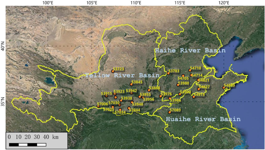
FIGURE 1. Basin boundaries and the locations of in-situ soil moisture sites.
The withdrawal of water produces significant amounts of stress on the water security in northern China, and terrestrial water storage dynamics are under the dual influence of climate change and human activities. The basic concept for the model proposed in this study was to learn the underlying patterns of GRACE TWSA that are associated with climatic and human factors using machine learning algorithms. The validated model was then utilized for the period of 1980s to obtain an extended GRACE-consistent TWSA product. This model considers both climatic and human factors. In addition, the variation in the TWS for a particular basin at a specific time is closely associated with the climate conditions and human activities within the months prior. Thus, the prior conditions were included in the model. The following function gives the expression for the model:
where
The model was designed using two well-known ensemble learning algorithms: random forest (RF) (Breiman, 2001) and extreme gradient boosting (XGB) (Chen and Guestrin, 2016). Ensemble learning algorithms are a type of machine learning mechanism that has been increasingly used for geoscientific applications, showing strong uniqueness and outperforming other machine learning algorithms (Catani et al., 2013; Keller and Evans, 2019; O'Gorman and Dwyer, 2018; Reichstein et al., 2019). The basic concept behind ensemble learning is to combine multiple simple learners to obtain more reliable guides. In addition to their flexibility (no feature normalization is required and simple parameters can be used) and good performance, it is possible to inspect the essence of each variable through variable importance ranking in the RF and XGB models. Successful results have been reported in the evaluation of important variables using the RF algorithm to monitor surface temperature (Hutengs and Vohland, 2016), soil moisture (Long et al., 2019), and groundwater (Rahmati et al., 2016). The random forest (RF) algorithm is widely regarded as one of the best types of ensemble learning algorithms that implements bagging (from bootstrap aggregating). RF uses a bootstrap method that repeatedly draws random subsets from the total training sets with a few replacements. One simple learner (usually a decision tree) is independently generated with each subset (Breiman, 2001), and the final prediction is obtained by averaging the predictions from all the individual trees in the forest.
The XGB model uses the same base learner as the RF model, but a different ensemble strategy is implemented. XGB regression uses a gradient boosting method as an ensemble strategy (Chen and Guestrin, 2016), Gradient boosting is an optimization method that minimizes the residuals by fitting onto the residues forecast by the (i-1)th tree to correct the errors from the predecessors (the ith tree). The performance of the XGB model has not been widely evaluated in earth system modeling, and few studies have compared RF with XGB.
Considering the comparable performance, use of the same base learner, and different ensemble strategies, a comparison of the two ensemble learning models is beneficial for assessing their application in hydrology models. More importantly, because the importance of the variables used in the XGB model can be evaluated using the same approach as RF, interpretation of the variable importance results from the two models is expected to enhance our knowledge of the influence that climate and human factors have on TWS models. Details of the learning process and the variable importance calculation are provided in a previous study (Jing et al., 2020). The models are implemented using Python and the related modules Scikit-learn (Pedregosa et al., 2011) and XGBoost (Chen and Guestrin, 2016).
The evaluation of a model typically relies on cross-validation with randomly sampled subsets. For the ensemble learning models in this study, a cross-validation scheme was used in which the subsets were repeatedly and randomly drawn with replacement for training. Designation is the key point because it improves the stability and accuracy while reducing the likelihood of overfitting. Hence, temporally adjacent years were used for validation in this study instead of cross-validation based on randomly selected subsets.
The validation sets used were temporally adjacent to evaluate the temporal correlations and the capacity of a model to predict a time series for the TWSA. Thus, the period 2003–2015 was divided into two training-validation groups, with the Group 1 (G1) training set covering the period 2006–2015 and validation set covering the period 2003–2005 and the Group 2 (G2) training set describing the period 2003–2011 and validation set covering 2012–2015.
The model was also trained without the inclusion of human factors. The models without human factors are referred to in the following sections (Table 2) as RF(N) and XGB(N), respectively.
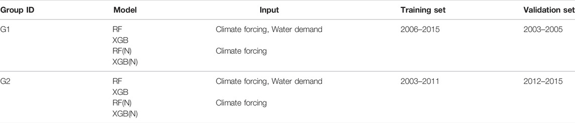
TABLE 2. Arrangement of experimental groups for training and validation.
The validation metrics include the coefficient of determination (R2), correlation coefficient (R), root mean square error (RMSE), and mean error (ME), which are calculated as follows:
In Eq. 2,
There is notable seasonality in the TWSA time series, which has a significant impact on the above error metrics. Therefore, the seasonal cycle needs to be removed from the TWSA time series before the R, ME, and RMSE between the different sources are calculated. Periodic trend decomposition using local regression (STL) is used to remove the periodic cycle. The STL approach proposed by Cleveland et al. (1990). has been increasingly reported as a versatile and moderate method for time-series decomposition (Lu, 2003; Scanlon et al., 2018). The TWSA can be decomposed into three components:
where
where
Figure 2 present the spatial patterns in the estimated TWSA from the RF and XGB models, respectively, for September 2013 which was accompanied by the TWSA form the GRACE CSR-M solution and the global models. The TWSAs produced by the machine learning models (Figures 2B,D) are consistent with the spatial patterns of the TWSAs produced by GRACE. The TWSA without human withdrawal (Figure 2C,E) are less negative than those from the GRACE solutions and the results that include human factors, indicating the significance of human factors in the TWS dynamic model of the basins. The spatial patterns of the TWSA from the global models differ from those produced by GRACE. The TWSA is more negative in catchment than in GRACE for the Huaihe River Basin, while PCR-GLOBWB TWSA is more negative than GRACE in the Haihe River Basin. PCR-GLOBWB without human intervention (PCR-GLOBWB(N)) failed to capture the most negative TWSA grids compared to models including human factors.
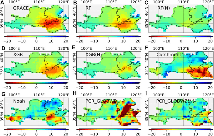
FIGURE 2. Spatial patterns of TWSA for (A) GRACE, (B) RF, (C) RF(N), (D) XGB, (E) XGB(N), (F) Catchment, (G) Noah, (H) PCR-GLOBWB, and (I) PCR-GLOBWB(N) in September 2013 (Unit: cm).
Figure 3 displays the spatial pattern of the RMSE from each model compared with the GRACE solution for the validation set. The LSMs and the PCR-GLOBWB model generally have a higher RMSE compared with GRACE TWSA than the machine learning models, especially in terms of most of the lower Yellow River, Huaihe River, and Haihe River Basins. The inclusion of human withdrawal is beneficial to the machine learning models because a higher RMSE can be seen in the RF(N)/XGB(N) models, especially for G2. The PCR-GLOBWB model with human factors produced a higher RMSE over the Haihe River Basin, the lower stream of Yellow River Basin, and the Hetao Plain than the PCR-GLOBWB(N) model, indicating that the PCR-GLOBWB model overestimated the impact of human withdrawal on the decline in TWS in the Haihe River Basin.
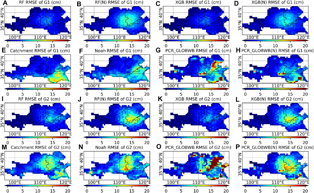
FIGURE 3. Spatial patterns and in the root mean square error (RMSE) of TWSA of GRACE observations and the different models in G1: (A) RF, (B) RF(N), (C) XGB, (D) XGB(N), (E) Catchment, (F) Noah, (G) PCR-GLOBWB, and (H) PCR-GLOBWB(N); and spatial patterns and in the RMSE of TWSA of GRACE observations and the different models in G2: (I) RF, (J) RF(N), (K) XGB, (L) XGB(N), (M) Catchment, (N) Noah, (O) PCR-GLOBWB, and (P) PCR-GLOBWB(N).
Figure 4 together show grid-by-grid scatter plots describing the results of the GRACE TWSA (x-axis) and the TWSA patterns from the machine learning tools and global models (y-axis). Figure 4 displays the validation sets in G1 and G2. According to the results, the machine learning models that included human factors generally outperformed thosethat did not. The RF and XGB models obtained consistent results, and both outperformed the global models examined in this study. Specifically, the R2 values between RF TWSA and GRACE TWSA are 0.64 (G1) and 0.75 (G2), the RMSE is 2.67 cm for G1 and 3.43 cm for G2, and the MEs are all within ±1.0 cm. The results for the XGB TWSA are similar to those of the RF model (Figures 4E,F). The RMSEs of the machine learning model results are close to the claimed uncertainty value of the GRACE CSR-M solution (approximately 2 cm globally), indicating the quality of the results predicted by the machine learning models. The TWSA of the global models, in contrast, demonstrates a lower R2 and a higher RMSE than those from the machine learning models against the GRACE solution.
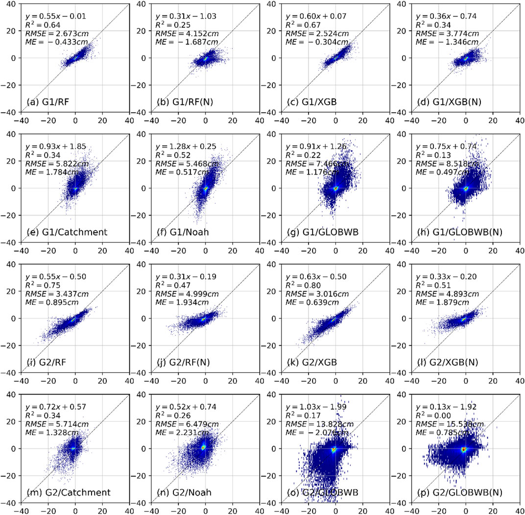
FIGURE 4. Scatter plots between the TWSA of the GRACE observations and different models showing the validation sets for G1: (A) RF, (B) RF(N), (C) XGB, (D) XGB(N), (E) Catchment, (F) Noah, (G) PCR-GLOBWB, and (H) PCR-GLOBWB(N); and scatter plots between the TWSA of the GRACE observations and different models showing the validation sets for G2: (I) RF, (J) RF(N), (K) XGB, (L) XGB(N), (M) Catchment, (N) Noah, (O) PCR-GLOBWB, and (P) PCR-GLOBWB(N).
Although the machine learning models obtained similar R2 values for the two groups in the validation set, the RMSEs in G2 were higher than those in G1. In addition, the discrepancies between the RF/XGB model and the RF(N)/XGB(N) model are more notable in G2 than in G1. The RF/XGB models that include human factors greatly reduce the estimation errors in G2 compared with those that did not include human factors (Figures 4D,H). In G2, the MEs of RF(N) and XGB(N) increase to 1.93 and 1.89 cm, respectively, which are much higher than those produced by the RF and XGB models, suggesting that machine learning models tend to overestimate TWSA values compared to the GRACE solution when human factors are not included and the differences are more evident in G2 than G1.
Figure 5 shows a comparison of the basin-level TWSA time variation series from GRACE, the machine learning models, and the global models considered in this study. The TWSA estimated by the land surface models is more positive than the GRACE TWSA time series. Meanwhile, the TWSA estimated using the machine learning models shows good correlation with the GRACE TWSA time series, while the model without human factors also produces a marginally more positive TWSA than the GRACE solution, especially for G2.
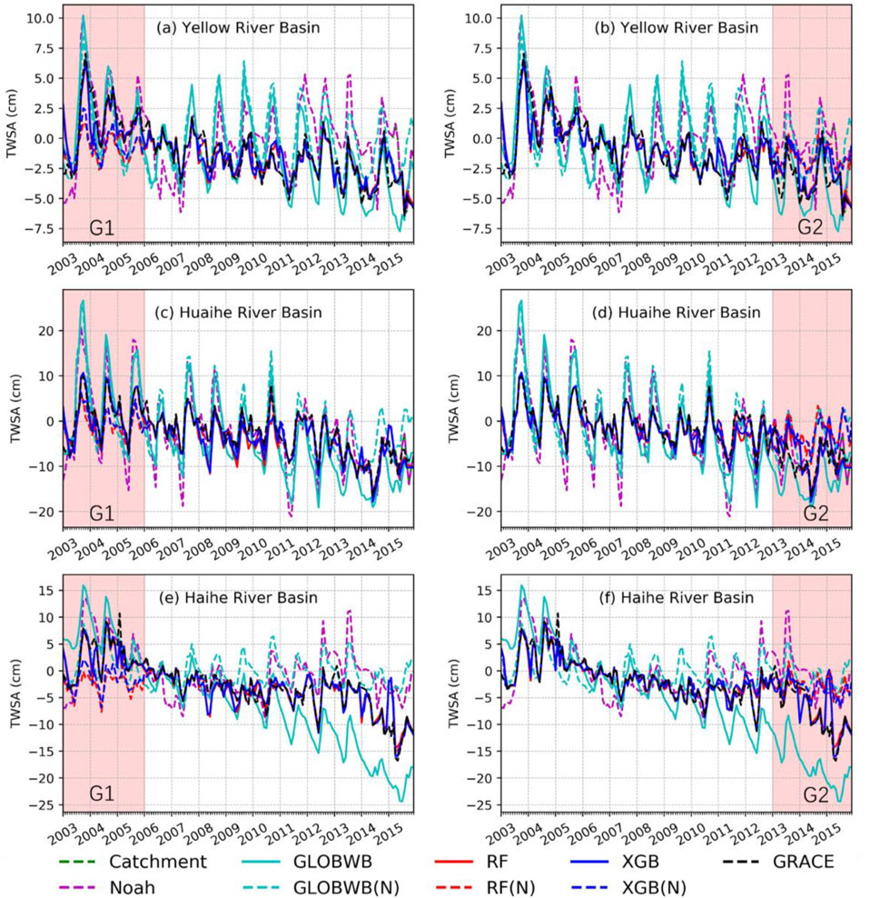
FIGURE 5. Comparison of the Basin level TWSA time series of GRACE observations, different models of the Yellow River Basin in (A) G1, (B) G2, the Huaihe River Basin in (C) G1 and (D) G2, and the Haihe River Basin in (E) G1 and (F) G2 (Red background color indicates the validation period).
According to Figures 5E,F, the PCR-GLOBWB model overestimate the decrease in the TWSA in the Haihe River Basin relative to the GRACE solution. This is consistent with Figures 2H, 4, which implies a more severely negative TWSA of PCR-GLOBWB than that produced by the GRACE solution. Such overestimation of the TWS decline in the Haihe River Basin is partly related to the overestimation of human intervention in the basin because the PCR-GLOBWB(N) model produced more positive and less negative TWSAs for the basin (Figures 5E,F).
Figure 6 present the correlation coefficient (R), RMSE, and ME between the basin-level TWSA from GRACE and the machine learning tools, as well as the globally used models examined in this study. To reduce the influence of seasonal variation, the seasonal components were removed before the values of R, RMSE, and ME were calculated. The RF and XGB TWSA time series for the training set perfectly reproduced the GRACE TWSA time series over the three basins, with a high R (>0.8) and a low RMSE (<2.0 cm). The R for RF/XGB in the G1 validation set was generally higher than that of RF(N)/XGB(N) in the same group. Although similar values of R were obtained for G2 by RF/XGB and RF(N)/XGB(N), the RMSE and ME of the RF(N)/XGB(N) models were much lower than those of RF/XGB. In general, the RF/XGB models outperform RF(N)/XGB(N) with a higher value of R and a lower RSME and ME. Compared with the LSMs and PCR-GLOBWB models, the TWSA estimated using machine learning models is much closer to the GRACE solution, with lower values of RMSE and ME. However, the correlation coefficients of all the machine learning models were lower for the validation set than for the training set. There are two possible reasons for this, the first is that only thirty-six samples (12 months × 3 years) were available for calculating the correlation coefficients of the basin-level TWSA time series in the validation set, and this number of samples may be too small to obtain a valid correlation estimation (Bonett and Wright, 2000); Another reason might be the machine learning models usually perform better in the training set than in the validation set, as the models are trained based on the data in the training set.
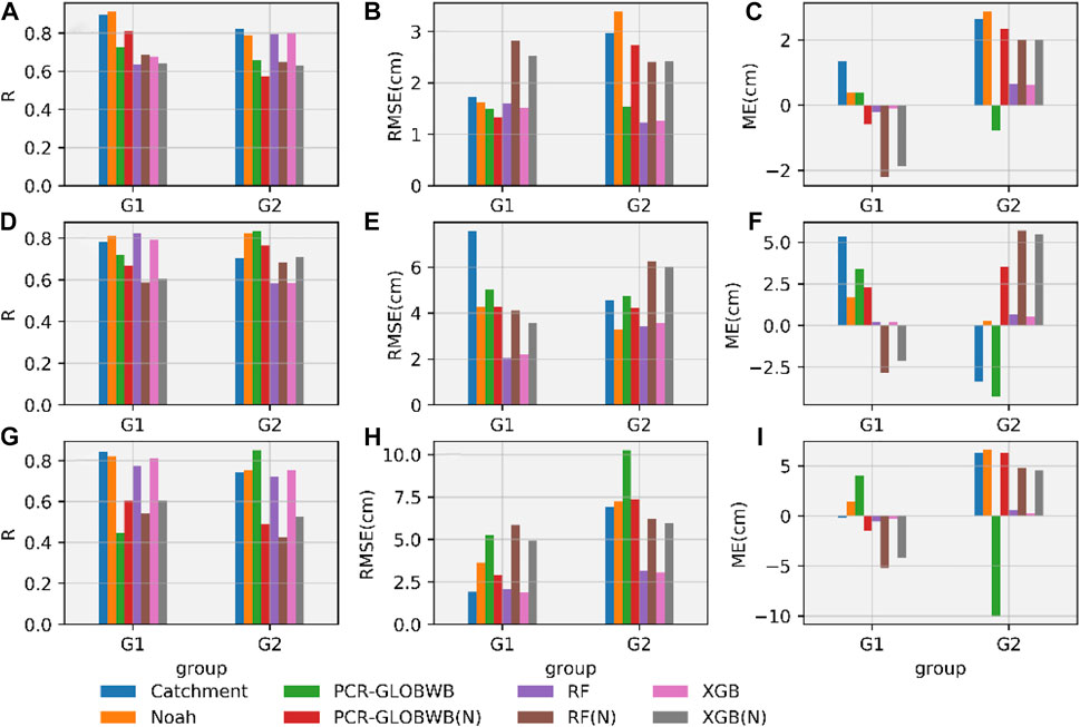
FIGURE 6. (A) Correlation coefficients (R), (B) RMSE, and (C) ME between the de-seasonalized TWSA produced by GRACE observation and the models for the Yellow River Basin from the validation set in G1 and G2; (D) The correlation coefficients (R), (E) RMSE, and (F) ME of the de-seasonalized TWSA of GRACE observation and the unique models for the Huaihe River Basin from validation sets in G1 and G2; (G) The correlation coefficients (R), (H) RMSE, and (I) ME of the de-seasonalized TWSA of GRACE observation and the unique models for the Haihe River Basin from the validation sets in G1 and G2.
The models were trained using datasets covering the entire period of 2003–2015 with human factors and then applied to the period 1979–2015 to generate a value for TWSA that reaches back to 1979. The entire period was divided into three subperiods for analysis: 1979–1990 (P1), 1991–2002 (P2), and 2003–2015 (P3). Figure 7 displays the average TWSA series from the RF and XGB models for the three basins and the TWSA from catchment, Noah, and PCR-GLOBWB. The three subperiods are identified with different panel background colors in the figure. The RF and XGB models produced similar TWSA estimations; therefore, Figure 8 only presents the coefficients of correlation and MEs among the RF TWSA and the three global models after seasonal variations and residuals are removed.
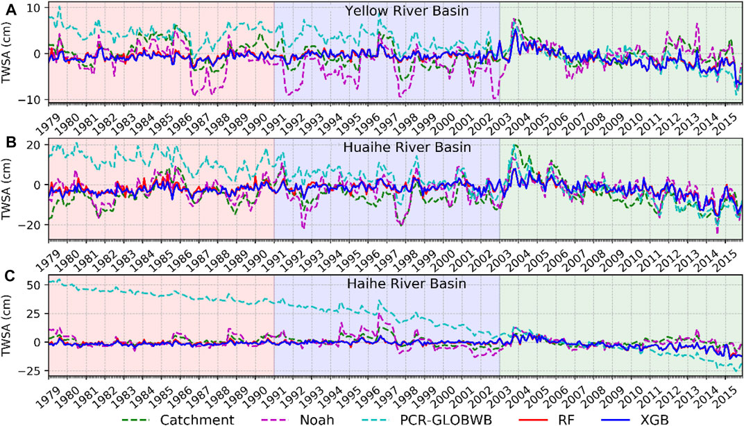
FIGURE 7. Basin level de-seasonalized TWSA time series for the period 1979–2015 from the RF, XGB, Catchment, Noah, and PCR-GLOBWB models in (A) Yellow River Basin, (B) Huaihe River Basin, and (C) Haihe River Basin (P1, P2, and P3 are highlighted by different background colors).
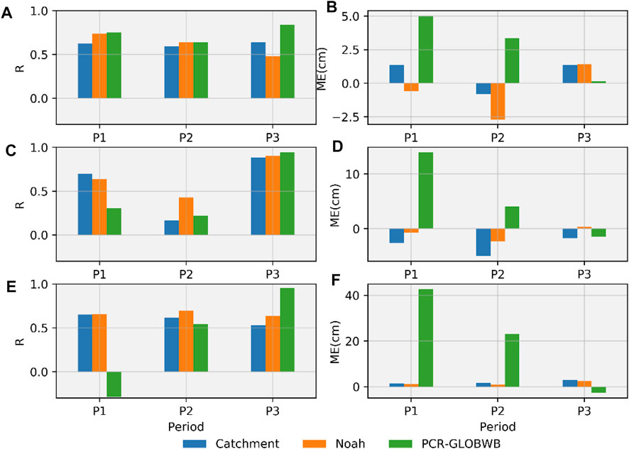
FIGURE 8. (A) Correlation coefficient (R), (B) mean error (ME) between RF TWSA, the TWSA of the Catchment, Noah, and PCR-GLOBWB models over the three sub-periods in the Yellow River Basin; (C) the correlation coefficient (R) and (D) mean error (ME) among he RF TWSA and the TWSA of the Catchment, Noah, and PCR-GLOBWB models for the three sub-periods in Huaihe River Basin; (E) The correlation coefficient (R) and (F) mean error (ME) between the RF TWSA and the TWSA of the Catchment, Noah, and PCR-GLOBWB models for the three sub-periods in Haihe River Basin.
In general, the TWSA reconstructed using machine learning models is well correlated with the TWSA of the LSMs (catchment and Noah) throughout the three subperiods, except for P2 in the Huaihe River Basin (Figure 8A,C,E). The TWSA from the PCR-GLOBWB models shows higher correlation with the reconstructed TWSA but low correlation and high MEs for P1 and P2, especially over the Huaihe and Haihe River Basins (Figure 7). This can also be seen in Figure 8. In addition, the MEs between the RF TWSA and the TWSA from the global model were consistent for the three sub-periods. The measurement errors (RMS of the residuals from STL analysis) of RF and XGB TWSA in the three subperiods were consistent (Table 3). Therefore, the quality of the RF and XGB TWSA for the past few decades is generally stable and in line with the GRACE TWSA for the period 2003–2015.
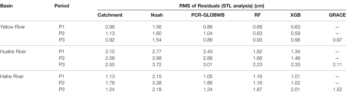
TABLE 3. The root mean square (RMS) of residuals (from STL analysis) for TWSA of different models and GRACE observations during the three sub-periods.
Figure 9 shows a comparison between the RF and XGB TWSAs and the in-situ soil moisture (0–50 cm) at 29 sites in the study area during the period 1991–2002. The correlation coefficients between the two models are shown in Figure 10. Because several of the values for in-situ soil moisture are missing, the number of records available for each site is also shown for reference. According to Figure 10, the variation in the reconstructed TWSA is well correlated with the in-situ soil moisture at most of the sites assessed, and the overall variations in the trends are concurrent. The R value at each site ranged between 0.2 and 0.7, and the average R for all sites was approximately 0.45 (Figures 10B,C). R is lower at all sites without adequate records, such as Nos 53980 and 54705. However, the R value also seems lower than 0.3 at some of the sites with more than 80 records, such as No 53783 and No 57089. The intercorrelations between TWS variations and subsurface water contents have quite a lot to do with the root zone soil moisture and the groundwater levels (Rodell et al., 2009; Tian et al., 2019), and the groundwater amount occupies the majority of the TWS. Although the variations in the sampled soil moisture partially indicate the changes in the regional water storage, the connection between the two parameters looks much weaker than that between groundwater and TWS. In general, the TWSA reconstructed using machine learning tools generally has good agreement with the in situ soil moisture at most of the sites examined in this study. Nevertheless, because a comparison was conducted using soil moisture measurements at 0–50 cm, which only indicates the variations in the water content of the shallow soil layer, the explanation of the results is regarded as indirect rather than validated.
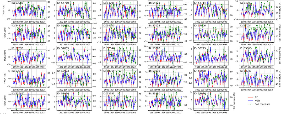
FIGURE 9. The Comparison of TWSA of the RF and XGB models with in-situ soil moisture measurements during the period 1991–2002.
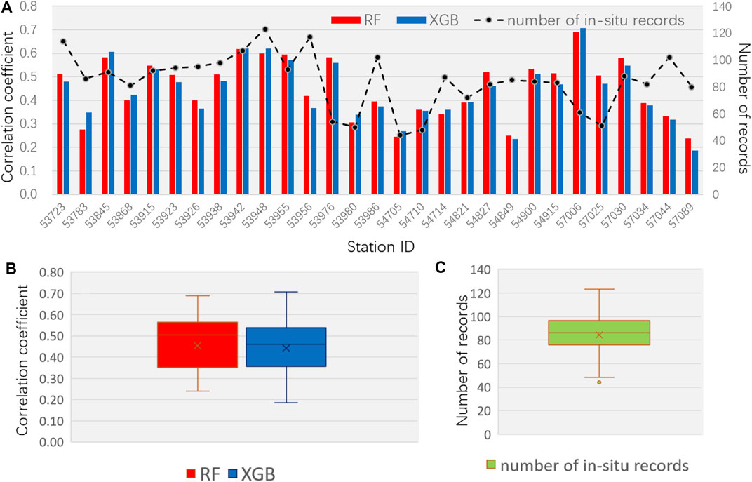
FIGURE 10. (A) Correlation coefficients between RF/XGB TWSA and the in-situ soil moisture on each site, (B) boxplot of the correlation coefficients at all sites, and (C) boxplot showing the of number of records at all sites.
The relative contribution of each variable to the RF and XGB models were also quantified. Figures 11A,B plot the variable importance value (scaled to 0–100) for each variable in the RF and XGB models. The precipitation for the previous one to 3 months (PREt-1, PREt-2, and PREt-3) significantly contributed to the results of both the RF and XGB models. This is in line with the lag in the correlation between variation in the TWS and precipitation. Precipitation takes some time to infiltrate into the root zone soil, after which some of it becomes groundwater, accounting for the majority of the TWS (Sala et al., 1992; Milly, 1994; Andrew R. L. et al., 2017). Thus, the contribution from the precipitation occurring in previous months is rationalized, and the machine learning models effectively learned the close relation between the TWSA and the variation in the precipitation of the study area. The geolocations (LAT and LON) are equally as important as precipitation, suggesting a significant spatial variation in the TWSA of the basin. Latitude is much more important than precipitation in the XGB model.

FIGURE 11. (A) Variable importance values for the RF model at each site, (B) variable significancevalues of the XGB model at each site; summary of variable significance values for the RF model in (C) G1 and (D) G2, and summary of variable significance values for the XGB model in (E) G1 and (F) G2.
Figure 11C–F summarizes the variable importance of the climate forcing, human withdrawal, latitude, longitude, elevation, climate zone, and time variables. In the RF model, the contribution of climate forcing accounts for 66.3–70.8%, and the contribution of the human factor is 17.6–14.4%. The contribution from climate forcing is lower (39.4–50.0%), and the contribution of human factors increases (25.3–21.6%) in the XGB model. Figure 12 illustrates the percentage of each individual variable in terms of climate forcing and human activity. Precipitation dominates the contribution of climate forcing (∼30%) to the models. In the case of human activity, the contribution of nonpaddy irrigation (NPIR) is higher than that of paddy irrigation (PIR) because nonpaddy crops (wheat and maize) are major crops in the Yellow River Basin and Haihe River Basin.
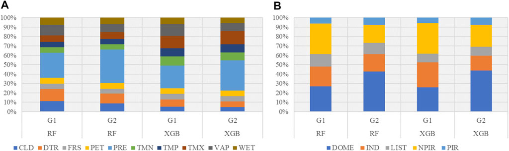
FIGURE 12. (A) Percentage summary of the variable importance of climate variables, and (B) Percentage summary of the variable importance of sectoral water use.
Generally, the contributions of water withdrawals for domestic, industrial, and irrigation use in the models are equal, and the importance value of livestock withdrawal (LIST) is lower than that of the other sectors. Given the dominance of the plains, crop-friendly temperatures, and hours of sunshine, the middle-lower Yellow River basin, Haihe River basin, and Huaihe River basin are considered major bases for the production of grain in China. The irrigation in these areas depends heavily on withdrawal from the groundwater, main rivers, and tributaries (Zheng et al., 2009; Zhao et al., 2014). Coal and iron industries dominate in the middle-lower Yellow River Basin provinces (Ningxia, Shaanxi, and Shanxi provinces) and the Haihe River Basin (Hebei province) (Zhong et al., 2016; Shang et al., 2017). According to Stats, the regional population of the Huang-Huai-Hai River Basin accounts for approximately 35% of the total population of China (Yuan et al., 2019), which gives rise to a huge demand for domestic water. Therefore, the importance contributions of irrigation, industry, and domestic requirements can be expected to be equal, and these patterns were learned well by the machine learning models.
This study proposed a machine learning model for estimating historical variations in the TWS in the Huang-Huai-Hai River Basin. Random forest (RF) and Extreme Gradient Boost (XGB) models were used to train a model that linked GRACE TWSA observations with climate data and human withdrawal. The past GRACE-consistent TWSA was reconstructed by applying this model. The reconstructed TWSA results are compared with the global land surface area and hydrological models, as well as the in situ soil moisture measurements. In addition, the contribution of every variable to the machine learning tool/model was quantified.
In general, the presented approach reproduces spatial patterns and temporal variations in the GRACE TWSA, thereby outperforming a set of global models. The inclusion of human intervention improved the performance of the machine learning model. This is rational because groundwater has been overexploited since the 1970s in the plains of North China, and human activities have profound effects on the changes in the TWS of this region (Kendy et al., 2004; Shi et al., 2011; Cao et al., 2013; Huang et al., 2015; Min et al., 2015). The catchment and Noah models, however, cannot consider human intervention and underestimate the decrease in TWS relative to the GRACE TWSA produced for the research area. These findings are in line with previous research (Mo et al., 2016; Scanlon et al., 2018). The catchment model includes groundwater simulation, enriching the terrestrial water storage components compared with the Noah model. However, the groundwater in the catchment is not directly modeled, and the vertical distribution equilibrium of the soil moisture comprises an implicit water table that is located at the depth of the equilibrium saturation (Kumar et al., 2016). Therefore, there are still many differences between the TWS simulations performed using the catchment model and the GRACE solution.
The PCR-GLOBWB model comprises all the terrestrial water storage models, and because human activities are considered, the TWSA from PCR-GLOBWB presents higher correlations with GRACE TWSA at the basin level. However, the declining trend in the TWS of the Haihe River Basin was overestimated by PCR-GLOBWB relative to the GRACE solution. A similar overestimation of the decline in TWS, which was produced by the PCR-GLOBWB model in this region, was also revealed in another study (Feng et al., 2018). The PCR-GLOBWB model without human intervention underestimated the decrease in the TWS of the Haihe River Basin, indicating that the overestimation of the decline in the TWS by PCR-GLOBWB is a result of the overestimation of human water use in the basin. The machine-learning model used the same calculations that were used for describing water withdrawals in the PCR-GLOBWB model and produced consistent results with the GRACE solution. This indicates that the pattern of climatic and human withdrawals produced by the GRACE TWSA has been successfully calibrated and predicted from the machine learning tool for both the present and past records.
The contribution importance estimations provide an intuitive perspective from which to interpret the ensemble learning models used to estimate TWS changes in this study. Precipitation, acknowledged as the major climatic driving force of variations in the TWS in previous studies (Li et al., 2017; Meng et al., 2019; Xie et al., 2019), is the climatic variable with the highest significance value in the present model. The use of water by three sectors (irrigation, domestic, and industry) has equally important contributions in the model, though not livestock. Some individual variables are more important in the models. In theory, the models consider that only the most important variables would produce comparable results with models that include a full set of variables. For this reason, the RF model is used to select important features describing specific issues (Ham et al., 2005; Chen et al., 2014; Ma et al., 2017). Thus, additional experiments are required in the future to investigate the performance of the models with variables of different sizes.
The variable importance rankings derived from the RF and XGB models are generally similar, except that the human factors and geolocation obtained higher importance values in the XGB model than in the RF model. A possible explanation for this is that the geolocation and human factor contribute more to the residuals of the base learners because the simple learners recursively fit the residuals of their predecessors in the boosting-based ensemble learning model (Freund and Schapire, 1996; Friedman, 2002).
Not every tree in the RF and XGB models includes all the characteristics or observations, which guarantees that the trees are decorrelated and therefore less prone to overfitting. However, correlated features will be issued equal or similar importance, which may reduce the significance compared to the same trees built without their correlated counterparts. In addition, it should be mentioned that the significance value is merely a statistical relative score that does not indicate the authentic contribution of a variable to the TWS, although the RF and XGB models are produced by random selection. The reliability of the results in terms of ranking importance relies on the performance of a model and the selection of the variables used. The notable variables used in this study probably do not cover all types of human intervention or the hydrological factors affecting the TWS dynamics within the headwater of the Yellow River, the Loess Plateau, and the surrounding areas, such as the Three Rivers Source Region Reserve, the Grain for Green project, reservoir operation, and the contribution from snowmelt in the surrounding areas (Jin et al., 2017; Yi et al., 2017; Deng et al., 2018; Lv et al., 2019; Meng et al., 2019; Xie et al., 2019). Therefore, the variable importance results should be explained with additional caution.
The era of big data and artificial intelligence is accelerating the development of data-driven Earth system science. Many machine learning techniques have provided tools and exciting new opportunities for accurately predicting the evolution of water cycles and expanding our understanding of the Earth system from multisource data. We can learn from the results of this study that machine learning and artificial intelligence have the potential to elucidate much more from data than traditional land surface and hydrology models can. However, respecting nature’s physical law is important for expanding our knowledge of the Earth by using machine learning. Therefore, the following key challenge is to develop a hybrid model for coupling physical process models and machine learning approaches.
Because the model input data is not exactly the same as the ensemble learning model, in addition, the GLDAS model also contains input data from other sources, such as land use, soil type and texture, which can cause uncertainty in the GLDAS model. The biases caused by these uncertainties cannot be quantitatively analyzed and discussed in this paper, and the comparison results of GLDAS land surface models need to be further studied.
In summary, the models proposed in this study address how both climate and human factors impact the dynamics of TWS while performing as well as or better than a set of global models in terms of describing areas with intense human activities. Instead of modifying the physical models, the machine learning model is a more flexible, and less expensive alternative for directly reconstructing past changes in the total TWS. The findings of this study enrich our conceptions of the changes and driving forces in the TWS over the Huang-Huai-Hai River Basin and have great potential to be assimilated into hydrological models to improve TWS simulations in the future.
The original contributions presented in the study are included in the article/Supplementary Material, further inquiries can be directed to the corresponding author.
JY and YL conceived and designed the experiments; JY performed the experiments; SC analyzed the data.
This study was jointly supported by the National Natural Science Foundation of China (41801362, 41976190), the Key Special Project for Introduced Talents Team of Southern Marine Science and Engineering Guangdong Laboratory (Guangzhou) (GML2019ZD0301), Guangdong Innovative and Entrepreneurial Research Team Program (2016ZT06D336), GDAS' Project of Science and Technology Development(2019GDASYL-0301001, 2020GDASYL-20200104003), The Science and Technology Program of Guangdong (2021B1212100006). We also thank the Geographical Science Data Center of The Greater Bay Area for providing the relevant data in this study.
The authors declare that the research was conducted in the absence of any commercial or financial relationships that could be construed as a potential conflict of interest.
All claims expressed in this article are solely those of the authors and do not necessarily represent those of their affiliated organizations, or those of the publisher, the editors and the reviewers. Any product that may be evaluated in this article, or claim that may be made by its manufacturer, is not guaranteed or endorsed by the publisher.
Allen, R. G., Pereira, L. S., Raes, D., and Smith, M. (1998). Crop Evapotranspiration-Guidelines for Computing Crop Water Requirements-FAO Irrigation and Drainage Paper 56. Fao, Rome 300 (9), D05109.
Alsdorf, D. E., Rodríguez, E., and Lettenmaier, D. P. (2007). Measuring Surface Water from Space. Rev. Geophys. 45 (2), 2002–2004. doi:10.1029/2006rg000197
Andrew, R., Guan, H., and Batelaan, O. (2017a). Estimation of GRACE Water Storage Components by Temporal Decomposition. J. Hydrol. 552. doi:10.1016/j.jhydrol.2017.06.016
Andrew, R. L., Guan, H., and Batelaan, O. (2017b). Large-scale Vegetation Responses to Terrestrial Moisture Storage Changes. Hydrol. Earth Syst. Sci. 21 (9), 4469–4478. doi:10.5194/hess-21-4469-2017
Bonett, D. G., and Wright, T. A. (2000). Sample Size Requirements for Estimating pearson, Kendall and spearman Correlations. Psychometrika 65 (1), 23–28. doi:10.1007/bf02294183
Cao, G., Zheng, C., Scanlon, B. R., Liu, J., and Li, W. (2013). Use of Flow Modeling to Assess Sustainability of Groundwater Resources in the North China Plain. Water Resour. Res. 49 (1), 159–175. doi:10.1029/2012wr011899
Carpenter, S. R., Stanley, E. H., and Vander Zanden, M. J. (2011). State of the World's Freshwater Ecosystems: Physical, Chemical, and Biological Changes. Annu. Rev. Environ. Resour. 36 (1), 75–99. doi:10.1146/annurev-environ-021810-094524
Catani, F., Lagomarsino, D., Segoni, S., and Tofani, V. (2013). Landslide Susceptibility Estimation by Random Forests Technique: Sensitivity and Scaling Issues. Nat. Hazards Earth Syst. Sci. 13 (11), 2815–2831. doi:10.5194/nhess-13-2815-2013
Chen, F., Janjić, Z., and Mitchell, K. (1997). Impact of Atmospheric Surface-Layer Parameterizations in the New Land-Surface Scheme of the NCEP Mesoscale Eta Model. Boundary-Layer Meteorology 85 (3), 391–421. doi:10.1023/a:1000531001463
Chen, F., Mitchell, K., Schaake, J., Xue, Y., Pan, H.-L., Koren, V., et al. (1996). Modeling of Land Surface Evaporation by Four Schemes and Comparison with FIFE Observations. J. Geophys. Res. 101 (D3), 7251–7268. doi:10.1029/95jd02165
Chen, T., and Guestrin, C. (2016). “Xgboost: A Scalable Tree Boosting System,” in Proceedings of the 22nd acm sigkdd international conference on knowledge discovery and data mining (San Francisco, CA: ACM), 785–794.
Chen, W., Li, X., Wang, Y., Chen, G., and Liu, S. (2014). Forested Landslide Detection Using LiDAR Data and the Random forest Algorithm: A Case Study of the Three Gorges, China. Remote Sensing Environ. 152, 291–301. doi:10.1016/j.rse.2014.07.004
Cleveland, R. B., Cleveland, W. S., McRae, J. E., and Terpenning, I. (1990). STL: A Seasonal-Trend Decomposition. J. Official Stat. 6 (1), 3–73.
Deng, H., Pepin, N., Liu, Q., and Chen, Y. (2018). Understanding the Spatial Differences in Terrestrial Water Storage Variations in the Tibetan Plateau from 2002 to 2016. Climatic change 151 (3-4), 379–393. doi:10.1007/s10584-018-2325-9
Du, P., Bai, X., Tan, K., Xue, Z., Samat, A., Xia, J., et al. (2020). Advances of Four Machine Learning Methods for Spatial Data Handling: a Review. J. Geovis Spat. Anal. 4, 13. doi:10.1007/s41651-020-00048-5
Ek, M. B. (2003). Implementation of Noah Land Surface Model Advances in the National Centers for Environmental Prediction Operational Mesoscale Eta Model. J. Geophys. Res. Atmospheres 108 (D22). doi:10.1029/2002jd003296
Feng, W., Shum, C., Zhong, M., and Pan, Y. (2018). Groundwater Storage Changes in China from Satellite Gravity: An Overview. Remote Sensing 10 (5), 674. doi:10.3390/rs10050674
Feng, W., Zhong, M., Lemoine, J.-M., Biancale, R., Hsu, H.-T., and Xia, J. (2013). Evaluation of Groundwater Depletion in North China Using the Gravity Recovery and Climate Experiment (GRACE) Data and Ground-Based Measurements. Water Resour. Res. 49 (4), 2110–2118. doi:10.1002/wrcr.20192
Freund, Y., and Schapire, R. E. (1996). Experiments with a New Boosting Algorithm. icml. Citeseer, 148–156.
Friedman, J. H. (2002). Stochastic Gradient Boosting. Comput. Stat. Data Anal. 38 (4), 367–378. doi:10.1016/s0167-9473(01)00065-2
Gleeson, T., Befus, K. M., Jasechko, S., Luijendijk, E., and Cardenas, M. B. (2015). The Global Volume and Distribution of Modern Groundwater. Nat. Geosci 9 (2), 161–167. doi:10.1038/ngeo2590
Ham, J., Yangchi Chen, C., Crawford, M. M., and Ghosh, J. (2005). Investigation of the Random forest Framework for Classification of Hyperspectral Data. IEEE Trans. Geosci. Remote Sensing 43 (3), 492–501. doi:10.1109/tgrs.2004.842481
Harris, I., Jones, P. D., Osborn, T. J., and Lister, D. H. (2014). Updated High-Resolution Grids of Monthly Climatic Observations - the CRU TS3.10 Dataset. Int. J. Climatol. 34 (3), 623–642. doi:10.1002/joc.3711
Huang, J. (2012). Detectability of Groundwater Storage Change within the Great Lakes Water Basin Using GRACE. J. Geophys. Res. Solid Earth 117 (B8), 8876. doi:10.1029/2011jb008876
Huang, Z., Pan, Y., Gong, H., Yeh, P. J. F., Li, X., Zhou, D., et al. (2015). Subregional‐scale Groundwater Depletion Detected by GRACE for Both Shallow and Deep Aquifers in North China Plain. Geophys. Res. Lett. 42 (6), 1791–1799. doi:10.1002/2014gl062498
Humphrey, V., Gudmundsson, L., and Seneviratne, S. I. (2017). A Global Reconstruction of Climate‐driven Subdecadal Water Storage Variability. Geophys. Res. Lett. 44 (5), 2300–2309. doi:10.1002/2017gl072564
Hutengs, C., and Vohland, M. (2016). Downscaling Land Surface Temperatures at Regional Scales with Random forest Regression. Remote Sensing Environ. 178, 127–141. doi:10.1016/j.rse.2016.03.006
Jin, Z., Liang, W., Yang, Y., Zhang, W., Yan, J., Chen, X., et al. (2017). Separating Vegetation Greening and Climate Change Controls on Evapotranspiration Trend over the Loess Plateau. Sci. Rep. 7 (1), 8191. doi:10.1038/s41598-017-08477-x
Jing, W. (2020). Can Terrestrial Water Storage Dynamics Be Estimated from Climate Anomalies? Earth Space Sci. 7, e2019EA000959. doi:10.1029/2019ea000959
Joodaki, G., Wahr, J., and Swenson, S. (2014). Estimating the Human Contribution to Groundwater Depletion in the Middle East, from GRACE Data, Land Surface Models, and Well Observations. Water Resour. Res. 50 (3), 2679–2692. doi:10.1002/2013wr014633
Keller, C. A., and Evans, M. J. (2019). Application of Random forest Regression to the Calculation of Gas-phase Chemistry within the GEOS-Chem Chemistry Model V10. Geosci. Model. Dev. 12 (3), 1209–1225. doi:10.5194/gmd-12-1209-2019
Kendy, E., Zhang, Y., Liu, C., Wang, J., and Steenhuis, T. (2004). Groundwater Recharge from Irrigated Cropland in the North China Plain: Case Study of Luancheng County, Hebei Province, 1949-2000. Hydrol. Process. 18 (12), 2289–2302. doi:10.1002/hyp.5529
Koren, V., Schaake, J., Mitchell, K., Duan, Q.-Y., Chen, F., and Baker, J. M. (1999). A Parameterization of Snowpack and Frozen Ground Intended for NCEP Weather and Climate Models. J. Geophys. Res. 104 (D16), 19569–19585. doi:10.1029/1999jd900232
Koster, R. D., Suarez, M. J., Ducharne, A., Stieglitz, M., and Kumar, P. (2000). A Catchment-Based Approach to Modeling Land Surface Processes in a General Circulation Model: 1. Model Structure. J. Geophys. Res. 105 (D20), 24809–24822. doi:10.1029/2000jd900327
Kottek, M., Grieser, J., Beck, C., Rudolf, B., and Rubel, F. (2006). World Map of the Köppen-Geiger Climate Classification Updated. metz 15 (3), 259–263. doi:10.1127/0941-2948/2006/0130
Kumar, S. V., Zaitchik, B. F., Peters-Lidard, C. D., Rodell, M., Reichle, R., Li, B., et al. (2016). Assimilation of Gridded GRACE Terrestrial Water Storage Estimates in the North American Land Data Assimilation System. J. Hydrometeorology 17 (7), 1951–1972. doi:10.1175/jhm-d-15-0157.1
Leblanc, M. J., Tregoning, P., Ramillien, G., Tweed, S. O., and Fakes, A. (2009). Basin‐scale, Integrated Observations of the Early 21st century Multiyear Drought in Southeast Australia. Water Resour. Res. 45 (4). doi:10.1029/2008wr007333
Li, B., Rodell, M., Kumar, S., Beaudoing, H. K., Getirana, A., Zaitchik, B. F., et al. (2019). Global GRACE Data Assimilation for Groundwater and Drought Monitoring: Advances and Challenges. Water Resour. Res. 55 (9), 7564–7586. doi:10.1029/2018wr024618
Li, H., Zhang, Q., Singh, V. P., Shi, P., and Sun, P. (2017). Hydrological Effects of Cropland and Climatic Changes in Arid and Semi-arid River Basins: A Case Study from the Yellow River Basin, China. J. Hydrol. 549, 547–557. doi:10.1016/j.jhydrol.2017.04.024
Long, D., Bai, L., Yan, L., Zhang, C., Yang, W., Lei, H., et al. (2019). Generation of Spatially Complete and Daily Continuous Surface Soil Moisture of High Spatial Resolution. Remote Sensing Environ. 233, 111364. doi:10.1016/j.rse.2019.111364
Long, D., Shen, Y., Sun, A., Hong, Y., Longuevergne, L., Yang, Y., et al. (2014). Drought and Flood Monitoring for a Large Karst Plateau in Southwest China Using Extended GRACE Data. Remote Sensing Environ. 155, 145–160. doi:10.1016/j.rse.2014.08.006
Lu, H. (2003). Decomposition of Vegetation Cover into Woody and Herbaceous Components Using AVHRR NDVI Time Series. Remote Sensing Environ. 86 (1), 1–18. doi:10.1016/s0034-4257(03)00054-3
Lv, M., Ma, Z., Li, M., and Zheng, Z. (2019). Quantitative Analysis of Terrestrial Water Storage Changes under the Grain for Green Program in the Yellow River Basin. J. Geophys. Res. Atmospheres. doi:10.1029/2018jd029113
Ma, L., Fu, T., Blaschke, T., Li, M., Tiede, D., Zhou, Z., et al. (2017). Evaluation of Feature Selection Methods for Object-Based Land Cover Mapping of Unmanned Aerial Vehicle Imagery Using Random Forest and Support Vector Machine Classifiers. Ijgi 6 (2), 51. doi:10.3390/ijgi6020051
Meng, F., Su, F., Li, Y., and Tong, K. (2019). Changes in Terrestrial Water Storage during 2003-2014 and Possible Causes in Tibetan Plateau. J. Geophys. Res. Atmos. 124 (6), 2909–2931. doi:10.1029/2018jd029552
Milly, P. C. D. (1994). Climate, Soil Water Storage, and the Average Annual Water Balance. Water Resour. Res. 30 (7), 2143–2156. doi:10.1029/94wr00586
Min, L., Shen, Y., and Pei, H. (2015). Estimating Groundwater Recharge Using Deep Vadose Zone Data under Typical Irrigated Cropland in the piedmont Region of the North China Plain. J. Hydrol. 527, 305–315. doi:10.1016/j.jhydrol.2015.04.064
Mo, X., Wu, J. J., Wang, Q., and Zhou, H. (2016). Variations in Water Storage in China over Recent Decades from GRACE Observations and GLDAS. Nat. Hazards Earth Syst. Sci. 16 (2), 469–482. doi:10.5194/nhess-16-469-2016
Nie, N., Zhang, W., Zhang, Z., Guo, H., and Ishwaran, N. (2015). Reconstructed Terrestrial Water Storage Change (ΔTWS) from 1948 to 2012 over the Amazon Basin with the Latest GRACE and GLDAS Products. Water Resour. Manage. 30 (1), 279–294. doi:10.1007/s11269-015-1161-1
O'Gorman, P. A., and Dwyer, J. G. (2018). Using Machine Learning to Parameterize Moist Convection: Potential for Modeling of Climate, Climate Change, and Extreme Events. J. Adv. Model. Earth Syst. 10 (10), 2548–2563. doi:10.1029/2018ms001351
Pedregosa, F. (2011). Scikit-learn: Machine Learning in Python. J. machine Learn. Res. 12 (Oct), 2825–2830. doi:10.1524/auto.2011.0951)
Pokhrel, Y. N., Felfelani, F., Shin, S., Yamada, T. J., and Satoh, Y. (2017). Modeling Large-Scale Human Alteration of Land Surface Hydrology and Climate. Geosci. Lett. 4 (1), 10. doi:10.1186/s40562-017-0076-5
Rahmati, O., Pourghasemi, H. R., and Melesse, A. M. (2016). Application of GIS-Based Data Driven Random forest and Maximum Entropy Models for Groundwater Potential Mapping: A Case Study at Mehran Region, Iran. CATENA 137, 360–372. doi:10.1016/j.catena.2015.10.010
Rao, A., and Chandran, M. S. (1977). Crop Water Requirements. Agrometeorol Data Collect Anal. Manag. 51.
Reichstein, M., Camps-Valls, G., Stevens, B., Jung, M., Denzler, J., and Carvalhais, N. (2019). Deep Learning and Process Understanding for Data-Driven Earth System Science. Nature 566 (7743), 195–204. doi:10.1038/s41586-019-0912-1
Rodell, M. (2004). Basin Scale Estimates of Evapotranspiration Using GRACE and Other Observations. Geophys. Res. Lett. 31 (20), 873. doi:10.1029/2004gl020873
Rodell, M., McWilliams, E. B., Famiglietti, J. S., Beaudoing, H. K., and Nigro, J. (2011). Estimating Evapotranspiration Using an Observation Based Terrestrial Water Budget. Hydrol. Process. 25 (26), 4082–4092. doi:10.1002/hyp.8369
Rodell, M., Velicogna, I., and Famiglietti, J. S. (2009). Satellite-based Estimates of Groundwater Depletion in India. Nature 460 (7258), 999–1002. doi:10.1038/nature08238
Sala, O. E., Lauenroth, W. K., and Parton, W. J. (1992). Long-Term Soil Water Dynamics in the Shortgrass Steppe. Ecology 73 (4), 1175–1181. doi:10.2307/1940667
Save, H., Bettadpur, S., and Tapley, B. D. (2016). High-resolution CSR GRACE RL05 Mascons. J. Geophys. Res. Solid Earth 121 (10), 7547–7569. doi:10.1002/2016jb013007
Save, H. (2019). “CSR GRACE RL06 Mascon Solutions,” in Texas Data Repository Dataverse. Editor H. Save.
Scanlon, B. R., Zhang, Z., Save, H., Sun, A. Y., Müller Schmied, H., van Beek, L. P. H., et al. (2018). Global Models Underestimate Large Decadal Declining and Rising Water Storage Trends Relative to GRACE Satellite Data. Proc. Natl. Acad. Sci. U S A. 115 (6), E1080–E1089. doi:10.1073/pnas.1704665115
Scanlon, B. R. (2016). Global Evaluation of New GRACE Mascon Products for Hydrologic Applications. Water Resour. Res. 52, 19494. doi:10.1002/2016wr019494
Sean Swenson, J. W. (2006). Post-processing Removal of Correlated Errors in GRACE Data. Geophys. Res. Lett. 33 (8), L08402.
Shang, Y., Lu, S., Li, X., Hei, P., Lei, X., Gong, J., et al. (2017). Balancing Development of Major Coal Bases with Available Water Resources in China through 2020. Appl. Energ. 194, 735–750. doi:10.1016/j.apenergy.2016.07.002
Shi, J., Wang, Z., Zhang, Z., Fei, Y., Li, Y., Zhang, F. e., et al. (2011). Assessment of Deep Groundwater Over-exploitation in the North China Plain. Geosci. Front. 2 (4), 593–598. doi:10.1016/j.gsf.2011.07.002
Sutanudjaja, E. H., van Beek, R., Wanders, N., Wada, Y., Bosmans, J. H. C., Drost, N., et al. (2018). PCR-GLOBWB 2: a 5 Arcmin Global Hydrological and Water Resources Model. Geosci. Model. Dev. 11 (6), 2429–2453. doi:10.5194/gmd-11-2429-2018
Tangdamrongsub, N., Han, S.-C., Tian, S., Müller Schmied, H., Sutanudjaja, E. H., Ran, J., et al. (2018). Evaluation of Groundwater Storage Variations Estimated from GRACE Data Assimilation and State-Of-The-Art Land Surface Models in Australia and the North China Plain. Remote Sensing 10 (3), 483. doi:10.3390/rs10030483
Taylor, R. G. (2012). Ground Water and Climate Change. Nat. Clim. Change 3, 322. doi:10.1038/nclimate1744
Tian, S., Renzullo, L. J., van Dijk, A. I. J. M., Tregoning, P., and Walker, J. P. (2019). Global Joint Assimilation of GRACE and SMOS for Improved Estimation of Root-Zone Soil Moisture and Vegetation Response. Hydrol. Earth Syst. Sci. 23 (2), 1067–1081. doi:10.5194/hess-23-1067-2019
Voss, K. A., Famiglietti, J. S., Lo, M., de Linage, C., Rodell, M., and Swenson, S. C. (2013). Groundwater Depletion in the Middle East from GRACE with Implications for Transboundary Water Management in the Tigris-Euphrates-Western Iran Region. Water Resour. Res. 49 (2), 904–914. doi:10.1002/wrcr.20078
Wada, Y., Wisser, D., and Bierkens, M. F. P. (2014). Global Modeling of Withdrawal, Allocation and Consumptive Use of Surface Water and Groundwater Resources. Earth Syst. Dynam. 5 (1), 15–40. doi:10.5194/esd-5-15-2014
Watkins, M. M., Wiese, D. N., Yuan, D.-N., Boening, C., and Landerer, F. W. (2015). Improved Methods for Observing Earth's Time Variable Mass Distribution with GRACE Using Spherical Cap Mascons. J. Geophys. Res. Solid Earth 120 (4), 2648–2671. doi:10.1002/2014jb011547
Wiese, D. N., Landerer, F. W., and Watkins, M. M. (2016). Quantifying and Reducing Leakage Errors in the JPL RL05M GRACE Mascon Solution. Water Resour. Res. 52 (9), 19344. doi:10.1002/2016wr019344
Wood, E. F. (2011). Hyperresolution Global Land Surface Modeling: Meeting a Grand challenge for Monitoring Earth's Terrestrial Water. Water Resour. Res. 47 (5), 10090. doi:10.1029/2010wr010090
Xie, J., Xu, Y.-P., Wang, Y., Gu, H., Wang, F., and Pan, S. (2019). Influences of Climatic Variability and Human Activities on Terrestrial Water Storage Variations across the Yellow River Basin in the Recent Decade. J. Hydrol. 579, 124218. doi:10.1016/j.jhydrol.2019.124218
Yan, D. H., Wu, D., Huang, R., Wang, L. N., and Yang, G. Y. (2013). Drought Evolution Characteristics and Precipitation Intensity Changes during Alternating Dry-Wet Changes in the Huang-Huai-Hai River basin. Hydrol. Earth Syst. Sci. 17 (7), 2859–2871. doi:10.5194/hess-17-2859-2013
Yang, P., Xia, J., Zhan, C., and Wang, T. (2018). Reconstruction of Terrestrial Water Storage Anomalies in Northwest China during 1948-2002 Using GRACE and GLDAS Products. Hydrol. Res. 49 (5), 1594–1607. doi:10.2166/nh.2018.074
Yeh, P. J. F., Swenson, S. C., Famiglietti, J. S., and Rodell, M. (2006). Remote Sensing of Groundwater Storage Changes in Illinois Using the Gravity Recovery and Climate Experiment (GRACE). Water Resour. Res. 42 (12), 5374. doi:10.1029/2006wr005374
Yi, S., Song, C., Wang, Q., Wang, L., Heki, K., and Sun, W. (2017). The Potential of GRACE Gravimetry to Detect the Heavy Rainfall-Induced Impoundment of a Small Reservoir in the Upper Yellow River. Water Resour. Res. 53 (8), 6562–6578. doi:10.1002/2017wr020793
Yuan, Y., Yan, D., Yuan, Z., Yin, J., and Zhao, Z. (2019). Spatial Distribution of Precipitation in Huang-Huai-Hai River Basin between 1961 to 2016, China. Int. J. Environ. Res. Public Health 16 (18), 3404. doi:10.3390/ijerph16183404
Zhao, G., Tian, P., Mu, X., Jiao, J., Wang, F., and Gao, P. (2014). Quantifying the Impact of Climate Variability and Human Activities on Streamflow in the Middle Reaches of the Yellow River Basin, China. J. Hydrol. 519, 387–398. doi:10.1016/j.jhydrol.2014.07.014
Zheng, H. (2009). Responses of Streamflow to Climate and Land Surface Change in the Headwaters of the Yellow River Basin. Water Resour. Res. 45 (7), 6665. doi:10.1029/2007wr006665
Keywords: the Huang-Huai-Hai River Basin, GRACE satellites, ensemble learning, terrestrial water storage, reconstructing the historical variations
Citation: Yang C, Liu Y, Yang J, Li Y and Chen S (2022) Reconstructing the Historical Terrestrial Water Storage Variations in the Huang–Huai–Hai River Basin With Consideration of Water Withdrawals. Front. Environ. Sci. 10:840540. doi: 10.3389/fenvs.2022.840540
Received: 21 December 2021; Accepted: 21 March 2022;
Published: 25 August 2022.
Edited by:
Yichun Xie, Eastern Michigan University, United StatesReviewed by:
Min Feng, University of Maryland, United StatesCopyright © 2022 Yang, Liu, Yang, Li and Chen. This is an open-access article distributed under the terms of the Creative Commons Attribution License (CC BY). The use, distribution or reproduction in other forums is permitted, provided the original author(s) and the copyright owner(s) are credited and that the original publication in this journal is cited, in accordance with accepted academic practice. No use, distribution or reproduction is permitted which does not comply with these terms.
*Correspondence: Shuisen Chen, Y3NzQGdkYXMuYWMuY24=
†These authors have contributed equally to this work
Disclaimer: All claims expressed in this article are solely those of the authors and do not necessarily represent those of their affiliated organizations, or those of the publisher, the editors and the reviewers. Any product that may be evaluated in this article or claim that may be made by its manufacturer is not guaranteed or endorsed by the publisher.
Research integrity at Frontiers
Learn more about the work of our research integrity team to safeguard the quality of each article we publish.