Case Analysis of Turbulence From High-Resolution Sounding Data in Northwest China

This study calculated the Thorpe scale, thickness of turbulent layer, turbulent kinetic energy dissipation rate, and turbulent diffusion coefficient based on the Thorpe method using a set of near-space high-resolution radiosonde data in northwest China, and a case study was conducted to analyze the large-scale turbulent layer in the middle stratosphere. The results showed that the most turbulent layers exist near from the middle and upper troposphere to the tropopause region, accounting for 44.0% of the total turbulence, and the largest Thorpe scale and thickness of turbulent layer also appear in this altitude range. In addition, affected by the large-scale turbulence near the tropopause, the calculated turbulent energy dissipation rate and diffusion coefficient also have maximum values at this altitude, which are 0.003 m²s⁻³ and 6.94 m²s⁻¹, respectively. By analyzing the meteorological elements, it is found that there is an obvious correlation between precipitation and large-scale turbulence in the stratosphere. When the precipitation occurs, the corresponding two sets of radiosondes detected larger-scale turbulence layers in the middle stratosphere.

Key Points

1) In this study, a set of near space high-resolution balloon data were used to explore the characteristics of turbulence.

2) The influence of tropospheric meteorological elements on turbulent activities in the stratosphere is studied from a new perspective.

3) It is found that there is a clear relationship between precipitation and the enhancement of the turbulent layer in the middle stratosphere by the Thorpe method.

Introduction

Fluid motion of the atmosphere can be divided into two basic forms, laminar and turbulent flow (Riveros and Riveros-Rosas, 2010). As an important form of the atmospheric motion, turbulence can lead to a certain random overturn and irregular fluctuation in temperature, air pressure, and humidity of each layer (Fritts et al., 2012; Sharman et al., 2012). In the stratified stable atmosphere, when the wind speed and wind shear increase to a certain degree, the gravity wave (Kelvin-Helmholtz wave) becomes unstable in shear and cannot maintain the stable state before, so it breaks into turbulence of different scales, and the kinetic energy is converted into turbulent energy. In the troposphere, thermal convection caused by uneven surface heating and Kelvin-Helmholtz instability are important sources of turbulence (Fritts and Werne, 2000). Thermal convection, latent heat release, strong wind shears, and other factors produce turbulent layers of different scales, causing the atmospheric elements inside the turbulence to mix in different degrees. And the scale of turbulence can reach ranges from a few kilometers to a few millimeters in thickness. Owing to the high randomness of turbulence, its corresponding parameters also have randomness and uncertainty. How to detect turbulence more accurately is of great significance to better understand the mechanism of turbulence action on matter and energy in the atmosphere as well as the spatial and temporal distribution and variation of turbulence.

The detection of atmospheric turbulence is still a complicated problem at present. The use of turbulence probes on airplanes for in-situ detection is expensive and rare (Cohn, 1995). Doppler radar echo is easier to detect turbulence, but the influence of atmospheric uncertainty needs to be considered (Hooper and Thomas, 1998). The estimation of turbulent kinetic energy dissipation rate (TKE) using radar backscattering power requires detection of atmosphere column as auxiliary data. The spectral broadening method will be interfered by other factors except turbulence, and the measurement accuracy of the above two methods in the troposphere is relatively low, so it is difficult to make accurate and reliable turbulence measurement in free atmosphere (Clayson and Kantha, 2008). Owing to the low resolution of the detection data, it is difficult to observe atmospheric turbulence by conventional methods. Thorpe proposed a simple turbulence calculation method to estimate the scale of ocean turbulence mixing overturn and determine the turbulence mixing layer, which provides a good idea for atmospheric turbulence study using conventional sounding data (Thorpe, 1977). Clayson and Kantha (2008) systematically demonstrated the applicability of Thorpe analysis in the free atmosphere using a large number of observational data, and confirmed the feasibility of the Thorpe method in the atmospheric field. The vertical profile of potential density and potential temperature in laminar flow is a monotonic function of altitude. Under the action of turbulence, there will be a certain degree of overturn. The Thorpe method uses the detected basic elements of the atmosphere to calculate the vertical profile of the potential temperature (or potential density), analyzes the difference between the real profile and the profile after monotony sorting, finds the flipping area of potential temperature (potential density), and then calculates the location of turbulent air mass and various turbulence parameters (Kohma et al., 2019). This method provides a new idea for analyzing atmospheric turbulence using conventional radiosonde data with relatively low vertical resolution in the future (Sun et al., 2016; Bellenger et al., 2017; Zhang et al., 2019; He et al., 2020a).

Calculating the turbulence in the free atmosphere from the observed data is helpful to improve the accuracy of numerical weather prediction and climate models. Turbulence caused by jet stream in the tropopause and breaking internal waves near the tropopause is of potential importance in the exchange of trace gases, such as ozone and greenhouse gases. Atmospheric turbulence also plays an important role from the point of view of air passenger safety and comfort. Owing to the lack of atmospheric data of upper troposphere and stratosphere, it is difficult for us to understand the characteristics of small-scale strongly mixed regions (Wilson, 2004). We know that the atmosphere is a chaotic system, although deterministic, it is very sensitive to the disturbance of some weather phenomena (Jonko et al., 2021). In 2020, the average precipitation in China was 695 mm, 10.3% more than that in the previous year. Correct analysis of the coupling relationship between atmospheric turbulence and precipitation and finding the internal relationship are conducive to the prediction of changes in atmospheric turbulence and motion state. In turn, precipitation can be predicted to a certain extent through changes in atmospheric turbulence. It is of great significance to improve the accuracy of weather forecast and numerical weather model (He et al., 2020b).

In this study, Thorpe analysis was performed using data from a near-space sounding balloon in northwest China, which can reach an altitude of more than 35 km. As the first turbulence detection and analysis in the region, this study will help to understand the turbulence distribution in the region and how it relates to local meteorological elements. The second part introduced the data source, the third part introduced the method of data processing of near-space sounding balloon, the fourth part analyzed and discussed the calculation results in detail, and the fifth part summarized and prospected the whole paper.

Data

New Near-Space Sounding Balloon Data

The data used in this study were nine groups of sounding balloons released in northwest China, with latitude and longitude of 100°E and 41°N, ranging from January 10 to 15, 2018. The maximum detection altitude is 45 km, the minimum detection altitude is 34 km, and the average detection altitude is about 40 km, all of which can detect an altitude of more than 30 km. The nine groups of balloons rose at an average speed of 6 meters per second. Owing to the interference of instrument noise and external factors, the detected data would have slight deviation. In this study, cubic spline interpolation was adopted to fit the data profile to eliminate some abnormal deviation values, and all kinds of data were interpolated to the vertical section of 6-m for the convenience of subsequent observation and calculation. The following table lists the launch times and end altitudes of the nine data.

The area released by the sonde is high altitude, and the initial altitude of the detection data reaches 1.025 km.

ERA5 Reanalysis Data

The ERA5 Reanalysis Dataset is the fifth-generation reanalysis calculated by European Centre for Medium-Range Weather Forecasts (ECMWF) for the global climate and weather over the past 40–70 years. The current dataset dates back to 1950. The role of reanalyzes is now widely used together with other datasets (Hersbach et al., 2020). Reanalysis uses the laws of physics to combine model data with observations from around the world to form a globally complete and consistent data set. The horizontal resolution of the data is 0.25° × 0.25°, and the altitude ranges from 1,000 to 1 hPa (Ko and Chun, 2022), with a total of 37 altitude layers and the time resolution of 1 h. This study mainly uses three data sets of total precipitation, air temperature of 2 m on the ground, and surface pressure from January 13 to 15, 2018 to analyze the meteorological elements on the day of turbulence occurrence.

Methods

Turbulence Calculation

The potential temperature calculated from the elements of the atmosphere detected by radiosonde should be monotonically increasing in theory, but due to atmospheric activities such as small-scale turbulence, the corresponding value at certain altitudes has been reversed and changed. The Thorpe method can easily calculate the scale of potential temperature flip. The measured potential temperature profile is reordered as a monotonous profile, and the potential temperature of some heights before and after sorting has shifted. Suppose that a sample of height $z_n$ moves to the position of height $z_m$ after sorting, and the displacement $D=z_m-z_n$ before and after sorting is the calculated Thorpe displacement. The Thorpe scale $L_T$ of the flipped region is calculated from the root mean square of thorpe displacement in the region. Thorpe scale indicates the rollover scale in the atmospheric turbulence layer, under the premise of stable atmospheric stratification, it is related to Ozmidov scale $L_0={(\epsilon /N^3)}^{1/2}$,which describes turbulence characteristics in stable stratified fluids (Riley and Lindborg, 2008), namely

$\begin{array}{c}{\mathit{L}}_0=\mathit{c}{\mathit{L}}_{\mathit{T}}\end{array}(1)$

In the past study, the measurement of the $L_0$ and $L_T$ has been confirmed by the approximate ratio, and near unity when turbulence is fully developed, thus c can be seen as a constant (Riley and Lindborg, 2008; Kantha and Hocking, 2011). $N^2$ is the buoyancy frequency, according to the measured water vapor profile, the relative humidity threshold method is adopted to judge the saturation degree of water vapor in the region. $N^2$ is divided into $N_d^2$ and $N_s^2$, which are buoyancy frequency under unsaturated water vapor and under saturated water vapor respectively (Dale and Durran, 1982).

$\begin{array}{c}{\mathit{N}}_{\mathit{d}}^2=\frac{\mathit{g}}{\mathit{T}}\left[\left(\frac{\mathbf{\partial } \mathbf{T}}{\mathbf{\partial } \mathbf{Z}}\right)+{\mathbf{\Gamma }}_{\mathit{d}}\right]\end{array}(2)$

$\begin{array}{c}{\mathit{N}}_{\mathit{m}}^2=\frac{\mathit{g}}{\mathit{T}}\left[\left(\frac{\mathbf{\partial } \mathbf{T}}{\mathbf{\partial } \mathbf{Z}}\right)+{\mathbf{\Gamma }}_{\mathit{m}}\right]\left[\mathbf{1}+\frac{{\mathit{L}}_{\mathit{v}}{\mathit{q}}_{\mathit{s}}}{\mathit{rt}}\right]-\frac{\mathit{g}}{\mathbf{1}+{\mathit{q}}_{\mathit{w}}}\left(\frac{\mathit{d}{\mathit{q}}_{\mathit{w}}}{\mathit{dz}}\right)\end{array}(3)$

where ${\text{Γ}}_d$ is the dry adiabatic lapse rate, ${\text{Γ}}_m$ is the wet adiabatic lapse rate, $L_v$ is the latent heat of evaporation, $q_s$ is the saturated mixing ratio, $q_w=q_L+q_s$ , $q_L$ is the mixing ratio of liquid water or ice. ε is the dissipation rate of turbulent kinetic energy. According to the Ozmidov scale equation, the relationship between the turbulent kinetic energy dissipation rate ε, the turbulent diffusion coefficient K, and the Ozmidov scale can be obtained as

$\begin{array}{c}\mathbf{\epsilon }={\mathbf{C}}_{\mathbf{k}}{\mathbf{L}}_{\mathbf{T}}^2{\mathbf{N}}^3\end{array}(4)$

$\begin{array}{c}\mathbf{K}=\mathbf{\beta }{\mathit{L}}_0^2\mathbf{N}\end{array}(5)$

where $C_k=c^2$, the value of $C_k$ varies from 0.0625 to 4.0 after measurement. In this study, the parameters used by Clayson and Kantha (2008) were selected for the calculation, $C_k=0.3$, $\beta =\frac{R_f}{1-R_f}$, where $R_f$ is the flux Richardson number, usually 0.25, so β is 1/3, usually 0.3 (Fukao et al., 1994).

Denoising

It is necessary to pay attention to the influence of noise when using data such as atmospheric temperature and air pressure to calculate the potential temperature, which has an important influence on finding the flipping area of potential temperature. Noise removal is an important step to find the potential temperature flipping caused by turbulence. The temperature and air pressure noise caused by the instrument and the environment are important factors for false potential temperature reversal. A variety of methods have been used to remove noise. Wilson et al. (2010) defined the trend-to-noise ratio (TNR), which is defined as the difference between successive sample values in the atmospheric profile divided by the noise standard deviation σ of the sample values. The equation for TNR is as follows:

$\begin{array}{c}\zeta =\frac{{\mathit{\tau }}_{\mathit{i}+1}-{\mathit{\tau }}_{\mathit{i}-1}}{{\mathit{\sigma }}_{\mathit{i}}}\end{array}(6)$

where ${\tau }_i$ is the sample value at i and ${\sigma }_i$ is the noise standard deviation at i. The sample data are divided into several segments, and fitted on each segment. The residual is obtained by calculating the first-order difference between the sample data and the fitted data, and 1/2 of the variance of the residual is the estimate of the noise variance (It should be noted that the calculated noise includes not only pure noise but also some small disturbances). The noise standard deviation of temperature and pressure can be calculated directly from the instrument-measured values, and the potential temperature noise standard deviation will be calculated by the error transfer equation ${\sigma }_{\theta }={\left(\frac{1000}{P}\right)}^{2/7}{\sigma }_T$ (Wilson et al., 2011). The larger the standard deviation of noise in a particular location, the smaller the ζ value. According to the confidence level of false potential temperature flipping, the threshold value of TNR (usually 1) (Zhou, 2018) is set. The sample value corresponding to ζ lower than this threshold is defined as the region with high noise. Bulk TNR is introduced to explain the local trend-to-noise ratio of stratified atmosphere. Bulk TNR has the advantage of considering the vertical stratification of background atmosphere, which is mostly suitable for potential temperature and potential density (Kantha and Hocking, 2011). The size of Bulk TNR is inversely proportional to the standard deviation of noise in the sample area, and inversely proportional to the vertical resolution. Therefore, for the region where the local trend-to-noise ratio is less than the set threshold, the data in the sample area can be smoothed and undersampled by window m (m is set as 2 in this study (He et al., 2020a)) to improve the value of Bulk TNR and reduce the noise level in this area (Zhang et al., 2019).

Even if the under-sampling is performed to the potential temperature data to calculate the Thorpe scale, there are still a certain number of errors in the results obtained. On this basis, statistical tests are performed on the results. Assuming that the number of samples in the flipping area is n and the standard deviation of noise is σ, the potential temperature flipping threshold is set to ${\Delta }_M\theta$. The threshold is obtained by Monte Carlo simulation based on n and σ, and the confidence interval is set as 95%. The noise threshold ${\text{Δ}}_M^{95}\theta$ simulated by the Monte Carlo method is compared with the noise $\text{Δ}\theta$ calculated by the potential temperature flip. When $\text{Δ}\theta <{\text{Δ}}_M^{95}\theta$, the potential temperature flip caused by the sample area is considered to be the flip caused by noise and removed (Wilson et al., 2010).

Results

In this study, nine sets of radiosonde data released in Gansu, China in January 2018 were studied to observe turbulence characteristics. Quality control was carried out on the measured data of atmospheric elements to remove the wrong data. The potential temperature was calculated by using the data after quality control. The detailed background information of the radiosonde data is shown in Table 1.

TABLE 1

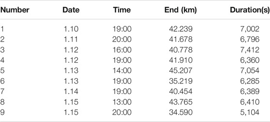
TABLE 1. Basic information of nine deployed sondes, including release Time (Date, Time), End height (End), Duration (Duration).

Figure 1 shows the vertical profile of temperature, air pressure, and potential temperature of nine groups of data. It can be seen from Figure 1A that the stratification between the troposphere and the stratosphere is relatively obvious. The inflection points of the nine sets of temperature profiles are all about at 10 km (which is the lowest point of temperature in the free atmosphere), proving that determined cold points tropopause altitude is about 10 km, which has a relatively good consistency. Figure 1C shows that the calculated potential temperature does not increase monotonously with the altitude and there are a series of disturbances. To pick out potential temperature inversion caused by real turbulence disturbances rather than the noise, the nine sets of potential temperature data are divided into five segments respectively at equal intervals with height, and each segment is used to calculate the Bulk TNR, which is shown in Table 2

FIGURE 1

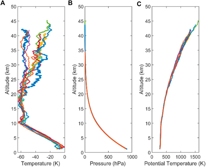
FIGURE 1. Temperature, pressure and potential temperature distribution of 9 sets of radiosonde data. (A–C) show temperature pressure and potential temperature respectively.

TABLE 2

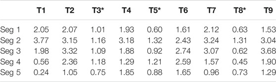
TABLE 2. Bulk TNR distribution of nine sets of data.

Table 2 shows the Bulk TNR distribution of nine sets of data. The T1–T9 of the first line show the nine sets of sounding data, and the Seg 1–Seg 5 of the first column show the five sets of Bulk TNR stratification by height. The T marked with * is the data in the daytime, the others were obtained at night. It can be seen from Table 2 that the Bulk TNR of the low altitude (Seg1–Seg3) is relatively large, and the corresponding altitudes are the troposphere and the lower stratosphere. In this region, there is no large wind shear like the middle and upper stratosphere, the detection height is low, and the noise caused by the instrument is small. The disturbance of each parameter in this region is small and the TNR is higher. In addition, during the day, solar radiation is intense and thermal convection is more obvious, which leads to enhanced air disturbance and enhanced sensitivity of the instrument to noise. Therefore, the Bulk TNR of the three groups of detection data released during the day is smaller than the general one. The segment with Bulk TNR less than 1 was smoothed and undersampled for initial noise removal. The potential temperature profile after reprocessing was calculated by the Thorpe method, and the images of Thorpe scale $L_T$ and Turbulence thickness of the nine sets of sounding data were obtained, which were recorded in Figure 2.

FIGURE 2

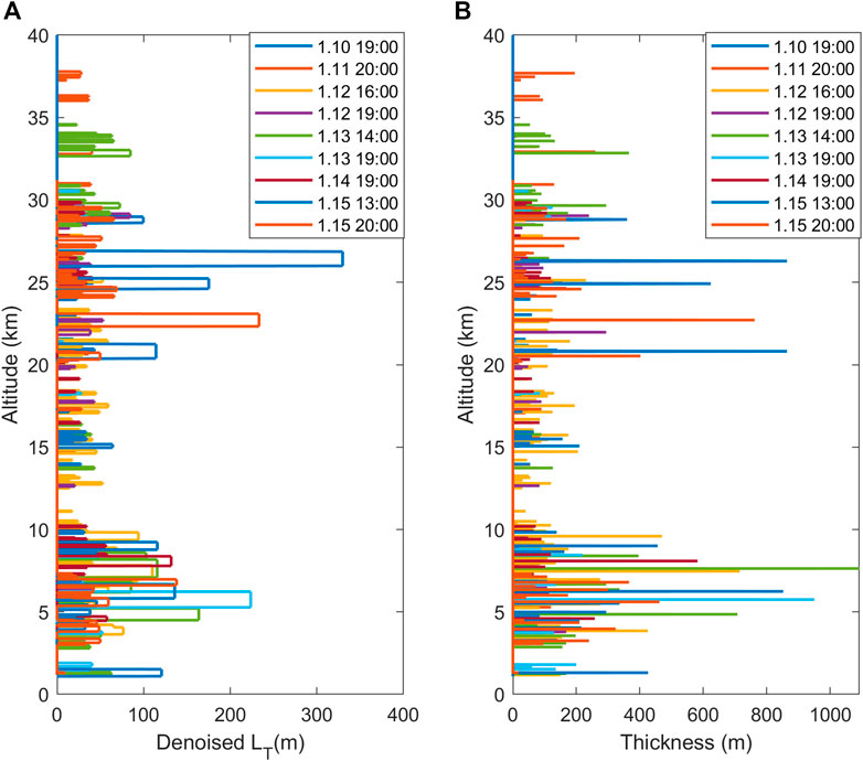
FIGURE 2. Vertical profiles of Thorpe scale and Turbulence thickness of 9 sets of radiosonde data calculated by Thorpe method. (A,B) show Thorpe scale and turbulence thickness respectively.

Figure 2 shows the Thorpe scale and thickness of turbulent layer obtained by the Thorpe method in nine sets of data. As can be seen from Figure 2A, Thorpe scale is concentrated in the middle and upper troposphere, and there are a small number of distributions in the stratosphere, but the scale is small. This is because the troposphere atmosphere disturbance is severe, the atmosphere instability degree is high, the atmosphere changes violently and produces disturbance because of the thermal convection. Figure 2B shows the vertical thickness of potential temperature overturn generated by each turbulence layer, and the turbulence thickness determines the vertical scale of the turbulence layer. It can be seen from Figure 2B that the turbulence thickness generated in the troposphere is generally large, with the maximum value reaching 1,000 m, while the turbulence thickness in the stratosphere is small. Therefore, turbulence intensity in the troposphere is higher than that in the stratosphere, which is consistent with the conclusion given by Wilson et al. (2011). However, it can be seen from Figure 2 that the Thorpe scale and turbulence thickness obtained by calculating the data of the sounding balloon at 13:00 and 20:00 on January 15 showed large values (blue solid line and orange solid line), which is located at 25 km in the lower stratosphere. And the maximum Thorpe scale reaches more than 300 m and turbulence thickness reaches over 500 m (The normal Thorpe scale of the stratosphere is about 50–100 m (Zhang et al., 2019; He et al., 2020a)). Therefore, it is necessary to analyze the atmospheric background and meteorological elements separately to give a reasonable explanation for the occurrence of Thorpe scale outliers in the middle and lower stratosphere on January 15. It can be seen from the above introduction that the meteorological elements that affect the occurrence of turbulence mainly include thermal convection and latent heat release. It is known that the uneven heating of the surface causes gas molecules to rise, and the surrounding gas converges inward to form thermal convection (Chen and Avissar, 1994). Changes in surface temperature will stimulate additional thermal convection (Collow et al., 2014). Surface air pressure is an important factor that characterizes convergence and divergence. Precipitation is the main source of latent heat release, so this study selected surface pressure, the surface air temperature, and precipitation as the weather factors to explore the development of turbulence.

Considering that the sounding balloon does not rise vertically, it will drift with the wind in the horizontal direction during the ascent. This study selected ERA5 reanalysis data from 40°N to 42°N and 100°E to 103.25°E for analysis based on the horizontal trajectory of three groups of sounding balloons, and obtained the following image.

Figure 3 shows the distribution of surface air pressure, surface air temperature, and total precipitation in the range of 100°–103.25° E and 40°–42°N from January 13 to 15. The temperature data vary greatly from day to night. Considering that the release time of sounding balloon on January 15 is 13:00 and 20:00, therefore, the temperature data are only calculated as the average of 12 sets of data between 08:00 and 20:00 of the day. In the figure, the release position of the sounding balloon is represented by the red circle, and the black solid point is the horizontal flight track of the sounding balloon on that day. It can be seen from Figures 3A–C that the surface pressure did not change significantly from January 13 to 15. The surface pressure of the three figures showed a trend of low in southeast and high in northwest, and the horizontal trajectory of the balloon flight was roughly the same, drifting to the east and lifting slightly to the north. There was no pressure disturbance on the drifting path. The air temperature shown in Figures 3D–F was higher in the southwest and lower in the northeast. In the observed area, the temperature rose by about 2K on January 14. However, the surface atmospheric temperature on January 13 and 15 was roughly the same, so it was not considered as the cause of increasing turbulence. It can be seen from Figures 3G–I that there was a small amount of precipitation in the flight area of the sounding balloon on January 15, and a small amount of precipitation occurred in the northeast of the sounding area on January 14, but the precipitation intensity was small and did not cover the flight track of the balloon. There was no precipitation on January 13. Therefore, it is considered that there is a certain relationship between the two groups of large-scale stratospheric turbulence measured on January 15 and the precipitation in this region. Further analysis was made on the precipitation distribution, and the 4-h distribution of precipitation on January 15 was observed, as shown in Figure 4

FIGURE 3

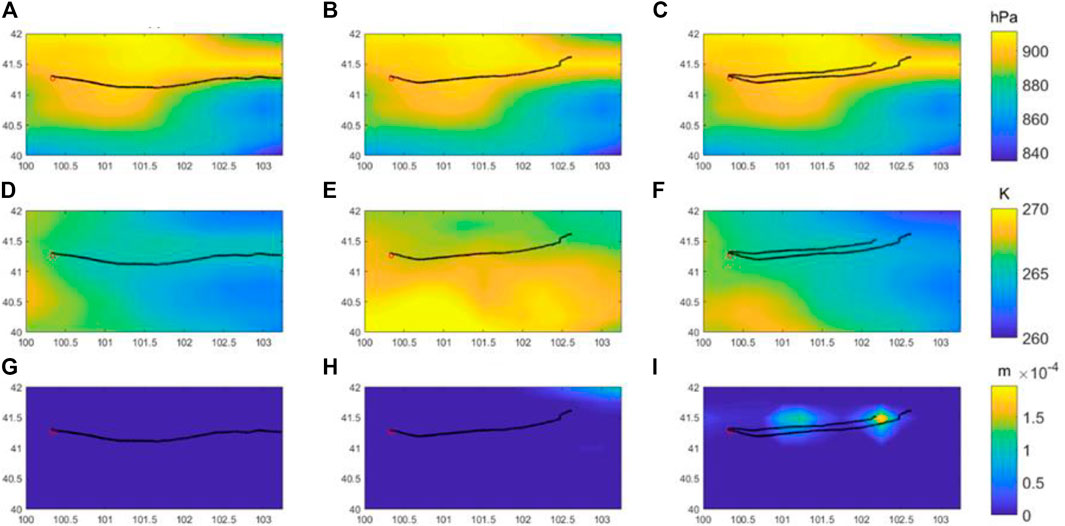
FIGURE 3. The distribution of the meteorological elements around the release point of the sounding balloons from January 13 to 15, where (A–C) are surface air pressure, (D–F) are atmospheric temperature 2 m away from the ground, and (G–I) are total precipitation. The red circle represented the release position of the balloon, and the black point represented the horizontal trajectory of the balloon.

FIGURE 4

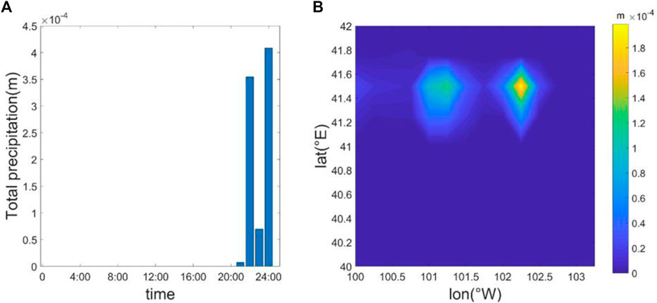
FIGURE 4. The precipitation data on January 15, where (A) shows the hourly precipitation in the target area, and (B) shows the distribution of precipitation from 20:00 to 24:00.

Figure 4 shows the 4-h precipitation data on January 15. As can be seen from Figure 4, precipitation mainly concentrated at 20:00–24:00, and large-scale turbulence in the stratosphere existed before and during the precipitation. Analyzing the generation mechanism of turbulence, there are three main types of turbulence generated in the atmosphere. One is convective turbulence, which is generated by static instability of the atmosphere and its energy source is buoyancy work. The second is mechanical turbulence, which is caused by wind edging. The energy source is shear force work. The third is the turbulence caused by the breaking of gravity wave. When the amplitude of gravity wave increases to a certain extent, the breaking occurs and turbulence is generated (He et al., 2020a). In previous research, when precipitation occurs, it is conducive to the upload of gravity wave energy to the stratosphere (Stephan et al., 2016), which has an important impact on the generation of turbulence. Therefore, analyze the vertical distribution of wind shear, buoyancy frequency, and Richardson number at 13:00 and 20:00. The buoyancy frequency $N^2$ is used to characterize the stable state of free atmospheric air particles. When $N^2<0$, the air particles are in a static and unstable state, which is calculated by Eqs 2, 3. As precipitation is involved, the calculation method of buoyancy frequency of saturated wet air proposed by Wilson et al. in 2013 is used. Vertical wind shear can be calculated by

$\begin{array}{c}\mathbf{S}\mathbf{h}\mathbf{e}\mathbf{a}\mathbf{r}\mathbf{s}=\sqrt{{\left(\frac{\mathbf{\partial }\mathbf{u}}{\mathbf{\partial }\mathbf{z}}\right)}^2+{\left(\frac{\mathbf{\partial }\mathbf{v}}{\mathbf{\partial }\mathbf{z}}\right)}^2}\end{array}(7)$

The larger the vertical wind shear, the greater the dynamic instability of the environment. The calculation equation of Richardson number is

$\begin{array}{c}\mathbf{R}\mathbf{i}=\frac{\overline{{\mathbf{N}}^2}}{{\left(\frac{\mathbf{\partial }\overline{\mathbf{u}}}{\mathbf{\partial }\mathbf{z}}\right)}^2+{\left(\frac{\mathbf{\partial }\overline{\mathbf{v}}}{\mathbf{\partial }\mathbf{z}}\right)}^2}\end{array}(8)$

It reflects the ratio of the buoyancy work to the work by shear force. When Richardson number is less than the critical value 0.25, the atmosphere is unstable and turbulence is more likely to occur. To observe the relationship more intuitively between stratospheric large-scale turbulence and the factors affecting the development of turbulence, wind shear, buoyancy frequency, and Richardson number were calculated. The three factors and Thorpe scale calculated by the two sets of data on January 15 were put into Figure 5, and only the altitude above the tropopause was selected for easy observation.

FIGURE 5

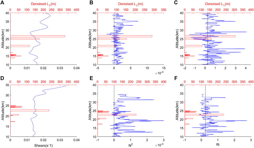
FIGURE 5. The profile of Thorpe scale, Wind shear, Buoyancy frequency, Richardson number above the tropopause (A–C are calculated from sounding data at 13:00; D–F are calculated from sounding data at 20:00; solid red lines are Thorpe scales; solid blue lines from left to right are wind shear, buoyancy frequency and Richardson number).

Figure 5 shows the vertical distribution of Thorpe scale, vertical wind shear, buoyancy frequency, and Richardson number at 13:00 and 20:00 on January 15. Among them, the Thorpe scale of large size appeared at 24.6 and 26.0 km at 13:00, and 22.3 km at 16:00. In the calculation of gradient Richardson number and wind shear, considering the influence of noise, the wind speed is processed by smoothing and undersampling at 30 m. To facilitate observation, Figure 5 shows the data profile after smoothing at 15 points. The smoothing data is only for observation and not used for actual calculation.

It can be seen from Figures 5A, D that the stratospheric wind shear is generally high, all greater than 0.01 s⁻¹, but there are certain oscillations, and local wind shear has a maximum value. The altitude of large Thorpe scale at 13:00 was between the maximum wind shear of 22.2 km and the minimum wind shear of 28.6 km, but there was a small increase of wind shear at the altitude of both Thorpe scales. At 20:00, it is obvious that the maximum value of wind shear appears near 22.3 km, which proves that the increase of shear force work caused by the increase of wind shear has a positive effect on the generation and strengthening of turbulence. Figures 5B, E shows the profile of buoyancy frequency at 13:00 and 20:00 on January 15. The black solid line is the critical value of the buoyancy frequency (taken as 0). It can be seen that the buoyancy frequency in the stratosphere is generally high and the atmospheric instability is reduced. However, in the large-value region of Thorpe scale, such as near 25 km in Figure 5B and near 23 km in Figure 5E, dense negative region of buoyancy frequency appears. It is proved that the unstable region of air particles appears in the Thorpe scale large-value region, which is beneficial to the appearance of turbulence. Figures 5C, F shows the vertical profiles of gradient Richardson number. Same as above, the black solid line is the critical value of Richardson number (taken as 0.25). Richardson number less than 0.25 indicates an increase in the Kelvin Helmholtz instability, which is conducive to the generation of turbulence. It can be seen from the figure that the gradient Richardson number is also small in the large Thorpe scale area, and the Kelvin Helmholtz instability is reduced, which is one of the favorable mechanisms for turbulence. Combining Figures 5B, E and Figures 5C, F, it is found that the small value area of buoyancy frequency and gradient Richardson number is still found in the high-rise area on January 15. The author believes that the detection height is too high in the middle stratosphere. The noise caused by the radiosonde itself increases, which is also shown in the local TNR in Table 2. The flipping caused by this noise has been processed in the calculation of the Thorpe scale.

It can be seen from the above study that the turbulence detected at 13:00 and 20:00 on January 15 has been enhanced in the lower and middle stratosphere, which is shown that the enhancement of turbulence in the middle and lower stratosphere has a clear positive correlation with the precipitation in the troposphere. The remaining seven groups of detection data are analyzed to observe their data characteristics and cumulative distribution of Thorpe scale, as shown in Figure 6.

FIGURE 6

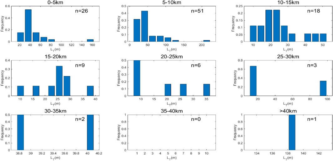
FIGURE 6. Histogram of Thorpe scale frequency distribution per 5 km height for seven sets of sounding data from January 10 to 14.

Figure 6 shows the Thorpe scale distribution calculated from seven groups of radiosonde data from January 10 to 14. To intuitively observe and analyze the local distribution characteristics at different altitudes, the Thorpe scale was divided into nine segments along the altitude, which is listed in the nine frequency distribution histograms. It can be seen from Figure 6 that the turbulence is mostly distributed in the troposphere region (0–10 km), with 77 Thorpe scales in total, accounting for 66.4% of the total Thorpe scales, and there are greater Thorpe scales in the troposphere. Thorpe scales larger than 50 m occupy 27.3% of the total troposphere. The same proportion in the stratosphere is only 7.7%. In addition, Thorpe scale in the middle and upper troposphere (5–10 km) is generally stronger, which is caused by strong convective instability in the middle and upper troposphere and stronger wind shear in the upper troposphere. The amount of turbulence in the stratosphere is small and concentrated in the lower stratosphere. The main reason is that the stability of the free atmosphere increases rapidly in the stratosphere, and most buoyancy frequencies are greater than 0. Although the wind shear in the stratospheric is generally strong, most of the turbulence generated by shear force work is balanced out by stable atmospheric circulation in the stratosphere (Obukhov, 1971; Ko et al., 2019). Therefore, only a few small turbulence layers remain in the stratosphere.

Thorpe scale reflects the intensity of potential temperature reversal caused by turbulence, while turbulence thickness reflects the vertical scale of turbulence layer. Both of them represent the intensity of turbulence. Therefore, the distribution of turbulence thickness is analyzed in the same way, as shown in Figure 7

FIGURE 7

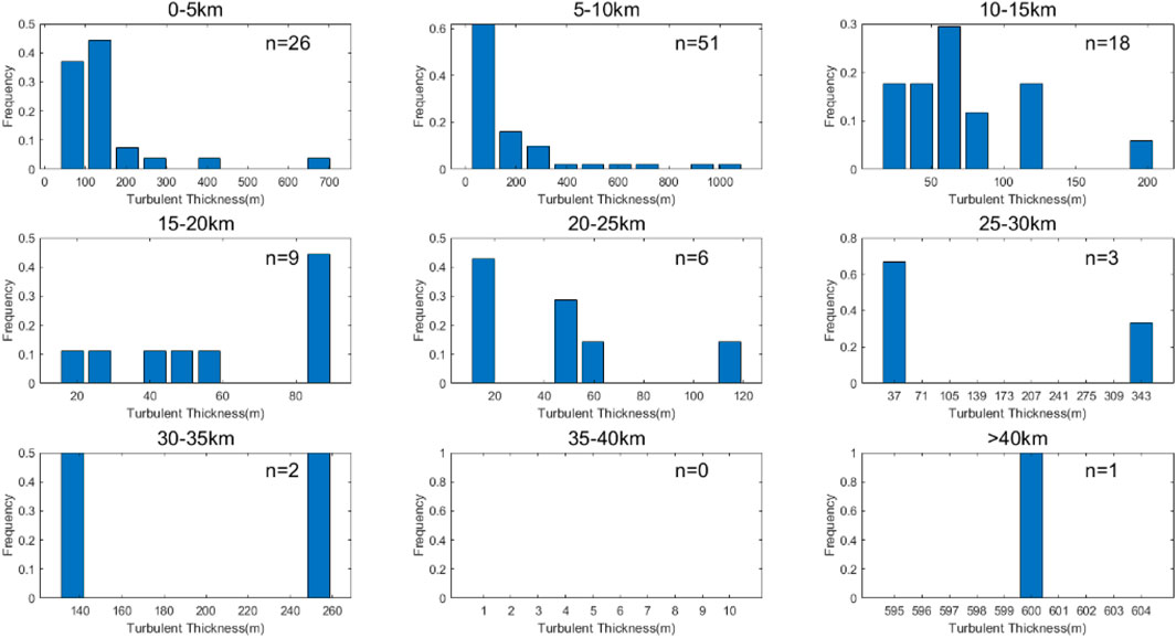
FIGURE 7. Histogram of frequency distribution of turbulence thickness per 5 km height for seven sets of sounding data from January 10 to 14.

Figure 7 shows the frequency distribution histogram of turbulence thickness in each altitude segment obtained from seven sets of sounding data. It can be seen that the distribution of turbulence thickness is roughly the same as that of the Thorpe scale. The turbulence thickness in the troposphere is larger, with the maximum thickness reaching 1.092 km and the average thickness being 177 m. The proportion of turbulence thickness greater than 100 m reached 57%, while the stratospheric turbulence thickness greater than 100 m accounted for only 23%, which was similar to the proportion of turbulence thickness measured by He et al. (2020) in the Hami region of China. Moreover, the maximum turbulence thickness in the stratosphere was 600 m, and the average turbulence thickness was only 90 m. Its distribution is roughly the same as the Thorpe scale. The turbulence thickness and Thorpe scale are both factors that measure the strength of turbulence. The buoyancy frequency of the troposphere is mostly negative, and the gradient Richardson number is generally small. The instability of the internal air particles is stronger, and it is easier to cause a large-scale overturn of the potential temperature, resulting in larger-scale turbulence, which is reflected in the enhancement of Thorpe scale and the turbulence thickness, and the stratosphere stable atmospheric conditions make it not easy to produce massive potential temperature overturn, so only in special circumstances will produce the large-scale turbulence, as was the case with the two sets of radiosonde data discussed above on January 15.

Conventional measurements of turbulent kinetic energy dissipation rate in the global free atmosphere using radiosonde can better understand the spatio-temporal variation of turbulent mixing in the global free atmosphere (Kantha and Hocking, 2011). The turbulent diffusion coefficient is an important parameter needed to simulate the transport of various atmospheric components with small contents in the middle atmosphere (Fukao et al., 1994), both of the two parameters play an important role in the spatio-temporal changes of turbulence. Eq. 4 and Eq. 5 were used to calculate the turbulent kinetic energy dissipation rate and turbulent diffusion coefficient of seven groups of conventional detection data from January 10 to 14, and their vertical distribution was listed in Figure 8.

FIGURE 8

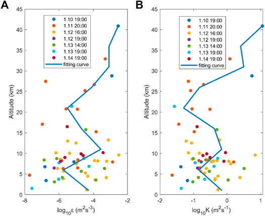
FIGURE 8. The vertical distribution diagram of turbulent kinetic energy dissipation rate and turbulent diffusion coefficient from January 10 to 14, in which the solid blue line is the fitting distribution profile by cubic spline interpolation, (A,B) show the turbulent kinetic energy dissipation rate and turbulent diffusion coefficient respectively.

Figure 8 shows the vertical distribution of the turbulent energy dissipation rate and turbulent diffusion coefficient of seven sets of detection data. To observe the distribution law more intuitively, the seven sets of data are combined and fitted with cubic spline interpolation to obtain the distribution profile. The fitting profile shows that the turbulent energy dissipation rate is generally small in the troposphere. The main reason is that convection instability is higher in the troposphere, buoyancy frequency is small and mostly negative, but it is affected by a strong turbulence layer. When the turbulence layer with large Thorpe scale appears, there will be a local large-value region of ε. It can be seen from Figure 8A that the maximum value of the turbulent kinetic energy dissipation rate appears near the tropopause, which is caused by the jet stream near the tropopause in winter (Fukao et al., 1994), and the release point of the sonde is located in the mountainous plateau region of northwest China. Mountain wave breaking in the tropopause region also results in the enhancement of ε (Lilly and Kennedy, 1973; Zhang et al., 2019). When the height reaches the stratosphere, convective instability decreases, buoyancy frequency increases, and ε increases. Compared with the turbulent kinetic energy dissipation rate, the diffusion coefficient distribution is roughly same in the troposphere. However, according to Eqs 4, 5, it can be seen that the influence of buoyancy frequency on the diffusion coefficient is less than its influence on the kinetic energy dissipation rate. Although the buoyancy frequency of the troposphere is relatively small, the large-scale turbulence layer makes the gas diffusion and transmission stronger, and therefore exhibits a larger K value than the lower stratosphere. And due to the existence of the tropopause jet stream and the breaking of the mountain waves, there is also a local maximum in the K value around the tropopause. As the height increases, the buoyancy frequency gradually increases and the diffusion coefficient increases.

Summary

The Thorpe method has been considered feasible in turbulence detection (Sunilkumar et al., 2015; Martini et al., 2017). In this study, a group of sounding balloons released in Northwest China in January 2018 were analyzed from two aspects: 1) distribution of Thorpe scale and turbulence thickness; 2) distribution and general trend of turbulent kinetic energy dissipation rate and turbulent diffusion coefficient. The results show that there is a certain relationship between stratospheric turbulence and tropospheric precipitation, and fill the gap of higher-altitude turbulence detected by high-resolution sounding balloon in this area.

The troposphere is more prone to turbulence than the stratosphere. Among the turbulence layers that have been detected, turbulence in the troposphere accounts for 66.4% of the total turbulence. The main causes are instability of thermal convection and breaking mountain wave. Owing to the gravity wave breaking caused by wind shear, there will also be a small number of turbulence layers in the stratosphere, but the number is sparse and the intensity is small. The average Thorpe scale in the stratosphere is 28.8 m, which is smaller than the troposphere’s 47.2 m. The intensity distribution of turbulence thickness is roughly the same on the Thorpe scale, and the average turbulence thickness in the troposphere reaches 177 m, which is greater than the average thickness of 90 m in the stratosphere. In terms of the specific altitude, turbulent layer with the highest frequency location is located in the upper troposphere 5–10 km, accounts for 44.0% of the total turbulent layer, the largest Thorpe scale and turbulent layer thickness are also located at this altitude. The main reason is that the release point is located in the mountainous plateau area of northwestern China. The strong topographical gravity waves cause the turbulence near the tropopause to increase significantly. This is consistent with the conclusion that the topography affects turbulence discovered by Zhang et al. (2019). The occurrence of tropopause jet in January in winter also aggravates this phenomenon. The same distribution can be found in the turbulent kinetic energy dissipation rate and diffusion coefficient. Owing to the existence of tropopause jet stream and Kelvin Helmholtz shear instability, the maximum value of ε and K appears near the tropopause at 10 km.

By analyzing the Thorpe scale and turbulence thickness of nine sets of data, it is found that the two sets of sounding data at 13:00 and 20:00 on January 15 have large-scale turbulence near the altitude of 23 km in the middle stratosphere. This is different from the previous study. Analyzing the meteorological elements on the balloon flight path, it was found that there was a certain amount of precipitation on the night of January 15, and the precipitation area was roughly the same as the horizontal trajectory of the balloon flight. It is indicated that the precipitation has a certain relationship with the large-scale turbulence in the middle stratosphere. Before and during the precipitation, a large-scale turbulence appears in the middle stratosphere. This phenomenon has not been mentioned before by the Thorpe method, and we will carry out further investigations on the relationship between turbulence and precipitation in the future.

Author Contributions

ZQ and ZS designed the experiments; ZQ, ZS, YH and YF performed the experiments; ZQ and YH analysed the data; ZQ wrote the paper. All authors have read and agreed to the published version of the manuscript.

Funding

The study was supported by the National Natural Science Foundation of China (Grant 41875045), Hunan Outstanding Youth Fund Project (Grant 2021JJ10048).

Conflict of Interest

The authors declare that the research was conducted in the absence of any commercial or financial relationships that could be construed as a potential conflict of interest.

Publisher’s Note

All claims expressed in this article are solely those of the authors and do not necessarily represent those of their affiliated organizations, or those of the publisher, the editors and the reviewers. Any product that may be evaluated in this article, or claim that may be made by its manufacturer, is not guaranteed or endorsed by the publisher.

Acknowledgments

“Western Light’’ Cross-Team Project of the Chinese Academy of Sciences, Key Laboratory Cooperative Research Project.

References

Bellenger, H., Wilson, R., Davison, J. L., Duvel, J. P., Xu, W., Lott, F., et al. (2017). Tropospheric Turbulence over the Tropical Open Ocean: Role of Gravity Waves. J. Atmos. Sci. 74 (4), 1249–1271. doi:10.1175/JAS-D-16-0135.1

CrossRef Full Text | Google Scholar

Chen, F., and Avissar, R. (1994). Impact of Land-Surface Moisture Variability on Local Shallow Convective Cumulus and Precipitation in Large-Scale Models. J. Appl. Meteorol. Climatol. 33, 1382–1401. doi:10.1175/1520-0450(1994)033<1382:iolsmv>2.0.co;2

CrossRef Full Text | Google Scholar

Clayson, C. A., and Kantha, L. (2008). On Turbulence and Mixing in the Free Atmosphere Inferred from High-Resolution Soundings. J. Atmos. Ocean Technol. 25 (6), 833–852. doi:10.1175/2007JTECHA992.1

CrossRef Full Text | Google Scholar

Cohn, S. A. (1995). Radar Measurements of Turbulent Eddy Dissi- Pation Rate in the Troposphere A Comparison of Techniques. Atmos. Ocean. Technol. 12, 85. doi:10.1175/1520-0426(1995)012<0085:rmoted>2.0.co;2

CrossRef Full Text | Google Scholar

Collow, T. W., Robock, A., and Wu, W. (2014). Influences of Soil Moisture and Vegetation on Convective Precipitation Forecasts Over the United States Great plains. J. Geophys. Res. Atmos. 119 (15), 9338–9358. doi:10.1002/2014JD021454

CrossRef Full Text | Google Scholar

Dale, R., and Durran, J. B. K. (1982). On the Effects of Moisture on the Brunt-Visl Frequency. J. Atmos. Sci. 39, 2152. doi:10.1175/1520-0469(1982)039<2152:oteomo>2.0.co;2

CrossRef Full Text | Google Scholar

Fritts, D. C., Wan, K., Franke, P. M., and Lund, T. (2012). Computation of clear-air Radar Backscatter from Numerical Simulations of Turbulence: 3. Off-Zenith Measurements and Biases throughout the Lifecycle of a Kelvin-Helmholtz Instability. J. Geophys. Res. 117, B17101. doi:10.1029/2011JD017179

CrossRef Full Text | Google Scholar

Fritts, D. C., and Werne, J. A. (2000). Turbulence Dynamics and Mixing Due to Gravity Waves in the Lower and Middle Atmosphere. Geophys. Monogr. Ser. 123, 143–159. doi:10.1029/GM123p0143

CrossRef Full Text | Google Scholar

Fukao, S., Yamanaka, M. D., Ao, N., Hocking, W. K., Sato, T., Yamamoto, M., et al. (1994). Seasonal Variability of Vertical Eddy Diffusivity in the Middle Atmosphere 1. Three-Year Observations by the Middle and Upper Atmosphere Radar. J. Geophys. Res. 99 (D9), 18973. doi:10.1029/94jd00911

CrossRef Full Text | Google Scholar

He, Y., Sheng, Z., and He, M. (2020a). The First Observation of Turbulence in Northwestern China by a Near-Space High-Resolution Balloon Sensor. Sensors 20, 677. doi:10.3390/s20030677

PubMed Abstract | CrossRef Full Text | Google Scholar

He, Y., Sheng, Z., Zhou, L., He, M., and Zhou, S. (2020b). Statistical Analysis of Turbulence Characteristics over the Tropical Western pacific Based on Radiosonde Data. Atmosphere 11 (4), 386. doi:10.3390/ATMOS11040386

CrossRef Full Text | Google Scholar

Hersbach, H., Bell, B., Berrisford, P., Hirahara, S., Horányi, A., Muñoz‐Sabater, J., et al. (2020). The ERA5 Global Reanalysis. Q.J.R. Meteorol. Soc. 146 (730), 1999–2049. doi:10.1002/qj.3803

CrossRef Full Text | Google Scholar

Hooper, D. A., and Thomas, L. (1998). Complementary Criteria for Identifying Regions of Intense Atmospheric Turbulence Using Lower VHF Radar. J. Atmos. Sol.-Terr. Phys. 60 (1), 49–61. doi:10.1016/s1364-6826(97)00054-0

CrossRef Full Text | Google Scholar

Jonko, A. K., Yedinak, K. M., Conley, J. L., and Linn, R. R. (2021). Sensitivity of Grass Fires Burning in Marginal Conditions to Atmospheric Turbulence. J. Geophys. Res. Atmos. 126, e2020JD033384. doi:10.1029/2020JD033384

CrossRef Full Text | Google Scholar

Kantha, L., and Hocking, W. (2011). Dissipation Rates of Turbulence Kinetic Energy in the Free Atmosphere: MST Radar and Radiosondes. J. Atmos. Sol.-Terr. Phys. 73 (9), 1043–1051. doi:10.1016/j.jastp.2010.11.024

CrossRef Full Text | Google Scholar

Ko, H.-C., and Chun, H.-Y. (2022). Potential Sources of Atmospheric Turbulence Estimated Using the Thorpe Method and Operational Radiosonde Data in the United States. Atmos. Res. 265, 105891. doi:10.1016/j.atmosres.2021.105891

CrossRef Full Text | Google Scholar

Ko, H. C., Chun, H. Y., Wilson, R., and Geller, M. A. (2019). Characteristics of Atmospheric Turbulence Retrieved from High Vertical‐Resolution Radiosonde Data in the United States. J. Geophys. Res. Atmos. 124 (14), 7553–7579. doi:10.1029/2019JD030287

CrossRef Full Text | Google Scholar

Kohma, M., Sato, K., Tomikawa, Y., Nishimura, K., and Sato, T. (2019). Estimate of Turbulent Energy Dissipation Rate from the VHF Radar and Radiosonde Observations in the Antarctic. J. Geophys. Res. Atmos. 124 (6), 2976–2993. doi:10.1029/2018JD029521

CrossRef Full Text | Google Scholar

Lilly, D. K., and Kennedy, P. J. (1973). Observations of a Stationary Mountain Wave and its Associated Momentum Flux and Energy Dissipation. J. Atmos. Sci. 30, 1135. doi:10.1175/1520-0469(1973)030<1135:ooasmw>2.0.co;2

CrossRef Full Text | Google Scholar

Martini, E., Freni, A., Cuccoli, F., and Facheris, L. (2017). Derivation of Clear-Air Turbulence Parameters from High-Resolution Radiosonde Data. J. Atmos. Ocean. Technol. 34 (2), 277–293. doi:10.1175/JTECH-D-16-0046.1

CrossRef Full Text | Google Scholar

Obukhov, A. M. (1971). Turbulence In An Atmosphere With A Non-Uniform Temperature. Bound.-Layer Meteorol. 2, 7. doi:10.1007/bf00718085

CrossRef Full Text | Google Scholar

Riley, J. J., and Lindborg, E. (2008). Stratified Turbulence: A Possible Interpretation of Some Geophysical Turbulence Measurements. J. Atmos. Sci. 65 (7), 2416–2424. doi:10.1175/2007JAS2455.1

CrossRef Full Text | Google Scholar

Riveros, H. G., and Riveros-Rosas, D. (2010). Laminar and Turbulent Flow in Water. Phys. Educ. 45, 288–291.

CrossRef Full Text | Google Scholar

Sharman, R. D., Trier, S. B., Lane, T. P., and Doyle, J. D. (2012). Sources and Dynamics of Turbulence in the Upper Troposphere and Lower Stratosphere: A Review. Geophys. Res. Lett. 39, L12803. doi:10.1029/2012GL051996

CrossRef Full Text | Google Scholar

Stephan, C. C., Joan Alexander, M., Hedlin, M., de Groot-Hedlin, C. D., and Hoffmann, L. (2016). A Case Study on the Far-Field Properties of Propagating Tropospheric Gravity Waves. Mon. Weather Rev. 144 (8), 2947–2961. doi:10.1175/MWRD-16-0054.1

CrossRef Full Text | Google Scholar

Sun, Z., Ning, H., Song, S., and Yan, D. (2016). First Observations of Elevated Ducts Associated with Intermittent Turbulence in the Stable Boundary Layer over Bosten Lake, China. J. Geophys. Res. Atmos. 121 (19), 201–211. doi:10.1002/2016JD024793

CrossRef Full Text | Google Scholar

Sunilkumar, S. v., Muhsin, M., Parameswaran, K., Venkat Ratnam, M., Ramkumar, G., Rajeev, K., et al. (2015). Characteristics of Turbulence in the Troposphere and Lower Stratosphere over the Indian Peninsula. J. Atmos. Sol.-Terr. Phys. 133, 36–53. doi:10.1016/j.jastp.2015.07.015

CrossRef Full Text | Google Scholar

Thorpe, S. A. (1977). Turbulence and Mixing in a Scottish Loch. Philos. Trans. Roy. Soc. 286, 125. doi:10.1098/rsta.1977.0112

CrossRef Full Text | Google Scholar

Wilson, R., Dalaudier, F., and Luce, H. (2011). Can One Detect Small-Scale Turbulence from Standard Meteorological Radiosondes? Atmos. Meas. Tech. 4 (5), 795–804. doi:10.5194/amt-4-795-2011

CrossRef Full Text | Google Scholar

Wilson, R., Luce, H., Dalaudier, F., and Lefrère, J. (2010). Turbulence Patch Identification in Potential Density or Temperature Profiles. J. Atmos. Ocean. Technol. 27 (6), 977–993. doi:10.1175/2010JTECHA1357.1

CrossRef Full Text | Google Scholar

Wilson, R. (2004). Turbulent Diffusivity in the Free Atmosphere Inferred from MST Radar Measurements: A Review. Ann. Geophys. 22 (11), 3869–3887. doi:10.5194/angeo-22-3869-2004

CrossRef Full Text | Google Scholar

Zhang, J., Zhang, S. D., Huang, C. M., Huang, K. M., Gong, Y., Gan, Q., et al. (2019). Latitudinal and Topographical Variabilities of Free Atmospheric Turbulence from High‐Resolution Radiosonde Data Sets. J. Geophys. Res. Atmos. 124 (8), 4283–4298. doi:10.1029/2018JD029982

CrossRef Full Text | Google Scholar

Zhou, (2018). Detection and Analysis of clear Air Turbulence in the Middle Atmosphere. PhD dissertation. Changsha (China): National University of Defense Technology.

Google Scholar