- 1School of Economics, Zhengzhou University of Aeronautics, Zhengzhou, China
- 2Post-Doctoral Moving Station of Applied Economics, Henan University, Kaifeng, China
- 3School of Economics, Zhongnan University of Economics and Law, Wuhan, China
From the perspective of input and output differentiation, using the SBM directional distance function method and Luenberger productivity index, this paper calculates the index of the green total factor productivity (GTFP) growth of 280 cities in China, from 2004 to 2016. This study also analyzes the growth sources of urban GTFP and the decomposition situation of GTFP in four cases, as well as the factors that affect the growth of GTFP. Finally, the following conclusions are drawn: 1) the overall growth trend of GTFP under four different situations of elements input is basically consistent. As a whole, the growth trend can be divided into three stages. The first rising stage of GTFP growth was from 2004 to 2008; the next declining stage was from 2008 to 2012, and a further rising stage occurred from 2012 to 2016. 2) From the decomposition situation of GTFP growth, we can know that the main source of GTFP growth is in the scale efficiency (LSEC) of GTFP. The decomposition of inefficiency levels in four cases shows that the inefficiency of land resources is the highest among many factors. Land resource inefficiency is also the key factor determining the output efficiency; the input inefficiency and bad-output inefficiency between them account for about 50% of the overall inefficiency level. 3) Among the factors that influence GTFP growth, the negative effect of urban land and energy structure is mainly reflected in the pure technology growth (LPTP) and scale efficiency growth (LSEC) of GTFP. In addition, investment in scientific and technological innovation and foreign direct investment both have a significantly positive effect on GTFP growth, as well as in improving urban population density and road area per capita.
Introduction
Energy has become an important factor affecting the improvement of economic efficiency and high-quality development of China’s economy. In fact, during the 11th Five-Year Plan period (2005–2010), China’s energy consumption per unit GDP actually decreased by 19.3%. The actual decline was 18.4% during the 12th Five-Year Plan period (2010–2015), and the ratio of energy consumption per unit GDP decreased by 11.4% from 2015 to 2018, during the 13th Five-Year Plan period. Energy consumption has decreased more than before, but it is still one of the important factors that cannot be ignored in the process of high-quality economic development (970 million tons of coal, 49.18 million tons of crude oil, and 53.3 billion cubic meters of natural gas were produced in China in the first quarter of 2021, based on National Bureau of Statistics data).
At the same time, the rapid development of urbanization in China has caused urban land resources to be a core element of economic development. By the end of 2018, the number of Chinese cities had reached 672 (297 prefecture-level cities; 375 county-level cities). The urbanization rate of permanent residents reached 59.58% (48.94% higher than in 1949); at the end of 1978, there were 193 cities (101 prefecture-level cities; 92 county-level cities). During this period, specifically from 1981 to 2017, the urban built-up area in China increased from 7,438 km2 to 56,225 km2, an increase of nearly 660%, based on data from the National Bureau of Statistics in China.
The rapid growth and high-quality development of China’s economy have also been closely related to the process of market-oriented reform (Cai, 2018; Liu, 2018) and the degree of market resource allocation (Nie and Jia, 2011). However, existing research on resource allocation focuses more on capital elements (Chen et al., 2019; Wu and Lin, 2016; Fang, 2007) and human capital elements (Li and Yin, 2017; Yuan and Xie, 2011; Lai and Ji, 2015), as well as on the matching degree of capital and labor (Hsieh and Klenow, 2009). Some studies have focused on the allocation of resources for the agricultural (Elahi et al., 2021a; Elahi et al., 2021b), industrial sectors (Zhao et al., 2021; Sun et al., 2021c; Pei et al., 2020), energy efficiency (Sun et al., 2021a; Zhang et al., 2021), or socio-economic viability of solar commercialization and electrification (Sun et al., 2021a) and the effect of technological innovation and knowledge spillover on energy efficiency (Sun et al., 2021b). But only a few scholars have put energy factors into a production function model in the overall analysis of resource allocation efficiency (Wang et al., 2010; Chen and Chen, 2017; Watanabe and Tanaka, 2007; Sun et al., 2021c), mostly focus on labor, capital, technology, and other factors (Wang et al., 2006; Cai and Fu, 2017). Therefore, this paper will mainly focus on the effect of energy and land resource factors on the green total factor productivity (GTFP) when considering capital, labor, energy and land factors (K/L/E/S), as well as considering the environment factors, which is different from traditional productivity analyses that only consider capital and labor (K/L).
As for the measurement of GTFP, the global SBM directional distance function is the mainstream method used to measure productivity (Tone, 2001; Fukuyama and Weber, 2009; Yang et al., 2019). Yang et al. (2019) measured using the Malmquist-Luenberger index (Fare et al., 1994; Chung and Fare, 1995), based on the non-radial slack SBM direction distance function (Tone, 2001). The index was then decomposed into an efficiency change index (ML-EFFCH) and technology change index (ML-TECH). Many scholars have used the Malmquist-Luenberger index (Chung and Fare, 1995) to measure the green total factor productivity in the United States (Fare et al., 2001), OECD countries, Asia (Jeon & Sickles, 2004), Taiwan Province (Yu et al., 2008), OPEC countries (Wang et al., 2008) and China (Kaneko and Managi, 2004; Managi and Kaneko, 2006; Yang and Shao, 2009; Chen, 2010).
Liu et al. (2016) calculated the GTFP and its decomposition value based on the DEA-Malmquist productivity index. The study took SO2 and COD emissions as environmental bad output factors. Chen (2016) calculated the industrial GTFP by using the SBM directional distance function and ML index. Wang et al. (2010) analyzed and decomposed the GTFP using the SBM directional distance function and Luenberger productivity index. The study found that excessive energy consumption and excessive emissions of SO2 and COD would lead to environmental inefficiency. Dong et al. (2012) measured the source of industrial GTFP by using slack efficiency loss and the Luenberger productivity index. The study found that both labor technology progress (Li and An, 2012) and pollution control (Wang and Sheng, 2015) can effectively improve industrial GTFP. Kuang and Peng (2012), using the Malmquist index combined with stochastic frontier function in a VRS case, found that GTFP can reflect environmental efficiency loss and resource utilization efficiency differences. Cui and Zhang (2014) measured China’s agricultural environmental efficiency and agricultural green total factor productivity, as well as their changes, based on the principle of material conservation. The results showed that environmental efficiency can reflect the utilization efficiency and material absorption efficiency of various factors in agricultural production.
In the process of measuring GTFP, environmental factors must be included in the input-output production function. These factors may accurately measure the loss of efficiency of resources. Some scholars regard energy as an environmental resource input (Chen and Chen, 2017; Watanabe and Tanaka, 2007; Tone, 2001; Fukuyama and Weber, 2009; Yang and Shao, 2009). Some scholars also divide “good output” and “bad output” in resource output to measure the influence of environmental factors. The measurement of bad output is usually set by three industrial wastes, namely industrial waste gas, smoke and water emissions (Cheng and Li, 2009; Hu et al., 2008; Wu, 2010; Kaneko and Managi, 2004; Managi and Kaneko, 2006). Others only use SO2 emissions (TuWatanabe and Tanaka, 2007; TuWatanabe and Tanaka, 2008), or add COD based on the former (Managi and Kaneko, 2006; Hu et al., 2008; Wang et al., 2010), or CO2 emissions (Yang et al., 2019).
Based on the above analysis, the main contributions of this paper are as follows: Firstly, this paper will mainly focus on the effect of energy and land resource factors on the green total factor productivity (GTFP) when considering capital, labor, energy and land factor (K/L/E/S), which is different from traditional productivity analyses that only consider capital and labor (K/L). Secondly, using the method of SBM directional distance function and Luenberger productivity index from the perspective of resource input-output differentiation, it calculates the index of the GTFP growth of 280 cities in China from 2004 to 2016, and analyzes the growth sources of urban GTFP and the decomposition situation of GTFP in four cases. Thirdly, the study also conducts an inefficiency level analysis of input inefficiency
Theoretical Analysis
The measurement and theoretic analysis of GTFP is mainly based on the Solow economic growth model or its related production function model. The traditional Solow economic growth model mainly covers two production factors: labor (L) and capital (K). The model’s production function is Y=F (A, K, L), which can be further simplified to Y=F (K, AL); AL represents effective labor. Romer (2001) further expanded the model in the book Advanced Macroeconomics, adding natural resources and land resources to the production function, and using the C-D production function model as follows:
In the above formula, K represents capital stock, R represents available resources, T represents available land resources, and α, β, and γ represent corresponding capital elasticity, resource elasticity and land elasticity, respectively. It is also assumed that the scale effect remains unchanged. Next, A and L represent knowledge capital and labor. However, the model only exists in the theoretical analysis level, without any actual measurement analysis.
In the process of studying economic growth and the allocation of resource elements, some scholars consider adding energy elements into the basic AK model Y=F (K, AL), in order to study the phenomenon of total factor productivity or resource mismatch (Pang, 2009; Wang et al., 2010; Yang et al., 2015; Chen and Chen, 2017; Yang et al., 2019). Among them, Chen and Chen (2017) put energy elements into the production function framework and analyzed the total energy elements covering time, industry and region.
The function is set as follows:
where i and j represent different regions and industry sectors;
In this paper, the influence of energy and land factors on the growth of total factor productivity is considered in the model construction. In addition, referring to Brandt’s model construction ideas (Brandt et al., 2013), the growth and change of GTFP in China are analyzed from the allocation efficiency perspective of incorporating energy (E) and land resources (S). Therefore, the theoretical analysis model of this paper is set as follows:
In the above, i represents different urban areas, E represents the amount of energy used, S represents the land resources used, and α, β and γ represent the corresponding elasticity and scale effect. Next,
where,
Then,
As the optimal conditions for maximizing output are:
Then, according to the optimal condition
Then:
Then, the efficiency loss d of resource allocation is obtained:
According to the above analysis, if the energy factor E and land factor S are ignored in
The two conditions need to be met at the same time in ideal conditions, and the realistic conditions only need to meet the first condition. In addition, the process of resource allocation is to make the ratio of various resources infinitely close to the ideal condition
Research Design and Data Description
The data of this paper come from the Statistical Database of China Economic Network and the 《database of the development research center of the State Council. In this paper, the SBM directional distance function and Luenberger productivity indicator are used to measure the GTFP of 280 cities in China, from 2004 to 2016. The production input element and the “good” output elements (for desirable outputs) and “bad” output elements (for undesirable outputs) should also be considered simultaneously (Wang et al., 2010; Yang et al., 2019; Chambers et al., 1996; Caves et al., 1982; Grosskopf, 2003; Yuan and Li, 2018). The factor input in this paper covers four production factors (capital, labor, energy, and land, or K/L/E/S). Outputs include “good” outputs (GDP) and “bad” outputs (three types of industrial waste), with specific indicators as follows: 1) Capital input: capital investment in urban fixed assets investment (unit: 10,000 yuan); 2) Labor input: the number of employees in the city at the end of the year (unit: 10,000 people); 3) Energy input: In the calculation process of total factor productivity, it is necessary to consider energy input. In this paper, the main energy consumption in the city is summed up, and the main energy consumption indexes are the consumption of urban liquefied petroleum gas, natural gas and electricity. Then, according to the conversion coefficient in Table 1, the heat data (KJ) and standard coal (kg) data are obtained. The heat data (KJ) is used as the energy input index, and then the standard coal (kg) input is used as an alternative variable to test the reliability of the index; 4) Land resources input: The urban construction land area can better reflect the supply status of land resources elements in market economy activities and conform to the land’s characteristics as a factor of production. Therefore, the investment of land resources elements is measured by urban construction area (unit: km2); 5) Good output: Good output (also referred to as desirable output) mainly uses industrial added value (Tu, 2008; Yang et al., 2019) or regional GDP (Managi and Kaneko, 2006; Wang et al., 2010). This paper takes cities as the basic unit, so good output is measured by urban GDP (unit: 10,000 yuan); 6) Bad output: The indicators of bad output (also referred to as undesirable output) in this paper are industrial waste gas SO2 (Unit: t), industrial smoke dust (Unit: t) and industrial wastewater discharge (unit: 10,000 t). These three indicators are the main indicators used to measure objects of bad output in the production process (Kaneko and Managi, 2004; Managi and Kaneko, 2006; Hu et al., 2008; Cheng and Li, 2009; Wu, 2010). The data are also relatively complete.
In this paper, every city (with a city as the basic unit) is set as a production decision-making unit (DMU) to construct the production practice boundary. Because different resource elements (labor L, capital K, land S and energy E) need to be incorporated into the production decision-making behavior, it is necessary to construct the environmental factor input (EI), environmental “good” output and “bad” output, including the city K and period T, in the model setting.
In the model, it is assumed that city K uses N kinds of elements as inputs X,
where
In this paper, the global SBM directional distance function (Tone, 2002; Fukuyama and Weber, 2009; Wang et al., 2010; Yang et al., 2019) is used; the specific method is as follows:
In the above,
When the direction vector (
The inefficiency of the input:
The inefficiency of “good” output (for desirable outputs):
The inefficiency of “bad” output (for undesirable outputs):
According to the above method, the inefficiency index of production activities in 280 cities in China, from 2004 to 2016, is calculated in a directional distance function measure, and the 2003 data is the base period data.
The Luenberger productivity index (Chambers et al., 1996) and the Malmquist productivity index (Caves et al., 1982) are applied in different disciplines. Together, they form a Malmquist Luenberger index (ML index) (Chung and Fare, 1995) in the process of development. A Luenberger productivity index is the general form of the M index and ML index, and the specific Luenberger model (Chambers et al., 1996; Wang et al., 2010) is as follows:
Then, according to the idea of Grosskopf (2003), the specific Luenberger model is divided into four parts (Fare et al., 1994; Fare et al., 2007; Wang et al., 2010; Yuan and Li, 2018), which are pure efficiency change (LPEC), pure technology change (LPTP), scale efficiency change (LSEC) and technology pure scale change (LTPSC), as follows:
In the above, if GTFP, LPEC, LPTP, LSEC and LTPSC are greater than (or less than) 0, that indicates that productivity increases (declines), efficiency improves (deteriorates), technology progresses (declines), scale efficiency increases (declines), and technology deviates from CRS.
Empirical Analysis
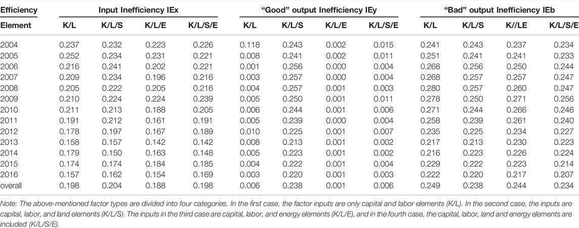
Table 2 lists the decomposition status of inefficiency levels in four cases (K/L; K/L/S; K/L/E, and K/L/S/E). In the input inefficiency (
In the “good” output inefficiency (
In the “bad” output inefficiency (
For better analysis on the proportional relationship between the three inefficiency levels (
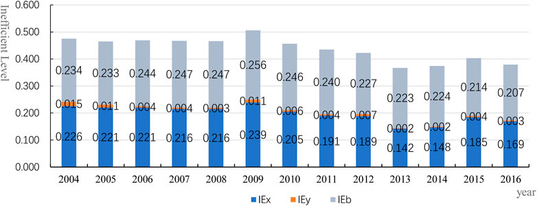
FIGURE 1. Inefficiency levels in fourth case (K/L/S/E) when the capital, labor, land and energy elements are all included.
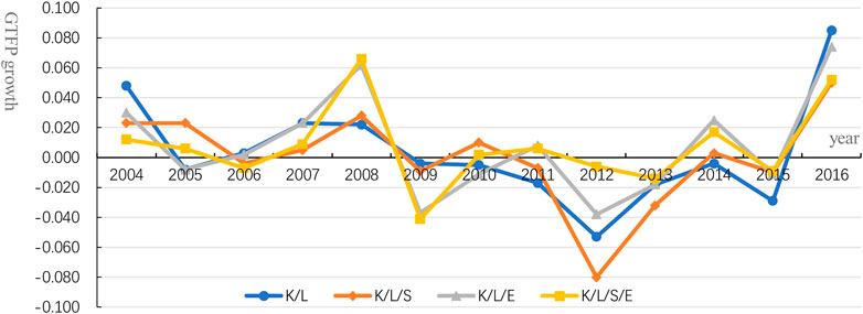
Figure 2 shows the growth of GTFP under four cases (K/L; K/L/S; K/L/E; K/L/S/E). The overall growth trend of GTFP under different situations is basically consistent, and the trend can be divided into three stages as a whole. Specifically, the GTFP growth rate during 2004–2008 was in a rising stage. From 2008 to 2012, the GTFP growth rate was in a declining stage. The GTFP growth rate in 2012–2016 was in a further rising stage. However, in general terms regarding the positive and negative growth rate of GTFP, the rate was positive in the 2004–2008 period, negative in 2009–2015, and positive after 2015.
From 2004 to 2008, the GTFP showed an overall growth trend and a positive value. This was closely related to the opening up of China’s economy and the reform of the domestic market economy (reform and opening up in 1978; market economy reform in the 1990s; China joined the WTO in 2001), which accelerated the transformation and development of China’s economic structure and improved the country’s environmental and economic efficiency. The negative growth rate of GTFP from 2008 to 2015 shows that the “three high effects” of economic structure were prominent (high input, high consumption and high pollution in the production process). The inefficiency of some enterprises with backward production capacity significantly reduced the ecological environment efficiency in urban areas and accelerated the process of environmental pollution and the waste of resources. However, the negative growth trend of the growth rate weakened and began to move towards a positive growth trend in 2012. This changing trend indicated that the effects of environmental protection policies (such as eco-environmental protection, pollution control, waste gas treatment, environmental regulation, waste recovery systems, etc.) began to appear. Then, the production process began to pay more attention to eco-economic concepts, such as low carbon, environmental protection, energy saving, resource saving technological innovation, and harmony between man and nature.
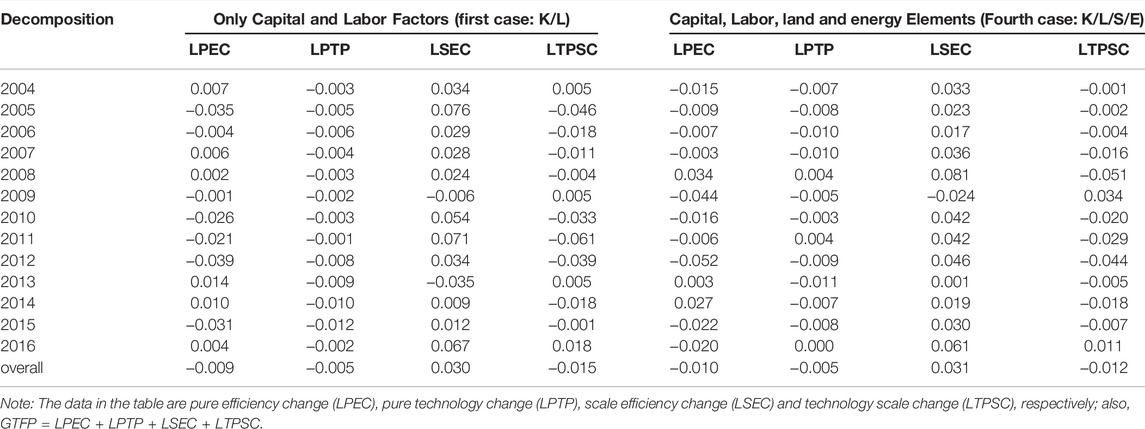
Figure 3 shows the decomposition of the overall GTFP from 2004 to 2016, under four different factor input cases. The four kinds of decomposition results correspond to the overall productivity growth (GTFP). The four kinds of decomposition results are pure efficiency growth (LPEC), pure technology growth (LPTP), scale efficiency growth (LSEC) and technology pure scale growth (LTPSC), which occur in the process of GTFP growth. As can be seen from Figure 3, the GTFP and its decomposition are similar in a growing trend on the whole, but there are some differences in the four different type cases. The GTFP growth rate is the lowest when the land factor is included (second case: K/L/S), and therefore, the land resource factor is the main factor limiting the overall growth of GTFP.
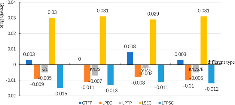
FIGURE 3. Growth rate and decomposition results of overall GTFP in four cases (K/L; K/L/S; K/L/E; K/L/S/E).
In the decomposition of the GTFP growth rate, only LSEC is significantly positive. Pure efficiency growth (LPEC), pure technology growth (LPTP) and technology scale growth (LTPSC) are all significantly negative, indicating that the main source of the green total factor growth rate lies in scale efficiency (LSEC). Meanwhile, pure efficiency, pure technology and technology scale are significantly reducing the overall level of green environment total factor productivity. Taking the fourth case (K/L/S/E) as an example, the scale efficiency growth (LSEC) reaches 0.031; the absolute value is nearly three times that of the pure efficiency growth (LPEC), the value of which is -0.010. Also, pure technology growth (LPTP) is -0.005, and technology scale growth (LTPSC) is -0.012.
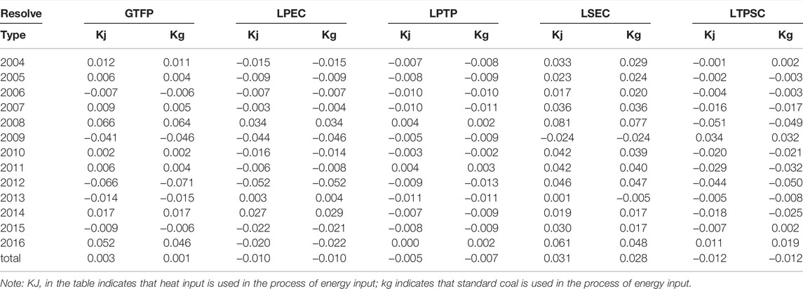
The results in Table 3 show the growth decomposition results of GTFP in different years. The overall decomposition results in two cases are close, and the differences between different growth decomposition types are small. Compared with the first case (K/L), in the fourth case (K/L/S/E), the average value of LPEC is about 0.001 lower than the first case (-0.009 and -0.010 respectively). The average value of LPTP is all -0.005, and the average value of LSEC in the fourth case is 0.001 higher (0.030 and 0.031, respectively). Also, the technology scale growth (LTPSC) is about 0.003 higher (-0.015 and -0.012, respectively), indicating that scale effect is the main source of GTFP growth. In addition, the technology scale (LTPSC) has the greatest negative impact on growth, while scale efficiency (LSEC) has the greatest positive impact. Table 4 shows the decomposition results by using different energy accounting methods. The results are close, similar and robust.
Analysis of the Influencing Factors of GTFP Growth
The above has analyzed the growth process and decomposition situation of GTFP. Next, this study will deeply explore the core factors that affect the growth of GTFP and will analyze the mechanism and process related to GTFP growth. The model of influencing factor analysis is set as follows:
The explained variable (
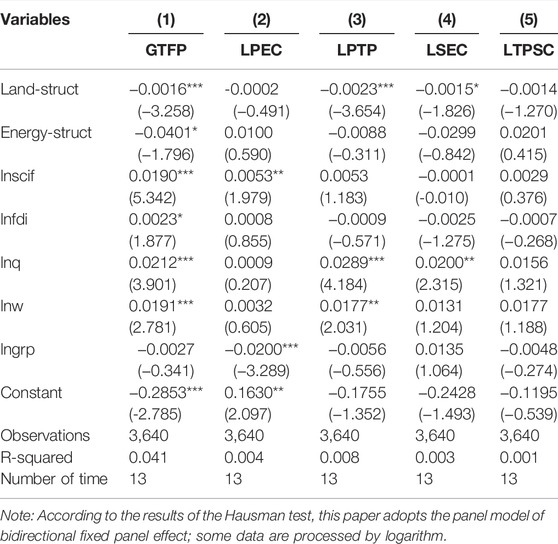
Definition of variables in Function 20 are shown in Table 5. The analysis results of influencing factors are shown in Table 6. As a whole, the greater the proportion of the land construction area is in an urban area, the lower the utilization efficiency of land resources is; the corresponding growth ability of GTFP is also weakened. The overall negative effect is significant at 1% level (the coefficient is -0.0016). This is mainly reflected in pure technology change LPTP (the coefficient is -0.0023) and scale efficiency change LPEC (the coefficient is -0.0015). The overall negative effect of urban energy consumption structure on GTFP growth is significant (the coefficient is -0.0401), but the positive effect on pure efficiency growth (LPEC) and technology scale growth (LTPSC) is not significant. Negative effects are mainly reflected in pure technology change (LPTP) and scale efficiency change (LSEC), but the effect is not significant. This finding shows that no scale effect exists when electricity is the core of energy consumption; the improvement of energy efficiency is also not obvious.
In addition, a 1% growth in innovation investment of local fiscal expenditure on scientific undertakings will promote the growth of GTFP by 0.0190 as a whole. This is mainly due to the increase of LPEC on GTFP (the coefficient is 0.0053). This finding indicates that investment in scientific and technological innovation can improve the production process and production efficiency of enterprises, and then enhance the growth of GTFP. Foreign direct investment has a positive effect on GTFP growth (the coefficient is 0.0023), which shows that foreign investment can bring about a significant improvement in production efficiency. The overall efficiency promotion effect is also higher than that of the “pollution paradise effect”. In addition, for a 1% growth in urban population density and road area per unit owned by urban settlements, the growth effects on GTFP are 0.0212 and 0.0191, respectively.
Conlcusions and Policy Recommendations
From the perspective of resource input-output differentiation, the growth index of green total factor productivity (GTFP) of 280 cities in China, from 2004 to 2016, is calculated by using SBM directional distance function and the Luenberger productivity index. This study also analyzes the growth of urban GTFP and the decomposition situation of overall GTFP in four cases, as well as the factors that affect GTFP growth. The following conclusions are drawn:
1) The overall growth trend of GTFP under four different situations is basically consistent and can be divided into three stages. The growth rate of GTFP during the years from 2004 to 2008 was in a rising stage. From 2008 to 2012, the GTFP growth rate was in a declining stage, and the GTFP growth rate in the years from 2012 to 2016 was in a further rising stage. From the decomposition of GTFP growth, the main source of growth was the scale efficiency (LSEC) growth of GTFP. Meanwhile, there were negative growth effects in pure efficiency change (LPEC), pure technology change (LPTP), and technology scale change (LTPSC). (2)The columnar proportional graph of the three inefficiencies (
According to the above analysis, the policy recommendations of this paper are as follows:
Firstly, from the perspectives of factor input and output, the key to improving the growth of GTFP is to reduce “inefficient factor input” and “ineffective bad output”. The realization path of reducing “inefficient factor input” lies in reasonably optimizing the proportion allocation structure of production factors, realizing the best ratio of factors and maximizing marginal production efficiency. The way to reduce the “inefficiency of bad output” lies in changing the production processes and industrial structure of enterprises, adopting advanced production technology and manufacturing processes, eliminating backward industrial forms and manufacturing processes, and realizing clean, harmless and environmentally-friendly production and manufacturing, as well as in maximizing output and minimizing environmental external effects. Secondly, from the source and decomposition process of GTFP growth, the growth of scale efficiency (LSEC) is the main source of GTFP growth. Therefore, more attention should be paid to the scale effect of market and the agglomeration effect of manufacturing in provincial capital cities, coastal open cities, and coastal industrial parks. Efforts should also be made to maximize the scale effect of market economic groups and to effectively improve the quality and environmental efficiency of economic growth. At the same time, technical factors are also at the core of limiting GTFP growth. A need exists to focus on the research and development of environmentally-friendly production technology and on the transformation and optimization of production processes. These steps should be taken to effectively improve the growth potential of GTFP and eco-environmental efficiency in production and manufacturing links. Thirdly, among the factors that influence GTFP growth, more attention should be paid to the production efficiency and allocation efficiency of energy and land factors. The key to high-quality economic growth lies in improving the growth elasticity of energy factors, reducing the energy consumption ratio per unit GDP, and reducing the consumption of non-renewable energy, such as fossil and coal. In addition, the proportion of clean energy, such as hydropower, solar energy, wind energy and nuclear energy in the total energy consumption should be increased, so as to improve environmental economic efficiency from the pattern of resource consumption. At the same time, the inefficient and low-efficient use of land resources is also a factor limiting economic growth. Therefore, rationally adjusting the market supply ratio of land resources, and fully guaranteeing the sustainable and efficient use of land resources is important. These steps could effectively improve the circulation efficiency and use efficiency of limited land resources, and avoid the idle and inefficient allocation of land resources.
Recommendations for future study is that we need to more focus on the policy of clean energy, the policy of low carbon city construction, as well as the environmental governance policy, etc. To analysis the policy effect on environmentally-friendly production and manufacturing, pollution discharge, and eco-economic efficiency for high quality development in the future.
Data Availability Statement
The original contributions presented in the study are included in the article/Supplementary Material, further inquiries can be directed to the corresponding authors.
Author Contributions
Both authors contributed to the writing, review and editing of the manuscript.
Funding
This work was funded by the Youth project of National Natural Science Foundation of China (No.72004208), General program of National Social Science Foundation of China (No. 20BRK019), and Research on Humanities and Social Sciences in Colleges and universities in Jiangxi Province (No. JJ21230).
Conflict of Interest
The authors declare that the research was conducted in the absence of any commercial or financial relationships that could be construed as a potential conflict of interest.
Publisher’s Note
All claims expressed in this article are solely those of the authors and do not necessarily represent those of their affiliated organizations, or those of the publisher, the editors and the reviewers. Any product that may be evaluated in this article, or claim that may be made by its manufacturer, is not guaranteed or endorsed by the publisher.
References
Brandt, L., Tombe, T., and Zhu, X. (2013). Factor Market Distortions across Time, Space and Sectors in China. Rev. Econ. Dyn. 16, 39–58. doi:10.1016/j.red.2012.10.002
Cai, F. (2018). The Logic of China's Successful Reform Experience. China Soc. Sci. 1, 29–44. Available at: http://www.cnki.com.cn/Article/CJFDTotal-ZSHK201801004.htm
Cai, Y. Z., and Fu, Y. F. (2017). Technical Effect and Structural Effect in TFP Growth: Calculation and Decomposition Based on China's Macro and Industrial Data. Econ. Res. 1, 74–90.
Caves, D. W., Christensen, L. R., and Diewert, W. E. (1982). Multilateral Comparisons of Output, Input, and Productivity Using Superlative Index Numbers. Econ. J. 92 (365), 73–86. doi:10.2307/2232257
Chambers, R. G., Fāure, R., and Grosskopf, S. (1996). Productivity Growth in APEC Countries. Pac. Econ. Rev 1 (3), 181–190. doi:10.1111/j.1468-0106.1996.tb00184.x
Chen, C. F. (2016). China's green Total Factor Productivity and its Influencing Factors: An Empirical Study Based on ML Productivity index and Dynamic Panel Model. Stat. Res. 33 (3), 53–62.
Chen, S. Y., and Chen, D. K. (2017). Dynamic Evolution of China's Resource Allocation Efficiency: a New Perspective of Incorporating Energy Factors. China Soc. Sci. 4, 68–84.
Chen, S. Y. (2010). Energy Conservation and Emission Reduction and Win-Win Development of Chinese Industry: 2009-2049. Econ. Res. 3, 129–143.
Chen, S. Y., Liu, C. L., and Feng, B. (2019). Analysis of Capital Allocation Efficiency, Urban Scale Distribution and Welfare. Econ. Res. 2, 135–149.
Cheng, D. R., and Li, J. (2009). Research on the Efficiency Difference of China's Provinces under Environmental Constraints: 1990-2006. Finance trade Res. 20, 13–17. doi:10.3969/j.issn.1001-6260.2009.01.003
Chung, Y., and Fare, R. (1995). Productivity and Undesirable Outputs: A Directional Distance Function Approach[J]. Microeconomics. 51 (3), 229–240. doi:10.1006/jema.1997.0146
Cooper, W. W., Seiford, L. M., and Tone, K. (2007). Data Envelopment Analysis: A Comprehensive Text with Models, Applications, References and DEA-Solver Software. Kluwer Academic Publishers.
Cui, X., and Zhang, Y. S. (2014). Analysis of China's Agricultural Environmental Efficiency and green Total Factor Productivity. China's rural economy 8, 4–16.
Dong, M. J., Li, G., and Liang, Y. M. (2012). The Source Decomposition of China's Industrial green Total Factor Productivity -- Based on the Analysis of Factor Input and Pollution Control. Quantitative Econ. Technol. Econ. Res. 2, 3–20.
Elahi, E., Khalid, Z., Tauni, M. Z., Zhang, H., and Lirong, X. (2021a). Extreme Weather Events Risk to Crop-Production and the Adaptation of Innovative Management Strategies to Mitigate the Risk: A Retrospective Survey of Rural Punjab, Pakistan. Technovation 4, 102255. doi:10.1016/j.technovation.2021.102255
Elahi, E., Khalid, Z., Weijun, C., and Zhang, H. (2020). The Public Policy of Agricultural Land Allotment to Agrarians and its Impact on Crop Productivity in Punjab Province of Pakistan. Land Use Policy 90. doi:10.1016/j.landusepol.2019.104324
Elahi, E., Weijun, C., Zhang, H., and Abid, M., Use of Artificial Neural Networks to rescue Agrochemical-Based Health Hazards: A Resource Optimisation Method for Cleaner Crop Production. J. Clean. Prod., 2019, 238,20,117900. doi:10.1016/j.jclepro.2019.117900
Elahi, E., Zhang, H., Lirong, X., Khalid, Z., and Xu, H. (2021b). Understanding Cognitive and Socio-Psychological Factors Determining Farmers' Intentions to Use Improved Grassland: Implications of Land Use Policy for Sustainable Pasture Production. Land Use Policy, 102. doi:10.1016/j.landusepol.2020.105250
Fang, J. X. (2007). Ownership, Marketization Process and Capital Allocation Efficiency. Manag. World 11, 27–35.
Färe, R., and Grosskopf, S. (2010). Directional Distance Functions and Slacks-Based Measures of Efficiency: Some Clarifications. Eur. J. Oper. Res. 206 (3), 702. doi:10.1016/j.ejor.2010.02.033
Fare, R., Grosskopf, S., Norris, M., et al. (1994). Productivity Growth, Technical Progress, and Efficiency Change in Industrialized Countries. Am. Econ. Rev. 84 (5), 1040–1044. doi:10.2307/2235033
Färe, R., Grosskopf, S., and Pasurka, Jr., C. A. (2001). Accounting for Air Pollution Emissions in Measures of State Manufacturing Productivity Growth. J. Reg. Sci. 41, 381–409. doi:10.1111/0022-4146.00223
Fare, R., Grosskopf, S., and Pasurkajr, C. (2007). Environmental Production Functions and Environmental Directional Distance Functions. Energy 32 (7), 1055–1066. doi:10.1016/j.energy.2006.09.005
Fukuyama, H., and Weber, W. L. (2009). A Directional Slacks-Based Measure of Technical Inefficiency. Socio-Economic Plann. Sci. 43 (4), 274–287. doi:10.1016/j.seps.2008.12.001
Grosskopf, S. (2003). Some Remarks on Productivity and its Decompositions. J. Productivity Anal. 20 (3), 459–474. doi:10.1023/a:1027364119672
Hsieh, C.-T., and Klenow, P. J. (2009). Misallocation and Manufacturing TFP in China and India*. Q. J. Econ. 124, 1403–1448. doi:10.1162/qjec.2009.124.4.1403
Hu, A. G., Zheng, J. H., and Gao, Y. N. (2008). Ranking of Provincial Technical Efficiency Considering Environmental Factors (1999-2005). Economics (quarterly) 3, 933–960.
Jeon, B. M., and Sickles, R. C. (2004). The Role of Environmental Factors in Growth Accounting. J. Appl. Econ. 19 (5), 567–591. doi:10.1002/jae.769
Kaneko, S., and Managi, S. (2004). Environmental Productivity in China. Econ. Bull. 17 (2), 1–10. https://www.researchgate.net/publication/4804004.
Kuang, Y. F., and Peng, D. Y. (2012). Analysis of Environmental Production Efficiency and green Total Factor Productivity in China. Econ. Res. 7, 62–74.
Li, S. G., and Yin, Heng. (2017). Government enterprise talent Allocation and Economic Growth: Empirical Research Based on the Data of Prefecture Level Cities in China. Econ. Res. 4, 80–93.
Li, X. S., and An, Q. X. (2012). Research on Environmental Control Cost and green Total Factor Productivity. World economy 12, 23–40.
Liu, C. Z., Yang, Z. A., and Pan, A. L. (2016). Has Emissions Trading Improved Economic Performance? Based on the Comparison of China's Inter Provincial green Total Factor Productivity in 2003-2012. Res. financial Issues 6, 47–52. doi:10.3969/j.issn.1000-176X.2016.06.007
Liu, P., Huang, W.-C., and Chen, H. (2020). Can the National Green Industrial Policy Improve Production Efficiency of Enterprises?Evidence from China. Sustainability 12 (17), 6839. doi:10.3390/su12176839
Liu, W. (2018). Building a Modern Economic System with Supply Side Structural Reform as the Main Line. China Post 5, 62–64.
Managi, S., and Kaneko, S. (2006). Productivity of Market and Environmental Abatement in China. Environ. Econ. Pol. Stud 7 (4), 459–470. doi:10.1007/bf03353951
Nie, H. H., and Jia, R. X. (2011). Productivity and Resource Misplacement of Chinese Manufacturing Enterprises. World economy 7, 27–42.
Pang, R. Z. (2009). China's Industrial Growth and Total Factor Energy Efficiency during Economic Transformation. China's Ind. economy 3, 49–58.
Sun, H., Awan, R. U., Nawaz, M. A., Mohsin, M., Rasheed, A. K., Iqbal, N., et al. (2021a). Assessing the Socio-Economic Viability of Solar Commercialization and Electrification in South Asian Countries. Environ. Dev. Sustainability 23, 1–23. doi:10.1007/s10668-020-01038-9
Sun, H., Edziah, B. K., Kporsu, A. K., Sarkodie, S. A., and Taghizadeh-Hesary, F. (2021b). Energy Efficiency: The Role of Technological Innovation and Knowledge Spillover. Technol. Forecast. Soc. Change 167, 120659. doi:10.1016/j.techfore.2021.120659
Sun, H., Edziah, B. K., Sun, C., and Kporsu, A. K. (2021c). Institutional Quality and its Spatial Spillover Effects on Energy Efficiency. Socio-Economic Plann. Sci., 101023. doi:10.1016/j.seps.2021.101023
Tone, K. (2001). A Slacks-Based Measure of Efficiency in Data Envelopment Analysis. Eur. J. Oper. Res. 130 (3), 498–509. doi:10.1016/s0377-2217(99)00407-5
Tone, K. (2002). A Slacks-Based Measure of Super-efficiency in Data Envelopment Analysis. Eur. J. Oper. Res. 143 (1), 32–41. doi:10.1016/s0377-2217(01)00324-1
Tu, Z. G. (2008). Coordination of Environment, Resources and Industrial Growth. Econ. Res. 2, 93–105.
Wang, B., Wu, Y. R., and Yan, P. F. (2008). Environmental Regulation and TFP Growth: An Empirical Study of APEC. Econ. Res. 5, 19–32.
Wang, B., Wu, Y. R., and Yan, P. F. (2010). Regional Environmental Efficiency and green TFP Growth in China. Econ. Res. 5, 95–109.
Wang, J., and Sheng, P. F. (2015). Has Environmental Governance Reduced the Growth of All Factors of Chinese Industry? a Study Based on the Modified Directional Distance Function. Ind. economy Res. 5, 31–39.
Wang, Z. G., Gong, L. G., and Chen, Y. Y. (2006). Decomposition of Regional Productivity and TFP Growth Rate (1978-2003). Chin. Soc. Sci. 2, 55–66.
Watanabe, M., and Tanaka, K. (2007). Efficiency Analysis of Chinese Industry: A Directional Distance Function Approach. Energy Policy 35 (12), 6323–6331. doi:10.1016/j.enpol.2007.07.013
Wu, Y. (2010). Regional Environmental Performance and its Determinants in China. China & World Economy 18 (3), 73–89. doi:10.1111/j.1749-124x.2010.01197.x
Wu, Z. H., and Lin, F. (2016). Capital Allocation Friction and Current Account Fluctuation in China. Stat. Res. 7, 64–70. doi:10.19343/j.cnki.11-1302/c.2016.07.008
Yang, Jun., and Shao, H. H. (2009). Research on Industrial Growth in China under Environmental Constraints: An Empirical Analysis Based on Malmquist Luenberger index. Quantitative Econ. Technol. Econ. Res. 9, 64–78.
Yang, X., Li, X., and Zhong, C. (2019). Research on the Evolution Trend and Influencing Factors of Industrial Biased Technological Progress in China. Res. quantitative economy 4, 101–119. doi:10.13653/j.cnki.jqte.2019.04.006
Yang, X., Li, X. P., and Zhou, D. C. (2015). Research on the Difference and Convergence of Carbon Productivity in China's Manufacturing Industry. Res. quantitative economy, Technol. economy 12, 3–20.
Yu, M. M., Hsu, S. H., and Chang, C. C. (2008). Productivity Growth of Taiwan’s Major Domestic Airports in the Presence of Aircraft Noise. Transportation Res. E Logistics Transportation Rev. 44 (3), 1–554. doi:10.1016/j.tre.2007.01.005
Yuan, B. L., and Li, C. (2018). Research on green Total Factor Productivity of Chinese Industry Driven by Innovation under Environmental Regulation Policy. Ind. economy Res. 96 (5), 105–117.
Yuan, Z. G., and Xie, D. D. (2011). Analysis of the Impact of Chinese Labor Mismatch on TFP. Econ. Res. 7, 4–17.
Zhang, X., Jiang, Q., Khattak, S. I., Ahmad, K., and Zia Ur, R. (2021). Achieving Sustainability and Energy Efficiency Goals: Assessing the Impact of Hydroelectric and Renewable Electricity Generation on Carbon Dioxide Emission in China. Energy Policy 155 (11), 112332. doi:10.1016/j.enpol.2021.112332
Keywords: green total factor productivity growth, Luenberger productivity index, decomposition of GTFP growth, influencing factors of GTFP growth, measurement and analysis
Citation: Liu P and Luo Z (2022) A Measurement and Analysis of the Growth of Urban Green Total Factor Productivity——Based on the Perspective of Energy and Land Elements. Front. Environ. Sci. 10:838748. doi: 10.3389/fenvs.2022.838748
Received: 18 December 2021; Accepted: 14 March 2022;
Published: 11 April 2022.
Edited by:
Qaiser Abbas, Ghazi University, PakistanReviewed by:
Ehsan Elahi, Shandong University of Technology, ChinaHuaping Sun, Jiangsu University, China
Copyright © 2022 Liu and Luo. This is an open-access article distributed under the terms of the Creative Commons Attribution License (CC BY). The use, distribution or reproduction in other forums is permitted, provided the original author(s) and the copyright owner(s) are credited and that the original publication in this journal is cited, in accordance with accepted academic practice. No use, distribution or reproduction is permitted which does not comply with these terms.
*Correspondence: Zhengmao Luo, bGl1cGVpd2hAMTI2LmNvbQ==; Pei Liu, bGl1cGVpenpoeUAxMjYuY29t
 Pei Liu
 Zhengmao Luo
