Design of a Combined System Based on Multi-Objective Optimization for Fine Particulate Matter (PM2.5) Prediction

Air pollution forecasting plays a pivotal role in environmental governance, so a large number of scholars have devoted themselves to the study of air pollution forecasting models. Although numerous studies have focused on this field, they failed to consider fully the linear feature, non-linear feature, and fuzzy features contained in the original series. To fill this gap, a new combined system is built to consider features in the original series and accurately forecast PM_2.5 concentration, which incorporates an efficient data decomposition strategy to extract the primary features of the PM_2.5 concentration series and remove the noise component, and five forecasting models selected from three types of models to obtain the preliminary forecasting results, and a multi-objective optimization algorithm to combine the prediction results to produce the final prediction values. Empirical studies results indicated that in terms of RMSE the developed combined system achieves 0.652 6%, 0.810 1%, and 0.775 0% in three study cities, respectively. Compared to other prediction models, the RMSE improved by 60% on average in the study cities.

1 Introduction

Atmosphere pollutants can cause a variety of diseases (Organization, 2014, March 25; Glencross et al., 2020), and cause other environmental problems (Grennfelt et al., 2020; Manisalidis et al., 2020), endangering human survival. To alleviate the impacts of atmosphere pollution, support environmental management, more scholars are focusing on air pollution forecasting.

Air pollution forecasting is a complex task since there are multiple influences on pollutant concentrations, such as weather, wind speed and direction, geographic location, pollution emission and absorption, and policies, etc. Therefore, the concentration series are chaotic and usually contain both linear and non-linear features (Niska et al., 2004). In the past decades, the forecasting of air pollution has attracted wide academic interest, and much effort has been made to forecast concentration using various approaches. Generally speaking, these approaches can be divided into four categories: individual models, hybrid models, combined models, and meteorological models. The meteorological models are based on the physical and chemical processes of pollutants in the atmosphere. This type of model is the subject of atmospheric research. For individual methods, the concentration series are modeled and forecast by one type of model, such as the traditional statistical model, Auto-Regressive Integrated Moving-Average (ARima), neuron network model, Back-propagation Neural Network (BPnn), etc. Research on this type of model was mainly concentrated before 2010. Such as Niska et al. (2004) used a parallel genetic algorithm to select the inputs for the multi-layer perceptron model to forecast hourly concentrations of nitrogen dioxide. Goyal et al. (2006) compared the performance of three statistical models for forecasting the concentration of respirable suspended particulate matter. These three models are multiple linear regression, ARima, and the combination of ARima and Multiple linear regression. The prediction results show that the combination of ARima and Multiple linear regression performs better. Kurt et al. (2008) built an online forecasting system by utilizing BPnn to predict the concentrations of SO₂, PM₁₀ and CO.

With the development of forecasting methods, a new type of forecasting method, the hybrid model, has been proposed and widely used. The hybrid models can advance forecasting by combining different forecasting techniques, such as combining statistical models and machine learning methods. This combination can compensate for the limitations of individual methods by taking advantage of different methods. Zhu et al. (2017) decomposed the original data into several intrinsic mode functions (IMFs, containing the important information) and noise series. Then, they built two hybrid forecasting models to forecast the daily air quality index, including least square support vector regression, Holt-Winters additive model, Grey model, and seasonal ARima. By combining the Hampel identifier, empirical wavelet transform, Elman neural network, and Outlier-robust extreme learning machine, a novel hybrid algorithm was proposed in (Liu et al., 2019), which improved the forecasting accuracy of fine particle concentrations. Similarly, using a data preprocessing module and an optimal forecasting module, Wang et al. (2020a) proposed a new well-performing hybrid model to forecast daily air quality, which combines Hampel identifier, Variational mode decomposition, Sine cosine algorithm, and Extreme learning machine to forecast daily air quality.

With the development of different forecasting techniques, combined forecasting has gradually become the research focus of scholars. The main idea of the combined models is to combine the forecasting results of several individual models. Yang et al. (2020) proposed a combined forecasting system combining Complementary ensemble empirical mode decomposition (CEEMD), BPnn, Extreme learning machine, and Double Exponential Smoothing, then used fuzzy theory and Cuckoo search algorithm to determine aggregation weights to obtain final results. Based on the wavelet transform and neural networks, Liu et al. (2021) constructed a new combined model. In their study, discrete Wavelet transform was used to decompose the NO₂ concentration series. Next to the Long short-term memory neural network (LSTM), Gated recurrent units and Bi-directional LSTM were utilized to forecast NO₂ concentration. Finally, they applied two numerical weighting methods combining the three single forecasting results.

However, these forecasting models have various problems. Because of their simple structure and convenient calculation, statistical models have been widely used, but the linear mapping and poor extrapolation limit the forecasting performance of such models (Wang et al., 2020c). Artificial intelligence methods are widely used own to their strong learning ability and ability to handle nonlinear features, but such methods tend to fall into local optima and overfitting. Moreover, their performance is dependent on artificially set hyperparameters (Niu and Wang, 2019). To avoid the defects of the individual models, several hybrid models have been developed. However, hybrid models still do not always perform best using only one single predictor, since the single model cannot capture various features contained in the series (Yang et al., 2020). Therefore, the combination models gradually developed. However, previous combined models usually combine a certain type of model. This combination can only continuously extract one type of feature in the series, and still cannot analyze the multiple features contained in the series. This paper summarizes the above-mentioned types of models in Table 1. To fill this gap, a novel combined model containing a data decomposition module, a forecasting module consisting of different types of forecasting models, and a combination module weighted by multi-objective optimization algorithms is proposed in this paper. More specifically, the complete ensemble empirical mode decomposition with adaptive noise (cEEMDan) strategy is used for data decomposition to reduce the influence of the noise in the original series. Whereafter, five predictors from three types of models are introduced to construct the forecasting module. These five predictors are one statistical model, three neuron networks, and a hesitant fuzzy forecasting model. The multi-optimization algorithm is utilized to aggregate the forecasting results of five individual models to obtain the final forecasting results.

TABLE 1

TABLE 1. Summary of the different types of models.

Based on the above content, the main contributions and innovations of this research are summarized as follows:

1) A novel combined forecasting system is proposed by combining with data decomposition strategy, forecasting models, and multi-objective optimization algorithm. To obtain better forecasting performance, the strategy of “decomposition and ensemble” is introduced to capture different features and remove the noise of the original data, five individual models are used to forecast the decomposed data, and a multi-objective optimization algorithm is utilized to obtain the optimal weights of individual models and integrate them. The empirical experiments demonstrated that the proposed combined forecasting system can provide accurate prediction results for PM_2.5 concentration forecasting, and can provide data support for decision-making.

2) Three types of forecasting models are introduced to establish the robust forecasting module. In order to fully analyze the various features contained in the series, three types of forecasting models are combined. Since there are multiple influences on air pollution, the pollutant concentration series are chaotic and usually contain linear and non-linear features. The utilized three different types of models can analyze different features in the series, the statistical model can deal with linear features, neuron networks can cope with non-linear features, and the hesitant fuzzy forecasting model is used to analyze the fuzzy features. This ensures the diversity of the system and avoids that the combined model focuses on a certain type of specific model while ignoring other features in the series.

3) A multi-objective optimization algorithm is used to weight the individual forecasting models. In this study, the final forecasting results are equal to the weighted sum of individual model forecasting results, so the weight of each model is a key to ensuring forecasting accuracy. Most previous studies used numerical weighting methods, so this paper compares several numerical weighting methods with optimization algorithms. In addition, the idea of some feature selection methods can also be regarded as a kind of weighting, so this paper also chooses two feature selection methods, Max-Relevance and Min-Redundancy (MRMR) and ReliefF, as weighting methods to participate in the comparison of weighting methods. However, after the comparison in this study, the multi-objective optimization algorithm is proven to be the best weighting method, outperforming not only numerical methods but also feature selection methods.

For the convenience of the readers, all abbreviation words are listed in Table 2. The remainder of this paper is organized as follows: the basic methodology of utilized methods and the system design is introduced in Section 2. The experimental design, the experiment results, and the analysis of the results are presented in Section 3. The significance test and stability test are discussed in Section 4. Finally, Section 5 provides the conclusion of this study.

TABLE 2

TABLE 2. List of nomenclature.

2 Framework of the Developed Combined Forecasting System

In this section, the utilized methodologies of the combined system are introduced. These methodologies include the cEEMDan, ARima, BPnn, ℓ_2,1-norm and Random Fourier Mapping-Based Extreme Learning Machine (ℓ_2,1RFelm), Echo state network (ESn), Fuzzy time series forecasting based on hesitant fuzzy sets (HFs) and Multi-objective salp swarm algorithm (mSSa).

2.1 Data Decomposition

Due to various factors, the monitoring data, especially the air pollutant concentration data, will have fluctuations and noise, which will affect the further analysis of the data. Therefore, to extract the characteristics of the series, cEEMDan is used to decompose the original series.

cEEMDan is an improved method based on the Empirical Mode Decomposition (EMD) method, which adds adaptive noise series at each stage of the EMD decomposition to make the decomposition more perfect while avoiding mode mixing problem (Torres et al., 2011). EMD-series methods can decompose any complicated series into a finite of intrinsic mode functions (IMFs), and each IMF represents the implicit characteristics of the original series.

The decomposition results of EMD are some IMFs and residuals, and the decomposition process is the process of finding the IMFs. Assume the original PM_2.5 concentration series X (t), t = 1, … , n is decomposed into k IMFs, the EMD process can be summarized as follows:

Let a₀(t) = X(t) be the signal being analyzed, find all the local maximum and minimum of a₀, and interpolate to form upper and lower envelopes, denoted as ${\mathit{a}}_{\mathbf{0}}^{\mathit{max}}$ and ${\mathit{a}}_{\mathbf{0}}^{\mathit{min}}$, respectively. Calculate the mean of upper and lower envelopes as $m_{11}(t)=[{\mathit{a}}_{\mathbf{0}}^{\mathit{max}}(\mathit{t})+{\mathit{a}}_{\mathbf{0}}^{\mathit{min}}(\mathit{t})]/2$. Next, extract the first detailed component as ${\overline{\stackrel{̄}{\mathit{\chi }}}}_{11}(t)={\mathit{a}}_{\mathbf{0}}(\mathit{t})-m_{11}(t)$. If ${\overline{\stackrel{̄}{\mathit{\chi }}}}_{11}(t)$ satisfies the two conditions of IMFs, ${\overline{\stackrel{̄}{\mathit{\chi }}}}_{11}(t)$ is the first IMF, denoted as IMF₁; else, ${\overline{\stackrel{̄}{\mathit{\chi }}}}_{11}(t)$ is considered as the signal, and repeat the Step 1-Step 3 until the decomposition result ${\overline{\stackrel{̄}{\mathit{\chi }}}}_{1j}$ satisfies the conditions at j-th decomposition, ${\mathbf{I}\mathbf{M}\mathbf{F}}_{\mathbf{1}}(\mathbf{t})={\mathbf{a}}_{\mathbf{0}}(\mathbf{t})-{\sum }_{i=1}^r{m}_{1j}(t)$. And the first residue is ${\widehat{\mathit{\gamma }}}_1(t)={\sum }_{i=1}^r{m}_{1j}(t)$. Set ${\widehat{\mathit{\gamma }}}_1$ as the signal to be decomposed, and keep repeating the Step 1-Step 4 until the final residual ${\widehat{\mathit{\gamma }}}_k$ becomes a monotonic function. At the end of this decomposition, the original series can be represented as $X(t)={\sum }_{i=1}^k{\mathbf{I}\mathbf{M}\mathbf{F}}_{\mathbf{k}}(\mathbf{t})+{\widehat{\mathit{\gamma }}}_k(t)$.

Since the EMD method is subject to mode mixing, the ensemble EMD (EEMD) method is proposed to alleviate this problem by adding white noise to the original signal. However, EEMD with high computational cost and the number of decomposed IMFs varies with the added noise. To overcome the aforementioned problem, an improved EEMD method is proposed (Wang et al., 2020b). Let wⁱ, i = 1, … , I be white noise with standard deviation ɛ_j. Based on the EMD, the process of cEEMDan can be described as following. Add white noise into the original signal, then the signals being analyzed are ${\tilde{\mathit{a}}}_{\mathbf{0}}^{\mathit{i}}(\mathit{t})=X(t)+{\mathit{\epsilon }}_{\mathbf{0}}{\mathit{w}}^{\mathit{i}}(\mathit{t}),i=1,\dots ,I$. Using EMD decompose ${\tilde{\mathit{a}}}_{\mathbf{0}}^{\mathit{i}}$ to obtain its first IMF, denoted as ${\widetilde{\mathbf{I}\mathbf{M}\mathbf{F}}}_{\mathbf{1}}^{\mathit{i}}$. Then, the first IMF after cEEMDan of X (t) is ${\overline{\mathbf{I}\mathbf{M}\mathbf{F}}}_{\mathbf{1}}(\mathit{t})=\frac{\mathbf{1}}{\mathit{I}}{\sum }_{\mathit{i}=\mathbf{1}}^{\mathit{I}}{\widetilde{\mathbf{I}\mathbf{M}\mathbf{F}}}_{\mathbf{1}}^{\mathit{i}}(\mathit{t})$. And the residual after first decomposition is ${\tilde{r}}_1(t)=X(t)-{\overline{\mathbf{I}\mathbf{M}\mathbf{F}}}_{\mathbf{1}}(\mathit{t})$. Let ${\tilde{r}}_1$ as the signal need further decomposition, construct the signal by the ${\tilde{\mathit{a}}}_{\mathbf{1}}^{\mathit{i}}(\mathit{t})={\tilde{r}}_1(t)+{\epsilon }_1{E}_1[{\mathit{w}}^{\mathit{i}}(t)],i=1,\dots ,I$, where E₁ (⋅) represents the first IMF obtained by EMD method. The second IMF can be calculated as ${\overline{\mathbf{I}\mathbf{M}\mathbf{F}}}_{\mathbf{2}}(\mathit{t})={\sum }_{i=1}^I{E}_1\left[{\tilde{\mathit{a}}}_{\mathbf{1}}^{\mathit{i}}(\mathit{t})\right]/I$. For k = 2, … , K, calculate the k-th residue by ${\tilde{r}}_k(t)={\tilde{r}}_{k-1}(t)-{\overline{\mathbf{I}\mathbf{M}\mathbf{F}}}_{\mathit{k}}(\mathit{t})$, and decompose ${\tilde{\mathit{a}}}_{\mathit{k}}^{\mathit{i}}(\mathit{t})={\tilde{r}}_k(t)+{\epsilon }_k{E}_k[{\mathit{w}}^{\mathit{i}}(t)]$, then (k + 1)-th IMF can be computed as ${\overline{\mathbf{I}\mathbf{M}\mathbf{F}}}_{\mathit{k}+\mathbf{1}}(\mathit{t})=\frac{1}{I}{\sum }_{i=1}^I{E}_1\left[{\tilde{\mathit{a}}}_{\mathit{k}}^{\mathit{i}}(\mathit{t})\right]$, where E_k (⋅) is the k-th IMF obtained by EMD. Repeat the decomposition processes until the residue cannot be further decomposed. After decomposition, the given signal X (t) can be expressed as $X(t)={\sum }_{k=1}^K{\overline{\mathbf{I}\mathbf{M}\mathbf{F}}}_{\mathit{k}}(\mathit{t})+{\tilde{r}}_K(t)$, where ${\tilde{r}}_K(t)$ is the final residue that is no longer feasible to be decomposed. Compared with cEEMD, cEEMDan has reduced the computational cost (Torres et al., 2011), and Wang et al. (2014) has proved that the computational complexity of EEMD is equivalent to $K\mathcal{O}(TlogT)$, where T is the number of the sample. Therefore, the computational complexity of cEEMDan is less than $K\mathcal{O}(TlogT)$.

2.2 Individual Forecasting Methods

In this study, three different types of methods are utilized to predict the concentration of PM_2.5. More details are introduced in the following subsections.

2.2.1 Conventional Statistical Method

This kind of method is based on statistics, with the advantages of low complexity and fast computational speed, and has a strong model interpretation. One of the most popular and important models is the Auto-regressive Integrated Moving Average (ARima), which has been widely used in time series forecasting (Pai and Lin, 2005; Ariyo et al., 2014; Benvenuto et al., 2020).

For the ARima model, future values are considered as a linear combination of past values and errors, and the mathematical form of the model for predicting is expressed as follows (Pai and Lin, 2005):

$X(t)={\overline{\stackrel{̄}{\mathbf{\Psi }}}}^0+{\overline{\stackrel{̄}{\mathbf{\Psi }}}}^{1}X(t-1)+{\overline{\stackrel{̄}{\mathbf{\Psi }}}}^{2}X(t-2)+\cdots +{\overline{\stackrel{̄}{\mathbf{\Psi }}}}^{p}X(t-p)+{\overline{\stackrel{̄}{\mathbf{\Psi }}}}^{\mathit{t}}-{\overline{\stackrel{̄}{\mathit{\theta }}}}^{\mathbf{1}}{\mathbf{\Upsilon }}_{\mathit{t}-\mathbf{1}}-{\overline{\stackrel{̄}{\mathit{\theta }}}}^{\mathbf{2}}{\mathbf{\Upsilon }}_{\mathit{t}-\mathbf{2}}-\cdots -{\overline{\stackrel{̄}{\mathit{\theta }}}}^{\mathit{q}}{\mathbf{\Upsilon }}_{\mathit{t}-\mathit{q}},(1)$

cwhere X(t), …, X (t−p) are actual values, ϒ_t, … ,ϒ_t−q are random errors, ${\overline{\stackrel{̄}{\mathbf{\Psi }}}}^0$ is the trend component, p and q are the order of the auto-regressive model (AR) and moving average model (MA), respectively. For ARima, the complexity is depended on the order of AR p and the order of MA q. When the number of sample is T, the computational complexity of ARima is $\mathcal{O}((T-p)p^2+(T-q)q^2)$ (Gavirangaswamy et al., 2013).

2.2.2 Fuzzy Computation and Forecasting

The fuzzy time series forecasting method was first proposed by Song et al. (Song and Chissom, 1993) based on the fuzzy set theory (Zadeh, 1996). It has been continuously developed in recent decades and has been widely applied for forecasting in many fields (Singh, 2007; Cheng et al., 2016; Wang et al., 2021a). As an extension of the fuzzy sets, Torra et al. introduced the concept of hesitant fuzzy sets in 2009 (Torra and Narukawa, 2009). The specific operation steps of HFs are described as follows (Bisht and Kumar, 2016; Cheng et al., 2016; Wang et al., 2021a).

Define the universe of discourse as U = (X_min−σ, X_max + σ). Here X_min and X_max are the minimum and maximum of the training set, σ is the standard deviation of X. Next, using equal and unequal intervals, and triangular membership function to fuzzify the universe of discourse. The length of equal intervals is determined by the distance between the maximum and minimum values in the time series, and the length of unequal intervals is determined by using the cumulative probability distribution approach (Lu et al., 2015; Bisht and Kumar, 2016). Suppose it is divided into J intervals, each interval defined by three parameters, ${\underline{\underline{\mathit{x}}}}_{lj}$ and ${\underline{\underline{\mathit{x}}}}_{rj}$ for feet of intervals, and ${\overline{\stackrel{̄}{\mathit{x}}}}_{mj}$ for the tip of intervals. Two expresses mathematical formula of the triangular membership function (Wang et al., 2021a):

$f(x)=\left\{\begin{array}{cc}0\hfill & x<{\underline{\underline{\mathit{x}}}}_{lj},\hfill \\ \frac{x-{\underline{\underline{\mathit{x}}}}_{lj}}{{\overline{\stackrel{̄}{\mathit{x}}}}_{mj}-{\underline{\underline{\mathit{x}}}}_{lj}}\hfill & {\underline{\underline{\mathit{x}}}}_{lj}\le x\le {\overline{\stackrel{̄}{\mathit{x}}}}_{mj},\hfill \\ \frac{{\underline{\underline{\mathit{x}}}}_{rj}-x}{{\underline{\underline{\mathit{x}}}}_{rj}-{\overline{\stackrel{̄}{\mathit{x}}}}_{mj}}\hfill & {\overline{\stackrel{̄}{\mathit{x}}}}_{mj}<x\le {\underline{\underline{\mathit{x}}}}_{rj},\hfill \\ 0\hfill & x>{\underline{\underline{\mathit{x}}}}_{rj}.\hfill \end{array}\right.(2)$

After this step, the membership degrees of x_i to equal intervals and the unequal intervals can be obtained, denoted as md_e and md_u, respectively. Then, compute the weights of equal intervals and unequal intervals using the following formula (Bisht and Kumar, 2016),

$\left\{\begin{array}{c}{w}_e^j=\frac{{\grave{\mathit{d}}}_{\mathit{e}\mathit{j}}}{{\grave{\mathit{d}}}_{\mathit{e}\mathit{j}}+{\grave{\mathit{d}}}_{\mathit{u}\mathit{j}}},\hfill \\ w_u^j=1-w_{ej},\hfill \end{array}\right.(3)$

where d_ej and d_uj are the lengths of j-th equal and unequal intervals, $w_e^j$ and $w_u^j$ are the weights of j-th equal and unequal intervals, respectively. Determine the membership of every element by using aggregate hesitant fuzzy elements, and build a fuzzy set using a novel aggregation operator, which is defined as follows (Wang et al., 2021a):

$\mathit{O}(x_1,x_2,\dots ,x_n)=1-{(1-\mathit{m}{\mathit{d}}_{\mathit{e}}^{\mathit{i}\mathit{j}})}^{w_e^j}{(1-\mathit{m}{\mathit{d}}_{\mathit{u}}^{\mathit{i}\mathit{j}})}^{w_u^j},i=1,\dots ,n;j=1,\dots ,J,(4)$

where $\mathit{m}{\mathit{d}}_{\mathit{e}}^{\mathit{i}\mathit{j}}$ is the membership degree of x_i to j-th equal interval, so as $\mathit{m}{\mathit{d}}_{\mathit{u}}^{\mathit{i}\mathit{j}}$ is the membership degree of x_i to j-th unequal interval, $w_e^j$ represents the weight of j-th equal interval and $w_u^j$ represents the weight of j-th unequal interval. Specifically, $w_e^j\in [\mathrm{0,1}]$, ${\sum }_{j=1}^J{w}_e^j=1$.

Following example introduces the specific aggregation process for aggregation:

Let X = {x₁, x₂, x₃} be a reference set. $\mathcal{H}=\{<x_1,\{0.2,0.4\}>,<x_2,\{0.5,0.25\}>,<x_3,\{0.3,0.4\}>\}$ is a hesitant fuzzy set on X, and taking w = (0.4, 0.6). Applying the aggregation method motioned above, the fuzzy elements can be obtained as follows:

$\begin{array}{ll}\hfill & \mathit{h}({\mathit{x}}_{\mathbf{1}})=1-{(1-0.2)}^{\frac{2}{5}}{(1-0.4)}^{\frac{3}{5}}\approx 0.33\hfill \\ \hfill & \mathit{h}({\mathit{x}}_{\mathbf{2}})=1-{(1-0.5)}^{\frac{2}{5}}{(1-0.25)}^{\frac{3}{5}}\approx 0.41\hfill \\ \hfill & \mathit{h}({\mathit{x}}_{\mathit{3}})=1-{(1-0.3)}^{\frac{2}{5}}{(1-0.4)}^{\frac{3}{5}}\approx 0.64\hfill \end{array}$

Therefore, the fuzzy set $\mathcal{A}$ is established as $\mathcal{A}=\{<x_1,0.33>,<x_2,0.41>,<x_3,0.64>\}$.

After determining the membership of every element, establish fuzzy logical relationships and fuzzy logical relationship groups. The fuzzy logical relationships are established by the rule: If A_i and A_i+1 are the fuzzy values at time t and t + 1 respectively, the fuzzy logical relation is denoted as A_i → A_i+1. Here, A_i is called the current state and A_i+1 is the next state. Then, the same left-hand side of the fuzzy logical relationships is classified to form several fuzzy logical relationship groups. The main idea of forecasting is to infer the next state based on the current state. Based on the fuzzy logical relationship groups, a matrix P_m×m can be generated, each element in P represents the frequency of A_i → A_i+1 that with the same fuzzy logical relationship. According to the max-min composition operations on fuzzy logical relationship, the fuzzy output can be obtained and defuzzify by ${\widehat{\mathbf{\Gamma }}}_{\mathbf{i}}=P_{i}M$, here M is the combined midpoint of the triangular membership functions for equal and unequal intervals respectively, calculated as follows (Bisht and Kumar, 2016):

$M=\frac{M_e{w}_e+M_u{w}_u}{w_e+w_u},(5)$

where M_e and M_u is the mid points of the equal and unequal intervals. As the introduction above, the computational complexity of HFs is $\mathcal{O}(Jn)$, J is the number of the interval and n represents the number of sample.

Summarizing all this activity, Table 3 is given to show the implementation of the HFs.

TABLE 3

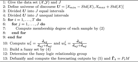
TABLE 3. The process of the HFs.

2.2.3 Machine Learning Technique

The methods based on machine learning have strong learning ability and can handle the non-linear components in the time series, so they have been widely used in some fields (Gündüz et al., 2019; Henrique et al., 2019; Volk et al., 2020; Wang et al., 2021b). In this study, three different networks were selected to analyze the series, since the features of the series are uncertain.

$(\mathcal{A})$ Back-Propagation Neural Network

Back-propagation neural network (BPnn) is a three-layer feed-forward network with an input layer, a hidden layer, and an output layer. Each layer takes inputs only from the previous layer and sends the outputs only to the next layer. Define the input vector as $\mathcal{X}=\{{\mathit{X}}_{\mathbf{1}},{\mathit{X}}_{\mathbf{2}},\dots ,{\mathit{X}}_{\mathit{N}}\}$, and the output vector as $\mathcal{Y}=\{{\mathit{Y}}_{\mathbf{1}},{\mathit{Y}}_{\mathbf{2}},\dots ,{\mathit{Y}}_{\mathit{N}}\}$. Assume the input layer has I neurons, the hidden layer has H neurons, and the output layer has one neuron, the network can be constructed as Figure 1B, and the training processes are described as follows.

FIGURE 1

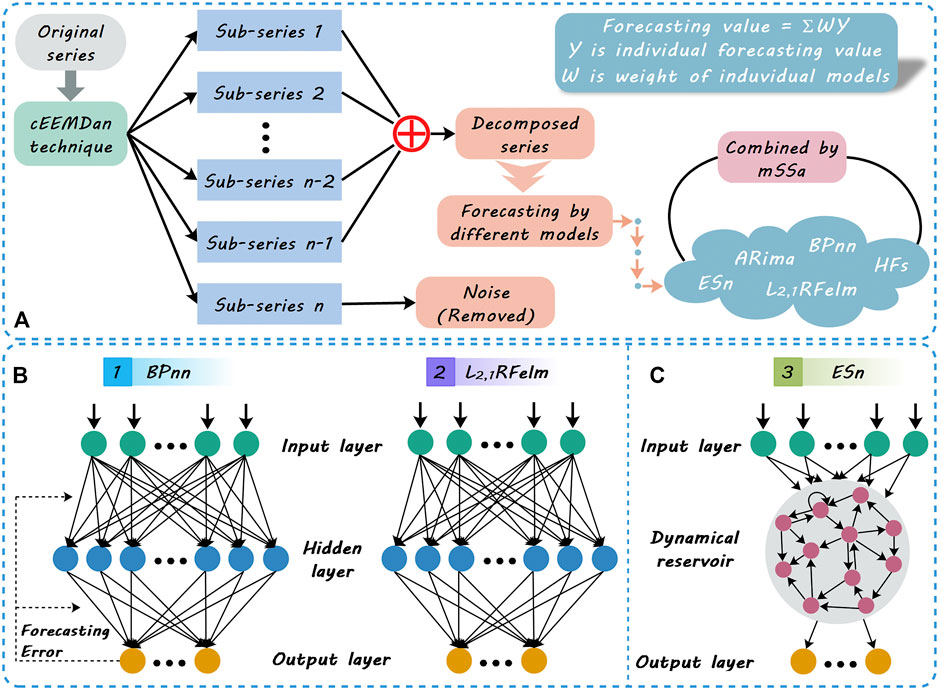
FIGURE 1. (A) is the flowchart of the proposed combined system; (B) and (C) are the structures of the neural networks used in this paper, where BPnn and ℓ_2,1RFelm have the same structure and different solution processes.

Calculate outputs of all neurons in hidden layer (Hecht-Nielsen, 1992; Wang Y. et al., 2021):

$\left\{\begin{array}{c}{\mathit{h}}_{\mathit{h}}^{\mathit{i}}={\sum }_{i=1}^I{w}_{ih}{x}_n+{\bar{\mathbf{\mho }}}_h,h=\mathrm{1,2},\dots ,H,\hfill \\ {\mathit{h}}_{\mathit{h}}^{\mathit{o}}=f({\mathit{h}}_{\mathit{h}}^{\mathit{i}}),h=\mathrm{1,2},\dots ,H,\hfill \end{array}\right.(6)$

Where, ${\mathit{h}}_{\mathit{h}}^{\mathit{i}}$ is the activation value of the h-th node of hidden layer, ${\mathit{h}}_{\mathit{h}}^{\mathit{o}}$ represents the output value of h-th hidden neuron, w_ih denotes the connection weight between i-th input neuron and h-th hidden neuron, ${\bar{\mathit{\mho }}}_h$ represents the bias of h-th hidden neuron, and f (⋅) is the activation function. Then, determine the output of the network as ${\mathit{O}}^{\mathit{o}}=g({\sum }_{h=1}^H{w}_h{\mathit{h}}_{\mathit{h}}^{\mathit{o}}+\overline{\stackrel{̄}{\mathit{\mho }}})$, where O^o is the output value of output neuron, w_h is the weight between h-th hidden neuron and output neuron, $\overline{\stackrel{̄}{\mathit{\mho }}}$ represents the bias of output neuron, and g (⋅) is the activation function. Obtain the minimum global error by the “error feedback” training mechanism. The global error is $\mathcal{E}={\sum }_{n=1}^N{({\mathit{O}}_{\mathit{n}}^{\mathit{o}}-{\mathit{Y}}_{\mathit{n}})}^2/2$, ${\mathit{O}}_{\mathit{n}}^{\mathit{o}}$ represents n-th output of network. For more details, please refer to (Hecht-Nielsen, 1992). For each iteration, the computational complexity of both the forward propagation process and the backward propagation process is $\mathcal{O}(N(H+1)(F+1)+N(H+1)(O+1))$, where F is the dimension of the input set and O represents the dimension of the output set. In this study, F = 4, O = 1, so the computational complexity of the algorithm is $T_{bpnn}\mathcal{O}(NH)$, here T_bpnn is the number of iterations.

$(\mathcal{B})$ ℓ_2,1-Norm and Random Fourier Mapping-Based Extreme Learning Machine

ℓ_2,1RFelm is an improved feed-forward neural network with a single hidden layer, which was proposed by Zhou et al. (2016). In this method, Random Fourier Mapping is used to improve the extendibility of the network by approximating the activation function in ELM. And ℓ_2,1-norm is used to make the hidden layer more compact and discriminative by cutting irrelevant neurons.

To predict the PM_2.5 concentration of the day, the PM_2.5 concentrations of the past 4 days are used. So, the original concentration series X = {x₁, x₂, … , x_T} is reconstructed as follows:

$\begin{array}{cc}\hfill \hfill & \hfill \mathcal{X}=[{\mathit{X}}_{\mathbf{1}},{\mathit{X}}_{\mathbf{2}},\dots ,{\mathit{X}}_{\mathit{N}}]=\left[\begin{array}{cccc}\hfill x_1\hfill & \hfill x_2\hfill & \hfill \cdots \hfill & \hfill x_{T-4}\hfill \\ \hfill x_2\hfill & \hfill x_3\hfill & \hfill \cdots \hfill & \hfill x_{T-3}\hfill \\ \hfill x_3\hfill & \hfill x_4\hfill & \hfill \cdots \hfill & \hfill x_{T-2}\hfill \\ \hfill x_4\hfill & \hfill x_5\hfill & \hfill \cdots \hfill & \hfill x_{T-1}\hfill \end{array}\right],\hfill \\ \hfill \hfill & \hfill \mathcal{Y}=[{\mathit{Y}}_{\mathbf{1}},{\mathit{Y}}_{\mathbf{2}},\dots ,{\mathit{Y}}_{\mathit{N}}]=[x_5,x_6,\dots ,x_{T-1},x_T].\hfill \end{array}(7)$

Then, the main processes of this method can be introduced as follows:

Randomly initialize the connection weights $\mathcal{W}$ between the input layer and hidden layer and the bias $\mathcal{B}$ of the hidden layer, assume the hidden layer has H neurons, these two matrix are represented as follows:

$\begin{array}{cc}\hfill \hfill & \hfill \mathcal{W}={\left[W_1,\dots ,W_h,\dots ,W_H\right]}^{\text{T}}=\left[\begin{array}{cccc}\hfill w_{11}\hfill & \hfill w_{12}\hfill & \hfill w_{13}\hfill & \hfill w_{14}\hfill \\ \hfill w_{21}\hfill & \hfill w_{22}\hfill & \hfill w_{23}\hfill & \hfill w_{24}\hfill \\ \hfill ⋮\hfill & \hfill ⋮\hfill & \hfill ⋮\hfill & \hfill ⋮\hfill \\ \hfill w_{H1}\hfill & \hfill w_{H2}\hfill & \hfill w_{H3}\hfill & \hfill w_{H4}\hfill \end{array}\right],\hfill \\ \hfill \hfill & \hfill \mathcal{B}=[b_1,\dots ,b_h,\dots ,b_H],h=\mathrm{1,2},\dots ,H,\hfill \end{array}(8)$

here w_H1 represents the weight between the first input neuron and H-th hidden neuron, b_h represents the bias of h-th hidden neuron. Then the output matrix of the hidden layer is

$\mathcal{H}=\left[\begin{array}{cccc}\hfill g(W_1{\mathit{X}}_{\mathbf{1}}+b_1)\hfill & \hfill g(W_1{\mathit{X}}_{\mathbf{2}}+b_1)\hfill & \hfill \cdots \hfill & \hfill g(W_1{\mathit{X}}_{\mathit{N}}+b_1)\hfill \\ \hfill g(W_2{\mathit{X}}_{\mathbf{1}}+b_2)\hfill & \hfill g(W_2{\mathit{X}}_{\mathbf{2}}+b_2)\hfill & \hfill \cdots \hfill & \hfill g(W_2{\mathit{X}}_{\mathit{N}}+b_2)\hfill \\ \hfill ⋮\hfill & \hfill ⋮\hfill & \hfill \ddots \hfill & \hfill ⋮\hfill \\ \hfill g(W_H{\mathit{X}}_{\mathbf{1}}+b_H)\hfill & \hfill g(W_H{\mathit{X}}_{\mathbf{2}}+b_H)\hfill & \hfill \cdots \hfill & \hfill g(W_H{\mathit{X}}_{\mathit{N}}+b_H)\hfill \end{array}\right].(9)$

In this method, the Random Fourier Mapping g (⋅) is used to approximate the kernel function, so $\mathcal{WX+B}$ can be mapped into a Random Fourier feature space. The specific mapping is defined as below (Rahimi and Recht, 2007):

$g(x)=\frac{1}{\sqrt{N}}{[\cos (w_1^{\text{T}}x),\dots ,\cos (w_N^{\text{T}}x),\sin (w_1^{\text{T}}x),\dots ,\sin (w_N^{\text{T}}x)]}^{\text{T}}.(10)$

Then, calculate the output of the network and solve parameter. Let the connection weight between the hidden layer and the output layer is $\mathit{\beta }={[{\beta }_1,{\beta }_2,\dots ,{\beta }_H]}^{\text{T}}$, then the output function of this network is ${\sum }_{h=1}^H{\beta }_{h}g(W_h{\mathit{X}}_{\mathit{n}}+{\bar{\mathit{\mho }}}_h)=O_i,n=\mathrm{1,2},\dots ,N$. In ℓ_2,1RFelm, the only parameter need to solve is β. Based on the given data and the initial parameters, the objective function of this network is

$\begin{array}{cc}\hfill \hfill & \hfill \underset{\mathit{\beta },\epsilon }{\mathrm{Min}}\frac{1}{2}\Vert \mathit{\beta }{\Vert }_{\mathrm{2,1}}+\frac{1}{2}\tilde{\text{C}}{\sum }_{i=1}^N\Vert {\mathrm{\Upsilon }}_i{\Vert }^2,\hfill \\ \hfill \hfill & \hfill \mathbf{s}.\mathbf{t}.g({\mathit{X}}_{\mathit{i}})\mathit{\beta }=y_i-{\mathrm{\Upsilon }}_i,i=\mathrm{1,2},\dots ,\text{N},\hfill \end{array}(11)$

chere ɛ represents the training error, $\tilde{\text{C}}$ is the penalty coefficient, and ‖β^T‖_2,1 is ℓ_2,1-norm of β, $\Vert \mathit{\beta }{\Vert }_{\mathrm{2,1}}=\sqrt{{\sum }_{h=1}^H{\beta }_h^2}$. Finally, β can be obtained $\widehat{\mathit{\beta }}={\left(\mathbf{D}/\tilde{\mathrm{C}}+{\mathcal{H}}^{\text{T}}\mathcal{H}\right)}^{-1}{\mathcal{H}}^{\text{T}}{\mathcal{Y}}^{\text{T}}$, where D is a diagonal matrix with D_hh = 1/(2‖β‖₂), and at the beginning of the iterative, D is an identity matrix. For more details of solve process, please refer to (Zhou et al., 2016). In this study, the computational complexity of ℓ_2,1RFelm is mainly contributed by the process of computing ${\left(\mathbf{D}/\tilde{\text{C}}+{\mathcal{H}}^{\text{T}}\mathcal{H}\right)}^{-1}$. Thus the computational complexity of ℓ_2,1RFelm is $T_{rfelm}\mathcal{O}(H^3)$, T_rfelm is the number of the iterations.

$(\mathcal{C})$ Echo State Network

Echo state network (ESn) is an improved recurrent neural network and was proposed in 2004 (Jaeger and Haas, 2004). Without output feedback connections, an ESn consists of an input layer with I neurons, L internal neurons possessing internal states, and one output neuron. The structure of ESn is shown in Figure 1C. Given a training set $[\mathcal{X},\mathcal{Y}]$ the main steps of ESn are as follows (Qiao et al., 2016; Wang et al., 2019). Randomly generate a reservoir weight matrix W with the predefined sparsity and size. In order for the reservoir to have echo-state property, the singular values of reservoir weight matrix of the reservoir must be scaled to within 1, so scaled W as $\tilde{\mathbf{W}}=(\mathbf{\alpha }/\mathbf{\Psi })\mathbf{W}$, here 0 < α < 1 and Ψ is the spectral radius of W. Next, randomly generate the weight matrix between input layer and reservoir, denoted as Wⁱⁿ. And initialize the reservoir states £ (0). Calculate the state of reservoir by using dynamic equation, £ (n+1) = $\mathcal{F}\left(\tilde{\mathit{W}}\right.$ £ (n)$\left.+{\mathit{W}}^{in}{\mathit{X}}_{\mathit{n}+\mathbf{1}}\right)$, here £ (n) and £ (n+1) are reservoir states, $\mathcal{F}(\cdot )$ is activation function, X_n+1 represent (n + 1)-th sample input. Finally, calculate the network output ${\widehat{y}}_{n+1}=\mathcal{G}\left({\mathit{W}}^{out}\right.$£ (n+1)), where W^out represents weight matrix between reservoir and output layer, $\mathcal{G}(\cdot )$ is activation function. The only trainable part of the ESn is the output weight matrix W^out, and can be commonly obtained as ${\mathit{W}}^{out}={\left({\mathcal{X}}^{\text{T}}\mathcal{X}\right)}^{-1}{\mathcal{X}}^{\text{T}}\mathcal{Y}$. As shown above, the computational complexity of ESn is largely proportional to the state updating process, the complexity of this process is equal to $\mathcal{O}(LT)$, where T is the number of sample.

2.3 Optimization of Combination Weights

Mirjalili et al. proposed a novel swarm intelligence optimization algorithm in 2017, which was inspired by the behavior of salps looking for food (Mirjalili et al., 2017a). Their study has shown that this method can approximate the Pareto optimal solution with high convergence and coverage. It has merits among the current optimization algorithms and is worth applying to different problems (Mirjalili et al., 2017a). Therefore, this method (mSSa) is used to find the optimal combined weight of different forecasting models in this study. More details are introduced as follows.

2.3.1 Multi-Objective Optimization

Multi-objective optimization is concerned with mathematical optimization problems involving more than one objective function to be optimized simultaneously (Haimes et al., 2011). The multi-objective optimization problem can represent as follows:

$\left\{\begin{array}{c}\text{Minimize}[{\mathbf{O}\mathbf{b}\mathbf{f}}_1(x),{\mathbf{O}\mathbf{b}\mathbf{f}}_2(x),\dots ,{\mathbf{O}\mathbf{b}\mathbf{f}}_o(x)],\hfill \\ \text{subject\hspace{0.17em}to}x\in \mathcal{S},\hfill \end{array}\right.(12)$

where $\mathcal{S}$ is the feasible search space, o is the number of objective function, and Obf_i is i-th objective function.

The purpose of multi-objective optimization is to find the set of acceptable solutions (Ngatchou et al., 2005). Hence, the definitions related to the Pareto-optimal solutions are introduced.

Definition 1. Pareto domination Given two vectors $\vec{\mathbf{X}}=(x_1,x_2,\dots ,x_n)$ and $\vec{\mathbf{Y}}=(y_1,y_2,\dots ,y_n)$, vector $\vec{\mathbf{Y}}$ dominates $\vec{\mathbf{X}}$ or called vector $\vec{\mathbf{X}}$ is dominated by vector $\vec{\mathbf{Y}}$ denoted as $\vec{\mathbf{Y}}\prec \vec{\mathbf{X}}$ if and only if $\forall i\in [1,o],\left[{\mathbf{O}\mathbf{b}\mathbf{f}}_i(\vec{\mathbf{Y}})\le {\mathbf{O}\mathbf{b}\mathbf{f}}_i(\vec{\mathbf{X}})\right]\wedge \exists i\in [1,o],\left[{\mathbf{O}\mathbf{b}\mathbf{f}}_i(\vec{\mathbf{Y}})<{\mathbf{O}\mathbf{b}\mathbf{f}}_i(\vec{\mathbf{X}})\right]$, where Obf_i (⋅) represents i-th objective function.

Definition 2. Pareto optimal set A set including all the non-dominated solutions is called Pareto optimal set. The mathematical description is ${\mathbf{P}}_s≔\left\{x,z\in \vec{\mathbf{X}}\mid \nexists z\prec x\right\}$.

2.3.2 Process of Multi-Objective Salp Swarm Algorithm

The individuals in a salp chain are divided into two groups: the front of the chain is the leader, the others are followers. Assume O indicates the dimension of search space, N denotes the number of salp chains, then the location of all the salps can be defined as a matrix:

${\mathcal{P}}_t=\left[\begin{array}{cccc}\hfill p_1^1(t)\hfill & \hfill p_2^1(t)\hfill & \hfill \dots \hfill & \hfill p_O^1(t)\hfill \\ \hfill p_1^2(t)\hfill & \hfill p_2^2(t)\hfill & \hfill \dots \hfill & \hfill p_O^2(t)\hfill \\ \hfill ⋮\hfill & \hfill ⋮\hfill & \hfill \dots \hfill & \hfill ⋮\hfill \\ \hfill p_1^N(t)\hfill & \hfill p_2^N(t)\hfill & \hfill \dots \hfill & \hfill p_O^N(t)\hfill \end{array}\right].(13)$

here t represents t-th iteration. The position of each salp is a candidate solution. Next, calculate fitness of each salp chain $\mathbf{F}\mathbf{i}\mathbf{t}[{\vec{p}}^j(t)]=\left\{ob{f}_1[{\vec{p}}^j(t)],ob{f}_2[{\vec{p}}^j(t)],\dots ,ob{f}_O[{\vec{p}}^j(t)]\right\},j=\mathrm{1,2},\dots ,N$, where $\mathbf{F}\mathbf{i}\mathbf{t}[{\vec{p}}^j(t)]$ represents the fitness of j-th salp chain at t-th iteration, $ob{f}_o[{\vec{p}}^j(t)]$ is the value of o-th objective function of j-th salp chain at t-th iteration. Then, determine the non-dominated salp chains according to Definition 1, and update the archive (Pareto optimal set, Definition 2). Select a salp chain as a food source from the archive, denoted as F. After that, leaders p₁ guides the salp swarm toward the food source in an O-dimensional search space. The positions of the leaders are updated as follows (Mirjalili et al., 2017a):

$p_1^i(t+1)=\left\{\begin{array}{cc}{\mathbf{F}}_i(t)+{\mathit{\tau }}_1\left[\left(\overline{\stackrel{̄}{p_1}}-{\underline{\underline{p}}}_1\right){\mathit{\tau }}_2+{\underline{\underline{p}}}_1\right],\hfill & {\mathit{\tau }}_3\ge 0,\hfill \\ {\mathbf{F}}_i(t)-{\mathit{\tau }}_1\left[\left(\overline{\stackrel{̄}{p_1}}-{\underline{\underline{p}}}_1\right){\mathit{\tau }}_2+{\underline{\underline{p}}}_1\right],\hfill & {\mathit{\tau }}_3<0,\hfill \end{array}\right.(14)$

where $p_1^i(t+1)$ is the position of leader in the i-th chain at (t + 1)-th iteration, F_i(t) represents the food source position in the i-th dimension at t-th iteration. ${\underline{\underline{p}}}_1$ and $\overline{\stackrel{̄}{p_1}}$ are the lower bound and the upper bound of p₁.

In Eq. 14, τ₁ is a parameter that controls the balance of exploration and exploitation, τ₂ is a random number in (0, 1) that determines the distance to move, and τ₃ is also a random number in (0, 1) that determines the direction of movement. The coefficient τ₁ is defined as ${\mathit{\tau }}_1=2e^{-{(4t/{\mathit{T}}_{\mathit{m}\mathit{S}\mathit{S}\mathit{a}})}^2}$, where t is the number of the current iteration and T_mSSa represents the number of maximum iteration. Whereafter, the positions of the followers are mathematically updated as $p_j^i(t+1)=\frac{1}{2}\left[p_j^i(t)+p_j^{i-1}(t)\right],\forall 2\le j,i=\mathrm{1,2},\dots ,N$. Finally, repeat the processes of calculating fitness, updating the archive, selecting food source and updating the salps location until satisfied with the end condition.

If the archive is not full, the non-dominated solutions are saved to the archive after comparison according to Definition 1, otherwise, before storage deletes some solutions (Mirjalili et al., 2017a). According to the principle of improving the distributivity of solutions in the archive, use the Roulette Wheel mechanism to remove the densest solutions. The probability of the solution being removed can be calculated as P_r = N_l/c, where N_l is the number of l-th solution in the archive, and c is a constant greater than 1 (Mirjalili et al., 2017b).

According to the introduction of mSSa, the computational complexity of this method is $\mathcal{O}(O\times N+cof\times N+2N^2)$ at one iteration, where cof is the computational complexity of the objective function. In this study, the Mean Square Error and the Standard deviation of the error are set as objective function. The complexity of the first objective functions is $\mathcal{O}(T^2)$ and the second objective function is $\mathcal{O}(T)$. Therefore, the complexity of one iteration of mSSa is $\mathcal{O}(O\times N+(T^2+T)\times N+2N^2)$, here T is the number of samples.

2.4 The Proposed Combined Forecasting System

Using the aforementioned methods and strategy, a novel combined pollutant concentration forecasting system based on the data decomposition strategy, several individual forecasting models, and a multi-objective optimization algorithm is designed.

Assume there are M models to predict the pollutant concentration, the forecasting results are denoted as ${\widehat{Y}}_m,(m=\mathrm{1,2},\dots ,M)$, and the weight coefficients of each forecasting result are ω₁, ω₂, … , ω_M, then the combined system can be expressed in mathematical form as

$\left\{\begin{array}{c}\mathbf{F}={\sum }_{m=1}^M{\omega }_m{\widehat{Y}}_m,\hfill \\ \sum _{m=1}^M{\mathrm{\Omega }}_m=1,\hfill \end{array}\right.(15)$

here F is the final forecasting result.

The main steps of this proposed system are listed as follows, and the flowchart of this study is described in Figure 1.

Pre-processing of original data. Since the original series are fluctuating, it is difficult to analyze its features. Therefore, the strategy of “decomposition and ensemble” is utilized to distinguish different characteristics and noise in the original series. And then, the noise is filtered out to reconstruct a more stable series. The parameters of this method are shown in Table 5.

Forecasting by individual models. Since the features hidden in the series are not certain, three types of methods were used to analyze the series and implement forecasting. These methods contain a traditional statistical model (ARima), a hesitant fuzzy time series forecasting model, and machine learning models (BPnn, ℓ_2,1RFelm, ESn). In the three machine learning models, BPnn and ℓ_2,1RFelm have the same network structure but different solving strategies, BPnn and ESn have different network structures but the same solving strategy, and ℓ_2,1RFelm and ESn have different network structures and solving strategies.

Construction of the combined system. In order to obtain more accurate forecasting results, use mSSa to conduce the optimal combined weights of the individual models. More specifically, take the predicted values obtained by each individual model as input and the true concentration values as output to form a training set. Then, the optimization algorithm is trained based on this set and finally obtains the optimal weight vector. Afterward, the forecasting results of such individual models are combined together by using optimal weight to obtain the final forecasting value.

3 Empirical Analysis

In this study, the concentration of PM_2.5 is forecast by the proposed combined system. This section mainly introduces the experimental process and analyzes the forecasting results.

3.1 Data Description

Three PM_2.5 concentration data sets collected from the Pearl River Delta (PRD) region in China are selected as illustrative examples to verify the effectiveness of the proposed combined prediction system, including Guangzhou (GZ), Shenzhen (SZ), and Zhuhai (ZH). There are few missing data in these series, and the moving median method with a window length of 10 is used to fill in the missing data. Some statistical indicators for these three data sets are presented in Table 4. Considering the availability of data, the hourly concentrations were collected from 2020.04.29 to 2020.09.25, and these data were divided twice. In the forecasting module, the original data sets were divided into training sets and test sets, and the train to test ratio of each study city is   Tr₁:Te₁ = 7 : 3. And in the combination module, Te₁ was divided into training set   Tr₂ and test set Te₂, the division ratio is 7:3.

TABLE 4

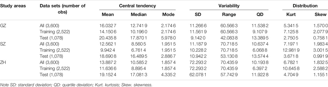
TABLE 4. Descriptive statistics of data sets.

3.2 Evaluation Metrics

In previous studies, numerous metrics have been utilized to evaluate model performance. To scientifically assess the proposed system, three metrics are selected as evaluation criteria, including two scale-dependent indicators and a percentage indicator. Details are as follows.

3.2.1 Scale-dependent Indicators

The unit of this type of indicator is the same as the unit of original data, so it can not be used to compare two series with different units. Two commonly used scale-dependent measures are Mean absolute error and Root mean squared error, they are based on absolute errors and squared errors, respectively (Hyndman and Athanasopoulos, 2018).

$\mathcal{A}$. Mean Absolute Error

The mean absolute error (MAE) is a commonly used indicator to evaluate the deviation between forecast values and true values (Khair et al., 2017):

$\mathbf{M}\mathbf{A}\mathbf{E}=\frac{1}{N}\sum _{n-1}^N|A_n-F_n|,(16)$

where N is the sample size, A_n represents the actual value of n-th sample, and F_n indicates the n-th forecast value. This metric can avoid the cancellation of the positive and negative predicted errors. The lower the value of MAE, the better the model is. MAE = 0 indicates that there is no error in the forecasting.

$\mathcal{B}$. Root Mean Squared Error

The root mean squared error (RMSE) is a commonly used measure of the forecasting results of machine learning models. Its equation is shown in (Eq. 17) (Wang Y. et al., 2021)

$\mathbf{R}\mathbf{M}\mathbf{S}\mathbf{E}=\sqrt{\frac{1}{N}\sum _{n=1}^N{(A_n-F_n)}^2}.(17)$

Same to the MAE, the lower the value of RMSE, the better the prediction. But RMSE is more sensitive to extreme values. Therefore, if the difference between RMSE and MAE is large, the greater the possibility of large errors existing in forecasting.

3.2.2 Percentage Indicator

The frequently used percentage indicator is the mean absolute percentage error (MAPE). It is often used in practice since it is a very intuitive explanation in terms of relative error and is unit-free. Its equation is shown as follows (Khair et al., 2017):

$\mathbf{M}\mathbf{A}\mathbf{P}\mathbf{E}=\frac{1}{N}\sum _{n=1}^N\left|\right.\frac{A_n-F_n}{A_n}\left|\right.\times 100\%.(18)$

Compared to MAE, this indicator is normalized by actual value, and useful when the size or size of a prediction variable is significant in evaluating the accuracy of forecasting (Khair et al., 2017). However, when there is 0 in the actual value, this indicator can not be used. MAPE = 0% indicates a perfect model, while MAPE = 100% indicates a poor model.

3.3 Parameter Settings

Different parameters of the model will lead to different results, so the analysis of the predicted results should be based on the parameters used. The model parameters used in this paper are shown in Table 5. For ARima, the optimal lag order, the optimal degree of difference, and the optimal order of the moving average are determined based on the Akaike Information Criterion (AIC). And all the empirical experiments are implemented on MATLAB R2020a, run on the Windows 10 professional operating system.

TABLE 5

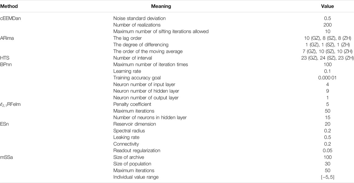
TABLE 5. Experimental parameter settings of different individual models.

3.4 Experiments and Results Analysis

In this study, three comparisons are implemented based on the data from GZ, SZ, and ZH in China. The first comparison is implemented to verify the effectiveness of the data decomposition strategy, the second comparison compares the different combination methods, and the last comparison compares the individual forecasting methods with the combined forecasting system. The forecasting performance lists in Table 6 and the specific results are analyzed as follows.

TABLE 6

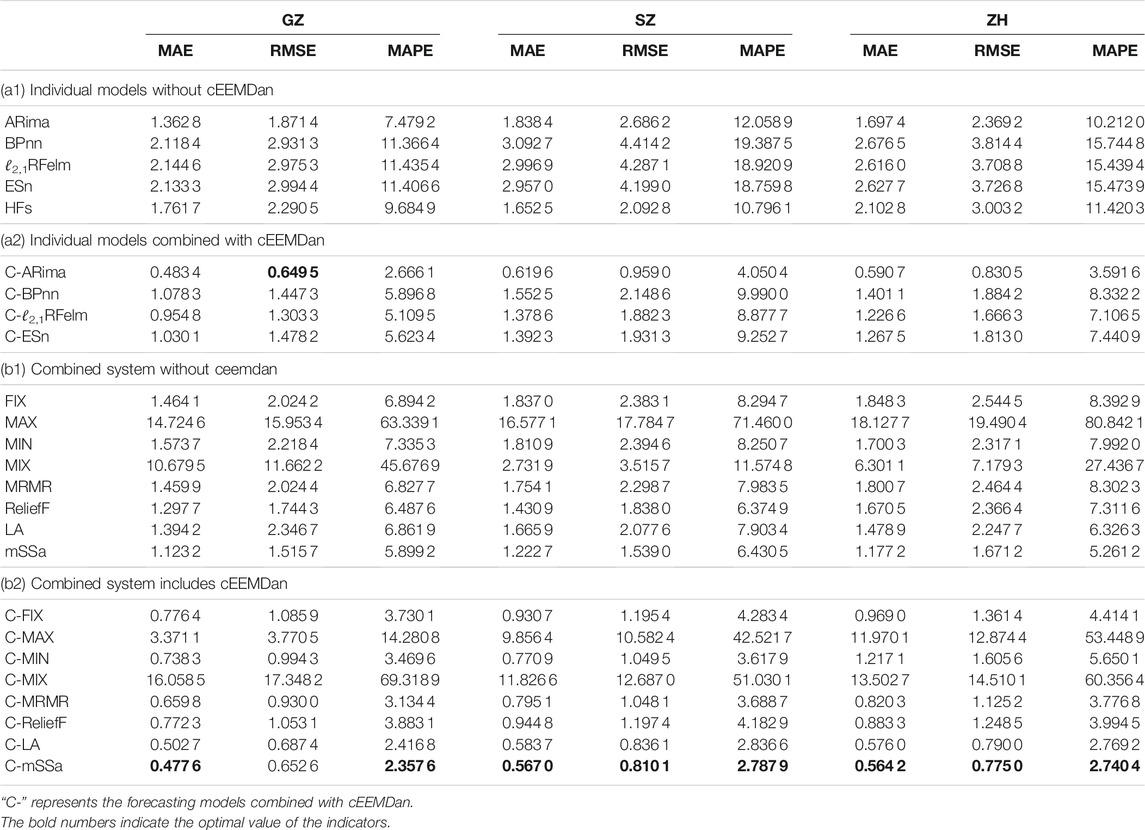
TABLE 6. Forecasting results of individual models and combined systems based on the original data and decomposed data.

3.4.1 Comparison I

This comparison is set to compare the forecasting accuracy between the models combining the cEEMDan and models without combining cEEMDan. The comparisons are divided into two categories, one for individual models and one for the combined system. The first category contains comparisons of ARiam vs. C-ARima, BPnn vs. C-BPnn, ℓ_2,1RFelm vs. C-ℓ_2,1RFelm, and ESn vs. C-ESn. Here, the hesitant fuzzy time series forecasting method has fuzzed the original series and constructed a transition matrix based on the fuzzy logic relationship group to forecast pollution concentration. These operations have compressed and filtered the information of the original series, so the hesitant fuzzy time series forecasting experiment based on the composed data is no longer carried out. The second category contains comparisons of FIX vs. C-FIX, MAX vs. C-MAX, MIN vs. C-MIN, MRMR vs. C-MRMR, ReliefF vs. C-ReliefF, LA vs. C-LA, and mSSa vs. C-mSSa.

1) From the results in Table 6 (a1) and (a2), it can be found that the forecasts based on the decomposed data are more accurate than based on the original data. Take the results from Guangzhou as an example. The maximum MAPE of the forecasts based on decomposed data (${\mathrm{M}\mathrm{A}\mathrm{P}\mathrm{E}}_{GZ}^{C-BPnn}$ = 5.896 8%) is lower than the minimum MAPE of the forecasts based on the original data (${\mathrm{M}\mathrm{A}\mathrm{P}\mathrm{E}}_{GZ}^{ARima}$ = 7.479 2%). And the MAE values of the forecasts based on the original data are all greater than 1.1 (MAE_GZ > 1.1), but the MAE values of the forecasts based on the decomposed data are all less than 1.1 (${\mathrm{M}\mathrm{A}\mathrm{E}}_{GZ}^C<$1.1), especially the (${\mathrm{M}\mathrm{A}\mathrm{E}}_{GZ}^{C-ARima}<$0.5), which is the best performance among all the forecasting models. The value of RMSE also shows the same result. The values of RMSE for the forecasts based on the original data are all greater than the values of RMSE for the forecasts based on the decomposed data (${\mathrm{R}\mathrm{M}\mathrm{S}\mathrm{E}}_{GZ}>{\mathrm{R}\mathrm{M}\mathrm{S}\mathrm{E}}_{GZ}^C$), which indicates that the forecasting values based on the decomposed data are closer to the true values. The sub-figures in Figure 2 show the predicted results of these models.

2) The strategy of “decomposition and ensemble” to remove noise contributes to improving the forecasting accuracy. The figures in Table 6 (b1) and (b2) show the forecasting results of combined systems. Take ZH as an example, the values of the indicators of the mSSa combination method are (1.177 2, 1.671 2, 5.261 2%)_{MAE, RMSE, MAPE}. But, the results obtained by the proposed cEEMDan-mSSa based method are (0.564 2, 0.775 0, 2.740 4%)_MAE, _RMSE, _MAPE, these three values are lower compared to the index results of mSSa based combined method. The same relationship can be found in the indicator results for GZ and SZ.

FIGURE 2

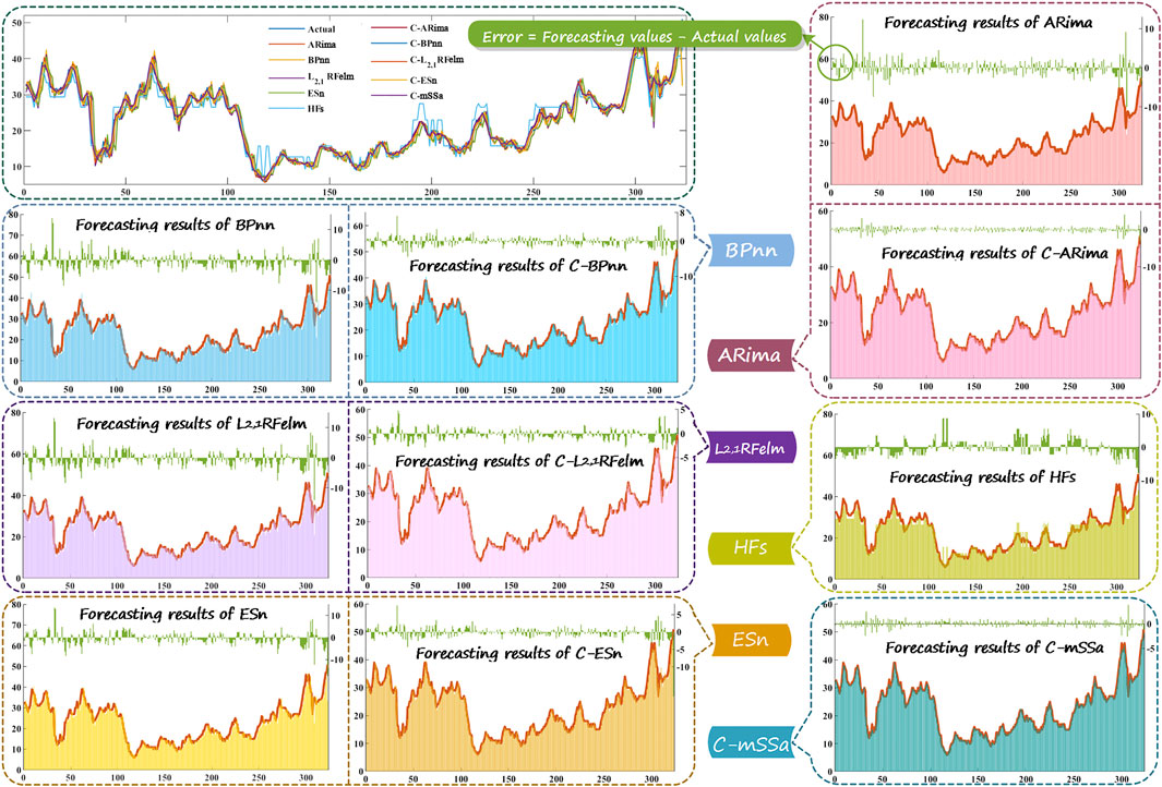
FIGURE 2. The forecasting results of the different models, where “C-” represents the forecasting models combined with cEEMDan.

Then, by comparing the remaining figures, it can be found that the values of indicators for systems without combining data decomposition strategy are smaller than the values of combining data decomposition strategy except for the MIX combined method. Take GZ as an example, all the values of MAE are greater than 1 of the method without combining cEEMDan (MAE_GZ > 1), but the values of these indicators are less than 1 for the method combining cEEMDan except for MAX and MIX combined methods (${\mathbf{M}\mathbf{A}\mathbf{E}}_{GZ}^C<$1). So as the values of RMSE and MAPE, the figures for the methods without combining cEEMDan are greater than the figures for methods combining cEEMDan. Therefore, it can be considered that no matter which combination method, the forecasting based on the decomposed data is more accurate.

Remark: Through the comparisons between the models combining the cEEMDan and models without combining cEEMDan, what can be found is that the data decomposition strategy can effectively improve the prediction ability of the model.

3.4.2 Comparison II

This comparison is set to compare the combination methods. These methods contain four numerical methods (FIX¹, MAX², MIN³, MIX⁴), two feature selection methods (MRMR, ReliefF), and two optimization algorithms, the Lichtenberg algorithm (LA) and mSSa. The results in Table 6 (b1) and (b2), and Figure 3 demonstrate that after data decomposition, the forecasting accuracy is improved. Moreover, the proposed combined model performance is best. The detailed analyses are as follows.

1) The multi-objective optimization method is the best weighting method. For the results in Table 6 (b1), it can be seen that the indicators’ values of mSSa are the smallest. Take GZ as an example, the indicators’ values of mSSa are (1.123 2, 1.515 7, 5.899 2%)_MAE, _RMSE, _MAPE, the minimum indicators’ values of the numerical methods are ${\mathrm{M}\mathrm{A}\mathrm{E}}_{GZ}^{FIX}$ = 1.464 1, ${\mathrm{R}\mathrm{M}\mathrm{S}\mathrm{E}}_{GZ}^{FIX}$ = 2.024 2, ${\mathrm{M}\mathrm{A}\mathrm{P}\mathrm{E}}_{GZ}^{FIX}$ = 6.894 2, and the minimum indicators’ values of the feature selected methods are ${\mathrm{M}\mathrm{A}\mathrm{E}}_{GZ}^{ReliefF}$ = 1.297 7, ${\mathrm{R}\mathrm{M}\mathrm{S}\mathrm{E}}_{GZ}^{ReliefF}$ = 1.744 3, ${\mathrm{M}\mathrm{A}\mathrm{P}\mathrm{E}}_{GZ}^{ReliefF}$ = 6.487 6. Based on these indicators’ values, it can be seen that the mSSa method has the best forecasting results. So as the results in SZ and ZH, the indicators’ values obtained by mSSa method are smaller than the value of other methods.

2) Check the results in Table 6 (b2), take SZ as an example, the MAE of numerical methods are (0.9307, 9.8564,0.7709, 11.8266)_FIX, _MAX, _MIN, _MIX, MAE of feature selected methods are (0.7951, 0.9448)_MRMR, _ReliefF, and for the optimization methods are (0.5837, 0.5670)_LA, _mSSa. And min(MAE) ${=\mathbf{M}\mathbf{A}\mathbf{E}}_{SZ}^{C-mSSa}$ = 0.5670. The same result can be obtained in GZ and ZH. Based on the results shown in the tables, it can be considered that the mSSa optimization algorithm is optimal as a weighting method.

3) The forecasts of the proposed combined system are more accurate than the mSSa based system. As the forecasting results shown in Table 6 (b1) and (b2), the MAE values of the proposed combined system in the three study cities are MAE^C−mSSa = (0.477 6, 0.567 0, 0.564 2)_GZ,SZ,ZH, these values are less than 0.6, but the MAE values of the system based on the original data are greater than 1.1 for three study cites (MAE^mSSa = (1.123 2, 1.222 7, 1.177 2)_GZ,SZ,ZH). Moreover, the MAPE values of the proposed system are MAPE^C−mSSa = (2.357 6%, 2.787 9%, 2.740 4%)_GZ,SZ,ZH, compared to the mSSa-based system they are improved by (60.04, 56.65, 47.91%)_GZ,SZ,ZH⁵. Since the smaller the values of the three metrics, the better the forecasting. Therefore, the results of these metrics indicate that the proposed combined system is performing better than the other system. The same conclusion can be drawn from the values of RMSE.

FIGURE 3

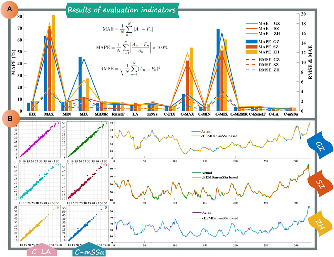
FIGURE 3. The forecasting results of the different combined methods. (A) is the results of evaluation indicators of three study cities. (B) is the forecasting results of C-LA and C-mSSa, where “C-” represents the cEEMDan.

Remark: The optimization algorithm combination methods are performing better than the other combination methods, especially better than the numerical combination methods. The weights determined by the numerical methods only consider part of the samples, so when the data fluctuates greatly, this type of method cannot get good forecasting results. And the weights determined by the feature selection methods and the optimization algorithms consider all the samples, including samples with large fluctuations, so the impact of large fluctuations can be reduced during the forecasting process.

3.4.3 Comparison III

This experiment compares the forecasting performance of the individual forecasting models and the combined forecasting system. The proposed forecasting system performs better than the individual forecasting models. Almost all the indicators’ values in the Table 6 (b1) and (b2) are smaller than those in the Table 6 (a1) and (a2), except for the MAX combination method and MIX combination method. Based on the data of SZ, the min(MAPE_SZ) ${=\mathbf{M}\mathbf{A}\mathbf{P}\mathbf{E}}_{SZ}^{C-ARima}$ = 4.0504, but this value is still greater than the ${\mathrm{M}\mathrm{A}\mathrm{P}\mathrm{E}}_{SZ}^{C-mSSa}$ = 2.7879%. The results of the other two metrics of SZ also show the same relationship. The min(MAE_SZ) and min(RMSE_SZ) are (0.5670, 0.8101), and all are obtained by the proposed forecasting system. These results indicate that the proposed combined forecasting system outperforms the individual forecasting models. The metric results of ZH can also draw the same conclusion as SZ. The results in GZ are a little different. The min(RMSE_GZ) = ${\mathrm{R}\mathrm{M}\mathrm{S}\mathrm{E}}_{GZ}^{C-ARima}$ = 0.649 5, and ${\mathrm{R}\mathrm{M}\mathrm{S}\mathrm{E}}_{GZ}^{C-mSSa}$ = 0.652 6, which is only 0.0031 different from the result of C-ARima. Therefore, the performance of the combined forecasting system can be regarded as better than the performance of the individual models.

In summary, the following conclusions can be drawn. The data decomposition strategy can significantly improve forecasting accuracy. These experimental results show that the forecasting results of all methods combined with cEEMDan, except MIX, are more accurate than the methods not combined with cEEMDan. In addition, the mSSa method has the best forecasting results among these combined methods, thus proving the forecasting performance of the proposed system is best.

Remark: For forecasting, data preprocessing is important. In this study, a powerful data decomposition strategy was used to decompose the original data series, and then discarded the noise component of the series. This processing improves the accuracy of the forecasting, and this conclusion is reached in two experiments. For combination, the multi-objective optimization method works better, and the numerical methods are the worst, and the performance is unstable. When the results of other methods become better, the numerical method performs worse.

4 Test of Forecasting System

In order to verify the significance and stability of the proposed forecasting system, the Diebold-Mariano test (DM) (Francis and Roberto, 1995) and the variance ratio (VR) are introduced in this study. The related details and results are described in this section.

4.1 Diebold-Mariano Test

DM is a hypothesis testing method to analyze the difference in prediction accuracy. According to the constructed DM statistics, it can be judged whether the difference of the prediction method is significant. In this test, the null hypothesis (H₀) and the alternative hypothesis (H₁) are as follows:

$\begin{array}{c}\hfill {\mathit{H}}_{\mathbf{0}}:\overline{\stackrel{̄}{\mathit{E}}}[\tilde{\mathcal{L}}({\breve{\mathit{\delta }}}_{\mathbf{1}}^{\mathit{t}})]=\overline{\stackrel{̄}{\mathit{E}}}[\tilde{\mathcal{L}}({\breve{\mathit{\delta }}}_{\mathbf{2}}^{\mathit{t}})]\hfill \\ \hfill {\mathit{H}}_{\mathbf{1}}:\overline{\stackrel{̄}{\mathit{E}}}[\tilde{\mathcal{L}}({\breve{\mathit{\delta }}}_{\mathbf{1}}^{\mathit{t}})]\ne \overline{\stackrel{̄}{\mathit{E}}}[\tilde{\mathcal{L}}({\breve{\mathit{\delta }}}_{\mathbf{2}}^{\mathit{t}})]\hfill \end{array}(19)$

here ${\breve{\mathit{\delta }}}_{\mathbf{1}}^{\mathit{t}}$ and ${\breve{\mathit{\delta }}}_{\mathbf{2}}^{\mathit{t}}$ represent the forecasting errors of forecasting model 1 and forecasting model 2 at t-th, $\tilde{\mathcal{L}}(\cdot )$ represents the loss function. Then, the DM statistic is constructed as follows (Huang et al., 2021):

$\mathbf{D}\mathbf{M}=\frac{{\sum }_{\mathit{t}=\mathbf{1}}^{\mathit{n}}[\tilde{\mathcal{L}}({\breve{\mathit{\delta }}}_{\mathbf{1}}^{\mathit{t}})-\tilde{\mathcal{L}}({\breve{\mathit{\delta }}}_{\mathbf{2}}^{\mathit{t}})]/\mathit{n}}{\sqrt{{\mathit{S}}^{\mathbf{2}}/\mathit{n}}}(20)$

where S² denotes the variance estimation of ${\breve{\mathit{\delta }}}_{\mathbf{1}}^{\mathit{t}}-{\breve{\mathit{\delta }}}_{\mathbf{2}}^{\mathit{t}}$.

Given a certain significance level α, the critical value Z_α/2 can get, if the absolute value of DM statistic is greater than the Z_α/2, the null hypothesis H₀ is rejected, and the result that two forecasting methods have significant differences.

Table 7 gives the DM test results of different forecasting models. This study compares 24 forecasting models or systems with the proposed system. Compared with the forecasting model without cEEMDan, the proposed forecasting system is significantly better, since the values of DM statistic are greater than the critical value of 1% significance level. After combined with cEEMDan, the forecasting ability of individual forecasting models has been improved, but the DM test results show that their predictive ability is still inferior to the proposed forecasting system, since the lowest value of DM test is between the critical value of 10% significance level and the critical value of 15% significance level. The DM values of Table 7 (b) also show that the proposed forecasting system is significantly superior than the other combined forecasting system, especially the system without data decomposition strategy.

TABLE 7

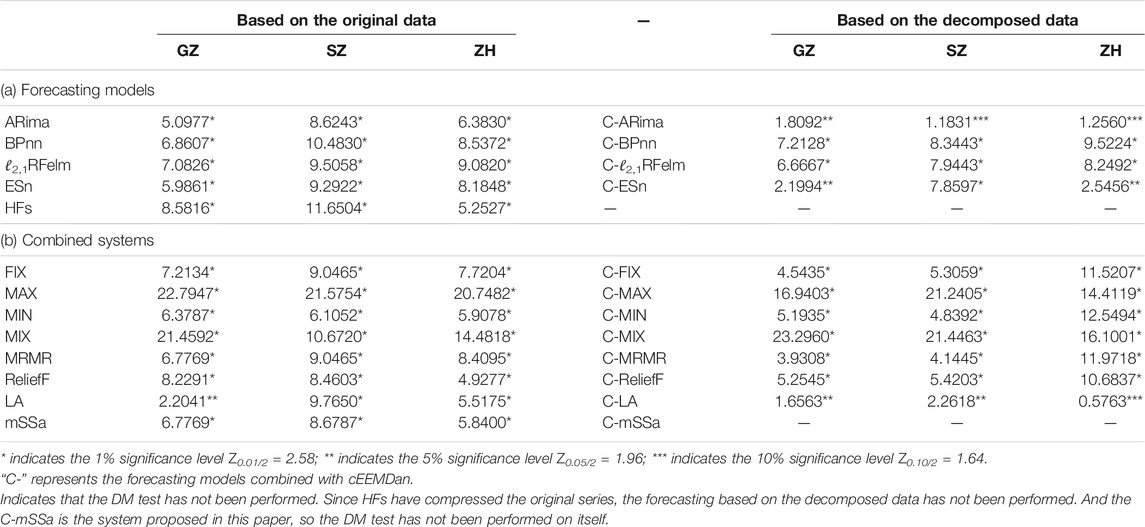
TABLE 7. DM test results of different models.

4.1.1 Stability Test

In order to validate the stability of models, the variance ratio (Vr) is introduced. Vr combines the variances of the forecasting value and the true value to illustrate the stability of the forecasting model. The greater the value of Vr, the higher the forecasting stability of the method (Huang et al., 2021).

$\mathit{V}\mathit{r}=\mathit{min}(\mathit{V}\mathit{a}{\mathit{r}}_{\mathit{f}\mathit{o}\mathit{r}\mathit{e}\mathit{c}\mathit{a}\mathit{s}\mathit{t}\mathit{i}\mathit{n}\mathit{g}}/\mathit{V}\mathit{a}{\mathit{r}}_{\mathit{a}\mathit{c}\mathit{t}\mathit{u}\mathit{a}\mathit{l}},\mathit{V}\mathit{a}{\mathit{r}}_{\mathit{a}\mathit{c}\mathit{t}\mathit{u}\mathit{a}\mathit{l}}/\mathit{V}\mathit{a}{\mathit{r}}_{\mathit{f}\mathit{o}\mathit{r}\mathit{e}\mathit{c}\mathit{a}\mathit{s}\mathit{t}\mathit{i}\mathit{n}\mathit{g}}),(21)$

here, Var_forecasting and Var_actual are the variances of the forecasting values and actual values.

The Vr results are shown in Table 8. The Vr values of the proposed system in the three cities are (0.986 1, 0.998 6, 0.985 9)_GZ,SZ,ZH. Although the Vr values of the proposed system are not the largest among all forecasting models and systems, these three values are all greater than 0.98, while the Vr values of most other forecasting models and systems are less than 0.98, indicating that the proposed forecasting system is relatively stable. Combined with the results of the forecasting evaluation metric shown in section 3, it shows that the proposed forecasting system has high prediction accuracy and relatively high stability.

TABLE 8

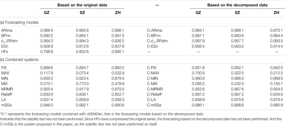
TABLE 8. Results of the model stability test.

5 Conclusion

Based on the multi-objective optimization algorithm and data decomposition strategy, an effective combined forecasting system is proposed to forecast the PM_2.5 concentration from Guangzhou, Shenzhen, and Zhuhai in China. The proposed system mainly contains three modules, the data preprocessing module, the individual model forecasting module, and the combination forecasting module. In the first module, the strategy of “decomposition and ensemble” is applied to remove the noise in the original series. In the individual model forecasting module, ARima, BPnn, ℓ_2,1RFelm, ESn, and HFs are applied to forecast PM_2.5 concentration respectively. These five models are from different kinds of forecasting models and are used to analyze different features in the PM_2.5 concentration series. ARima is a classical traditional statistical forecasting method; BPnn, ℓ_2,1RFelm, and ESn are neural networks with different characteristics; hesitant fuzzy time series model is a fuzzy-based forecasting model. By comparing eight weighting methods from three categories, the best combination method is found as a multi-objective optimization weighting method.

The developed combined forecasting system has been successfully applied in PM_2.5 concentration forecasting. Based on the forecasting evaluation indicators, the forecasting performance of the proposed system is validated. Specifically, compared the models forecasting results based on data before and after the preprocessing of cEEMDan in Comparison I. In Comparison II, compare the system employing diverse combination methods. Compere between the individual models and the combined models in Comparison III. After these comparative experiments, it can be observed that the MAE and MAPE values of the proposed system are always lower than the values of individual models and other combination methods. For RMSE in Guangzhou, the value of the proposed system is slightly higher than the minimum RMSE value, but overall, the forecasting performance of the proposed system is still the best. Therefore, the proposed combined forecasting system, which combines different types of individual forecasting models, has high practical application potential in air pollution concentration forecasting.

Data Availability Statement

Publicly available datasets were analyzed in this study. This data can be found here: http://www.mep.gov.cn/.

Author Contributions

LB: Conceptualization, Methodology, Software, Writing-Original draft preparation. HL: Conceptualization, Software, Validation. BZ: Conceptualization, Supervision, Writing-Reviewing and Editing. XH: Conceptualization, Writing—Review and Editing, Data curation.

Funding

This work was supported by Major Program of National Social Science Foundation of China (Grant No. 17ZDA093).

Conflict of Interest

The authors declare that the research was conducted in the absence of any commercial or financial relationships that could be construed as a potential conflict of interest.

Publisher’s Note

All claims expressed in this article are solely those of the authors and do not necessarily represent those of their affiliated organizations, or those of the publisher, the editors and the reviewers. Any product that may be evaluated in this article, or claim that may be made by its manufacturer, is not guaranteed or endorsed by the publisher.

Footnotes

¹FIX represents a weighting method with fixed weights, and the weight of each forecasting model is 0.2.

²MAX represents the method of using the maximum forecasting error to assign weights, and the weight of each forecasting model is the reciprocal of the maximum forecasting error obtained by each model in the training set.

³MIN is opposite to MAX, using the minimum value of the forecasting error is used as the basis for weighting, the weight of wach methode is caluculated as $w_i=e_i/{\sum }_{i=1}^5{e}_i,e_i=1/m{e}_i,i=1,\dots ,5$, where me_i represents minimum error of i-th model.

⁴For MIX weighting method, the weight of each model is obtained by following equation: w_i = mean(|e_in|/A_n), i = 1, … , 5; n = 1.⋯ , N, here the e_in is forecasting errors of i-th model, A_n is the actual value of PM_2.5 concentration.

⁵The improved percentage is calculated as follows: ${\mathbf{P}}_{metric}=(V_m^{Model1}-V_m^{Model2})/V_m^{Model1}$. Such as the improved percentage of GZ’s MAPE is ((5.899 2–2.357 6)/5.899 2) × 100%.

References

Ariyo, A. A., Adewumi, A. O., and Ayo, C. K. (2014). “Stock price Prediction Using the Arima Model,” in 2014 UKSim-AMSS 16th International Conference on Computer Modelling and Simulation (Cambridge, UK: IEEE), 106–112. doi:10.1109/uksim.2014.67

CrossRef Full Text | Google Scholar

Benvenuto, D., Giovanetti, M., Vassallo, L., Angeletti, S., and Ciccozzi, M. (2020). Application of the Arima Model on the Covid-2019 Epidemic Dataset. Data in brief 29, 105340. doi:10.1016/j.dib.2020.105340

PubMed Abstract | CrossRef Full Text | Google Scholar

Bisht, K., and Kumar, S. (2016). Fuzzy Time Series Forecasting Method Based on Hesitant Fuzzy Sets. Expert Syst. Appl. 64, 557–568. doi:10.1016/j.eswa.2016.07.044

CrossRef Full Text | Google Scholar

Cheng, S.-H., Chen, S.-M., and Jian, W.-S. (2016). Fuzzy Time Series Forecasting Based on Fuzzy Logical Relationships and Similarity Measures. Inf. Sci. 327, 272–287. doi:10.1016/j.ins.2015.08.024

CrossRef Full Text | Google Scholar

Cheng, X., Liu, Y., Xu, X., You, W., Zang, Z., Gao, L., et al. (2019). Lidar Data Assimilation Method Based on Crtm and Wrf-Chem Models and its Application in pm2.5 Forecasts in Beijing. Sci. Total Environ. 682, 541–552. doi:10.1016/j.scitotenv.2019.05.186

PubMed Abstract | CrossRef Full Text | Google Scholar

Dėdelė, A., and Miškinytė, A. (2019). Seasonal and Site-specific Variation in Particulate Matter Pollution in lithuania. Atmos. Pollut. Res. 10, 768–775. doi:10.1016/j.apr.2018.12.004

CrossRef Full Text | Google Scholar

Francis, X., and Roberto, S. (1995). Comparing Predictive Accuracy. J. Business Econ. Stat. 13, 134. doi:10.1080/07350015.1995.10524599

CrossRef Full Text | Google Scholar

Gavirangaswamy, V. B., Gupta, G., Gupta, A., and Agrawal, R. (2013). “Assessment of Arima-Based Prediction Techniques for Road-Traffic Volume,” in Proceedings of the fifth international conference on management of emergent digital EcoSystems, 246–251. doi:10.1145/2536146.2536176

CrossRef Full Text | Google Scholar

Glencross, D. A., Ho, T.-R., Camiña, N., Hawrylowicz, C. M., and Pfeffer, P. E. (2020). Air Pollution and its Effects on the Immune System. Free Radic. Biol. Med. 151, 56–68. doi:10.1016/j.freeradbiomed.2020.01.179

PubMed Abstract | CrossRef Full Text | Google Scholar

Goyal, P., Chan, A. T., and Jaiswal, N. (2006). Statistical Models for the Prediction of Respirable Suspended Particulate Matter in Urban Cities. Atmos. Environ. 40, 2068–2077. doi:10.1016/j.atmosenv.2005.11.041

CrossRef Full Text | Google Scholar

Grennfelt, P., Engleryd, A., Forsius, M., Hov, Ø., Rodhe, H., and Cowling, E. (2020). Acid Rain and Air Pollution: 50 Years of Progress in Environmental Science and Policy. Ambio 49, 849–864. doi:10.1007/s13280-019-01244-4

PubMed Abstract | CrossRef Full Text | Google Scholar

Gündüz, D., de Kerret, P., Sidiropoulos, N. D., Gesbert, D., Murthy, C. R., and van der Schaar, M. (2019). Machine Learning in the Air. IEEE J. Selected Areas Commun. 37, 2184–2199.

CrossRef Full Text | Google Scholar

Haimes, Y. Y., Hall, W. A., and Freedman, H. T. (2011). Multiobjective Optimization in Water Resources Systems: The Surrogate worth Trade-Off Method. Amsterdam, Netherlands: Elsevier.

Google Scholar

Hecht-Nielsen, R. (1992). “Theory of the Backpropagation Neural Network**Based on "nonindent" by Robert Hecht-Nielsen, Which Appeared in Proceedings of the International Joint Conference on Neural Networks 1, 593-611, June 1989. 1989 IEEE,” in Neural Networks for Perception (Amsterdam, Netherlands: Elsevier), 65–93. doi:10.1016/b978-0-12-741252-8.50010-8

CrossRef Full Text | Google Scholar

Henrique, B. M., Sobreiro, V. A., and Kimura, H. (2019). Literature Review: Machine Learning Techniques Applied to Financial Market Prediction. Expert Syst. Appl. 124, 226–251. doi:10.1016/j.eswa.2019.01.012

CrossRef Full Text | Google Scholar

Huang, X., Wang, J., and Huang, B. (2021). Two Novel Hybrid Linear and Nonlinear Models for Wind Speed Forecasting. Energ. Convers. Manage. 238, 114162. doi:10.1016/j.enconman.2021.114162

CrossRef Full Text | Google Scholar

Hyndman, R. J., and Athanasopoulos, G. (2018). Forecasting: Principles and Practice. Melbourne, Australia: OTexts.

Google Scholar

Jaeger, H., and Haas, H. (2004). Harnessing Nonlinearity: Predicting Chaotic Systems and Saving Energy in Wireless Communication. science 304, 78–80. doi:10.1126/science.1091277

PubMed Abstract | CrossRef Full Text | Google Scholar

Khair, U., Fahmi, H., Hakim, S. A., and Rahim, R. (2017). Forecasting Error Calculation with Mean Absolute Deviation and Mean Absolute Percentage Error. J. Phys. Conf. Ser. 930, 012002. doi:10.1088/1742-6596/930/1/012002

CrossRef Full Text | Google Scholar

Kurt, A., Gulbagci, B., Karaca, F., and Alagha, O. (2008). An Online Air Pollution Forecasting System Using Neural Networks. Environ. Int. 34, 592–598. doi:10.1016/j.envint.2007.12.020

PubMed Abstract | CrossRef Full Text | Google Scholar

Liu, B., Yu, X., Chen, J., and Wang, Q. (2021). Air Pollution Concentration Forecasting Based on Wavelet Transform and Combined Weighting Forecasting Model. Atmos. Pollut. Res. 12, 101144. doi:10.1016/j.apr.2021.101144

CrossRef Full Text | Google Scholar

Liu, H., Xu, Y., and Chen, C. (2019). Improved Pollution Forecasting Hybrid Algorithms Based on the Ensemble Method. Appl. Math. Model. 73, 473–486. doi:10.1016/j.apm.2019.04.032

CrossRef Full Text | Google Scholar

Lu, W., Chen, X., Pedrycz, W., Liu, X., and Yang, J. (2015). Using Interval Information Granules to Improve Forecasting in Fuzzy Time Series. Int. J. Approximate Reasoning 57, 1–18. doi:10.1016/j.ijar.2014.11.002

CrossRef Full Text | Google Scholar

Manisalidis, I., Stavropoulou, E., Stavropoulos, A., and Bezirtzoglou, E. (2020). Environmental and Health Impacts of Air Pollution: a Review. Front. Public Health 8, 14. doi:10.3389/fpubh.2020.00014

PubMed Abstract | CrossRef Full Text | Google Scholar

Mirjalili, S., Gandomi, A. H., Mirjalili, S. Z., Saremi, S., Faris, H., and Mirjalili, S. M. (2017a). Salp Swarm Algorithm: A Bio-Inspired Optimizer for Engineering Design Problems. Adv. Eng. Softw. 114, 163–191. doi:10.1016/j.advengsoft.2017.07.002

CrossRef Full Text | Google Scholar

Mirjalili, S., Jangir, P., and Saremi, S. (2017b). Multi-objective Ant Lion Optimizer: a Multi-Objective Optimization Algorithm for Solving Engineering Problems. Appl. Intell. 46, 79–95. doi:10.1007/s10489-016-0825-8

CrossRef Full Text | Google Scholar

Mousavi, S. S., Goudarzi, G., Sabzalipour, S., Rouzbahani, M. M., and Mobarak Hassan, E. (2021). An Evaluation of Co, Co2, and So2 Emissions during Continuous and Non-continuous Operation in a Gas Refinery Using the Aermod. Environ. Sci. Pollut. Res. 28, 56996–57008. doi:10.1007/s11356-021-14493-2

CrossRef Full Text | Google Scholar

Ngatchou, P., Zarei, A., and El-Sharkawi, A. (2005). “Pareto Multi Objective Optimization,” in Proceedings of the 13th International Conference on, Intelligent Systems Application to Power Systems (Arlington, VA, USA: IEEE), 84–91.

Google Scholar

Niska, H., Hiltunen, T., Karppinen, A., Ruuskanen, J., and Kolehmainen, M. (2004). Evolving the Neural Network Model for Forecasting Air Pollution Time Series. Eng. Appl. Artif. Intelligence 17, 159–167. doi:10.1016/j.engappai.2004.02.002

CrossRef Full Text | Google Scholar

Niu, X., and Wang, J. (2019). A Combined Model Based on Data Preprocessing Strategy and Multi-Objective Optimization Algorithm for Short-Term Wind Speed Forecasting. Appl. Energ. 241, 519–539. doi:10.1016/j.apenergy.2019.03.097

CrossRef Full Text | Google Scholar

Organization, W. H. (2014). 7 Million Premature Deaths Annually Linked to Air Pollution. Geneve, Switzerland: WHO.

Google Scholar

Pai, P.-F., and Lin, C.-S. (2005). A Hybrid Arima and Support Vector Machines Model in Stock price Forecasting. Omega 33, 497–505. doi:10.1016/j.omega.2004.07.024

CrossRef Full Text | Google Scholar

Qiao, J., Li, F., Han, H., and Li, W. (2016). Growing echo-state Network with Multiple Subreservoirs. IEEE Trans. Neural Netw. Learn. Syst. 28, 391–404. doi:10.1109/TNNLS.2016.2514275

PubMed Abstract | CrossRef Full Text | Google Scholar

Rahimi, A., and Recht, B. (2007). “Random Features for Large-Scale Kernel Machines,” in Proceedings of the 20th International Conference on Neural Information Processing Systems (New York: Curran Associates Inc.), 1177–1184.

Google Scholar

Singh, S. R. (2007). A Simple Method of Forecasting Based on Fuzzy Time Series. Appl. Math. Comput. 186, 330–339. doi:10.1016/j.amc.2006.07.128

CrossRef Full Text | Google Scholar

Song, Q., and Chissom, B. S. (1993). Fuzzy Time Series and its Models. Fuzzy sets Syst. 54, 269–277. doi:10.1016/0165-0114(93)90372-o

CrossRef Full Text | Google Scholar

Torra, V., and Narukawa, Y. (2009). “On Hesitant Fuzzy Sets and Decision,” in 2009 IEEE International Conference on Fuzzy Systems (Jeju, South Korea: IEEE), 1378–1382. doi:10.1109/fuzzy.2009.5276884

CrossRef Full Text | Google Scholar

Torres, M. E., Colominas, M. A., Schlotthauer, G., and Flandrin, P. (2011). “A Complete Ensemble Empirical Mode Decomposition with Adaptive Noise,” in 2011 IEEE international conference on acoustics, speech and signal processing (ICASSP) (Prague, Czech Republic: IEEE), 4144–4147. doi:10.1109/icassp.2011.5947265

CrossRef Full Text | Google Scholar

Volk, M. J., Lourentzou, I., Mishra, S., Vo, L. T., Zhai, C., and Zhao, H. (2020). Biosystems Design by Machine Learning. ACS Synth. Biol. 9, 1514–1533. doi:10.1021/acssynbio.0c00129

PubMed Abstract | CrossRef Full Text | Google Scholar

Wang, J., Du, P., Hao, Y., Ma, X., Niu, T., and Yang, W. (2020a). An Innovative Hybrid Model Based on Outlier Detection and Correction Algorithm and Heuristic Intelligent Optimization Algorithm for Daily Air Quality index Forecasting. J. Environ. Manag. 255, 109855. doi:10.1016/j.jenvman.2019.109855

CrossRef Full Text | Google Scholar

Wang, J., Li, H., Wang, Y., and Lu, H. (2021a). A Hesitant Fuzzy Wind Speed Forecasting System with Novel Defuzzification Method and Multi-Objective Optimization Algorithm. Expert Syst. Appl. 168, 114364. doi:10.1016/j.eswa.2020.114364

CrossRef Full Text | Google Scholar

Wang, J., Li, Q., and Zeng, B. (2021b). Multi-layer Cooperative Combined Forecasting System for Short-Term Wind Speed Forecasting. Sustainable Energ. Tech. Assessments 43, 100946. doi:10.1016/j.seta.2020.100946

CrossRef Full Text | Google Scholar

Wang, J., Niu, T., Lu, H., Yang, W., and Du, P. (2019). A Novel Framework of Reservoir Computing for Deterministic and Probabilistic Wind Power Forecasting. IEEE Trans. Sustain. Energ. 11, 337–349.

Google Scholar

Wang, J., Wang, Y., Li, Z., Li, H., and Yang, H. (2020b). A Combined Framework Based on Data Preprocessing, Neural Networks and Multi-Tracker Optimizer for Wind Speed Prediction. Sustain. Energ. Tech. Assessments 40, 100757. doi:10.1016/j.seta.2020.100757

CrossRef Full Text | Google Scholar

Wang, J., Yang, W., Du, P., and Niu, T. (2020c). Outlier-robust Hybrid Electricity price Forecasting Model for Electricity Market Management. J. Clean. Prod. 249, 119318. doi:10.1016/j.jclepro.2019.119318

CrossRef Full Text | Google Scholar

Wang, Y.-H., Yeh, C.-H., Young, H.-W. V., Hu, K., and Lo, M.-T. (2014). On the Computational Complexity of the Empirical Mode Decomposition Algorithm. Physica A: Stat. Mech. its Appl. 400, 159–167. doi:10.1016/j.physa.2014.01.020

CrossRef Full Text | Google Scholar

Wang, Y., Wang, J., Li, Z., Yang, H., and Li, H. (2021c). Design of a Combined System Based on Two-Stage Data Preprocessing and Multi-Objective Optimization for Wind Speed Prediction. Energy 231, 121125. doi:10.1016/j.energy.2021.121125

CrossRef Full Text | Google Scholar

Yang, H., Zhu, Z., Li, C., and Li, R. (2020). A Novel Combined Forecasting System for Air Pollutants Concentration Based on Fuzzy Theory and Optimization of Aggregation Weight. Appl. Soft Comput. 87, 105972. doi:10.1016/j.asoc.2019.105972

CrossRef Full Text | Google Scholar

Zadeh, L. A. (1996). “Fuzzy Sets,” in Fuzzy Sets, Fuzzy Logic, and Fuzzy Systems: Selected Papers by Lotfi A Zadeh (Singapore: World Scientific), 394–432. doi:10.1142/9789814261302_0021

CrossRef Full Text | Google Scholar

Zhang, L., Lin, J., Qiu, R., Hu, X., Zhang, H., Chen, Q., et al. (2018). Trend Analysis and Forecast of pm2.5 in Fuzhou, china Using the Arima Model. Ecol. Indicators 95, 702–710. doi:10.1016/j.ecolind.2018.08.032

CrossRef Full Text | Google Scholar

Zhou, S., Liu, X., Liu, Q., Wang, S., Zhu, C., and Yin, J. (2016). Random Fourier Extreme Learning Machine with ℓ_2,1-Norm Regularization. Neurocomputing 174, 143–153. doi:10.1016/j.neucom.2015.03.113

CrossRef Full Text | Google Scholar

Zhu, S., Lian, X., Liu, H., Hu, J., Wang, Y., and Che, J. (2017). Daily Air Quality index Forecasting with Hybrid Models: A Case in china. Environ. Pollut. 231, 1232–1244. doi:10.1016/j.envpol.2017.08.069

PubMed Abstract | CrossRef Full Text | Google Scholar