A Spatial Empirical Examination of the Relationship Between Agglomeration and Green Total-Factor Productivity in the Context of the Carbon Emission Peak

We aim to explore the impact of economic agglomeration on the development of green total-factor productivity (GTFP) from both theoretical and empirical levels. We use the non-radial directional distance function method to formulate the GTFP index and further empirically study the impact of economic agglomeration on GTFP. The results indicate that: 1) there is a “U-shaped” curve relationship between economic agglomeration and GTFP, and the formation mechanism is that the economic agglomeration has a threshold effect on the agglomeration externalities such as infrastructure sharing, knowledge spillover, and labor market upgrading. 2) The mismatch of industrial structure is an important reason that the economic agglomeration in this region has not produced an obvious spatial spillover effect on other regions; relaxing restrictions on the concentration of economic activity to regional centers would contribute to the improvement of GTFP. 3) GTFP has the classic “snowball effect” in the time dimension but has the obvious “warning effect” in the space and time dimension. The conclusions of the research show that it is necessary to conform to the redistribution of economic geography, promote the rational allocation of human resources in the territorial space, and promote the coordination of economic agglomeration and green economic development goals.

1 Introduction

In 2015, 193 UN member states formally adopted the outcome document “Transforming Our World: The 2030 Agenda for Sustainable Development” at the Sustainable Development Summit. The programmatic document, covering 17 Sustainable Development Goals (SDGs), aims to advance three ambitious global goals, one of which is to protect the environment and curb climate change. The 2030 Agenda for Sustainable Development is a major improvement over the Millennium Development Goals. Its implementation will mobilize countries around the world to effectively integrate the SDGs into the national development strategies. Environmental goals have become a pillar of sustainable development as important as social and economic goals. The growing importance of environmental factors in the global development agenda makes green economic development an important part of sustainable development.

With the increasingly prominent global environmental problems, environmental protection has gradually become the consensus of all the countries. The unanimous agreement of nearly 200 parties to the United Nations Framework Convention on Climate Change to adopt the Paris Agreement is good proof. But the developed and developing countries face different situations. By enhancing the intensity of environmental regulation, the developed countries develop green technologies and promote green production and gradually transfer the polluting industries abroad, thereby continuously improving environmental quality. For the developing countries, despite the rapid economic growth, the environmental quality is deteriorating. However, there are still doubts about whether the intensity of environmental regulation should be increased. The main reason is the concern that the raising environmental regulations may be detrimental to sustainable economic growth. Therefore, exploring how to achieve the synergy of environmental protection, resource conservation, and economic growth has become an important academic topic.

At present, the global response to climate change is unprecedentedly urgent. To combat climate change, reduce the total amount of greenhouse gas emissions, mainly carbon dioxide (CO₂), 37 countries, including China, have formally committed to carbon neutrality by incorporating national laws, submitting agreements or policy declarations. As the country with the largest total CO₂ emissions in the world, China pledged in September 2020 to strive to achieve carbon peaking by 2030 and carbon neutrality by 2060. But this is undoubtedly a huge challenge. China is facing a trade-off between energy consumption, CO₂ emissions, and economic growth.

China’s economic construction has made great achievements, but it has paid a serious price as well. China’s GDP currently ranks second in the world. At the same time, however, carbon dioxide emissions rank first in the world. In addition, China has become the world’s largest energy consumer since 2009. The Chinese government is paying more and more attention to environmental issues and has made a series of institutional arrangements. After China first proposed the binding energy-saving indicators in the “11th 5-Year Plan”, in 2009, for the first time, it proposed an action target of reducing carbon emissions per unit of GDP by 40–45% compared with 2005. China’s “12th 5-Year Plan” and “13th 5-Year Plan” have also successively put forward binding energy intensity and carbon emission intensity control targets. The proposal of energy saving and emission reduction targets not only poses challenges for China’s future economic development but also becomes an important opportunity for China’s economic green transformation.

In the process of China’s rapid economic development, the economic agglomeration has become another typical empirical fact. Cities have become major areas of economic activity and major sources of CO₂ emissions, accounting for about 85% of China’s total CO₂ emissions. This also leads this study to ask the following question: Is the agglomeration of economic activities the key source of increased regional energy consumption and environmental damage? It requires rigorous normative analysis and robust empirical testing to provide a scientific answer to this question. Therefore, based on the consideration of the abovementioned practical problems, this article will systematically examine the relationship between economic agglomeration and green economic development from both the theoretical and empirical levels. This article is important because the achievement of the global SDGs cannot be achieved without China’s contribution. This is because China is the second-largest economy in the world and also because China is the world’s largest CO₂ emitter and energy consumer. The conclusions of this article have vital important implications for China and the world to achieve the SDGs.

The rest of this article is organized as follows: Section 2 presents a review of the literature on agglomeration and green economy, Section 3 provides the theoretical analysis, Section 4 describes the empirical methods and data resource, Section 5 presents the empirical results and discussions, and Section 6 offers the conclusion.

2 Literature Review

The rise of urban agglomerations has aroused scholars’ attention to the phenomenon of economic agglomeration. Some scholars believe that economic agglomeration is conducive to improving the efficiency of production factors, which can make the factors better match between the supply side and demand side to save production costs (Pierre et al., 2012). It can also reduce the transportation cost per unit distance by sharing the regional infrastructure (Daniel, 2007). In addition, it has positive effects such as sharing knowledge spillover (Greenstone et al., 2010) and an advanced labor market (Ines, 2020).

However, some scholars believe that economic agglomeration, as a compact spatial economic behavior, will not only bring about the expansion of the output scale but also increase the energy consumption and pollutant emission. Furthermore, the increased discharge of the industrial and domestic wastewater will lead to lack of clean drinking water, and the excessive emission of soot and sulfur dioxide will lead to the deterioration of air quality. It harms the healthy and sustainable development of urban agglomeration and greatly limits the international competitiveness of the city. Taking Chinese cities as research samples, some scholars have listed empirical evidence of environmental decline caused by the concentration of economic activities (Sun & Yuan, 2015; Liu et al., 2017; Wang et al., 2020; Lan et al., 2021). In particular, Cheng (2016) incorporated the spatial effect into the model species and concluded that the agglomeration would aggravate the local and adjacent environmental deterioration. Liu et al. (2017) considered both the time lag effect and spatial effect and found that agglomeration was an important factor causing environmental pollution. Chen et al. (2017) investigated the impact of economic agglomeration on the environmental quality from a micro perspective and found that the spatial concentration of enterprises and economic activities would aggravate the carbon dioxide emission in the agglomeration area. According to the conclusions of the existing literature, economic agglomeration may cause the target cities to face serious resource and environmental problems, which is closely related to the current green economic development transition in China.

In the context of “carbon peak”, seeking an effective way to support the development of a green economy has become a hot issue of concern to all the countries. As the world’s second-largest economy and the largest primary energy consumer, it is undoubtedly a huge challenge for China to achieve resource conservation and environmental improvement, while achieving economic growth. Solving China’s problems well will provide “Chinese wisdom” and “Chinese solutions” for the countries around the world to achieve green economic transformation and development.

The existing literature provides abundant evidence for understanding the effects of economic agglomeration on the economic growth and environmental pollution, but it is worth emphasizing that these studies have neglected the comprehensive effects of the agglomeration on both. In this article, “green total-factor productivity”, a comprehensive index considering economic growth, resource conservation, and environmental protection, is selected as the explained variable to explore the impact of economic agglomeration on green development. Second, we argue that the inconsistent conclusions about the direction of economic agglomeration’s influence on the development of the green economy may be due to the inconsistency of endogenous problems caused by reverse causality. Finally, in the existing related research, few works of literature consider the spatial correlation of variables. We argue that neglecting the regional spatial correlation may lead to bias in the conclusion.

Compared with the existing studies, the possible marginal contributions of this study are as follows. First, we expand the research framework for the analysis of the influencing factors of the green TFP from the perspective of labor and economic activity agglomeration. The synergy between agglomeration and green economic development is an important perspective to understand the transformation of the economic development model. However, the existing literature mainly considers the impact of FDI (Li M. et al., 2019), market structure (Lin and Chen, 2018), environmental regulation (Wang et al., 2018), and technological progress (Ying et al., 2021) on the green TFP. It ignores the important role that economic agglomeration may play. Second, we expand the production density model of Ciccone & Hall (1996), taking into account the spatial correlation caused by labor mobility and agglomeration externalities. Furthermore, we provide reliable empirical support for understanding the important role of economic agglomeration in the process of transition to “sustainable development”.

3 Theory

Some related studies represented by Ciccone & Hall (1996) systematically explained the positive externalities of agglomeration using the production density function. This provides a good idea for us to explore the mechanism of green TFP promotion from the perspective of economic agglomeration. However, the production density model does not consider the regional spatial correlation caused by labor mobility and agglomeration externalities. In this article, we will further introduce spatial interaction into the production density model to derive some theoretical predictions that may be useful for future empirical studies. The production function of the representative city is set as follows:

$q_i=A{\left(l^{\beta }{k}^{1-\beta -\gamma }{e}^{\gamma }\right)}^{\alpha }{\left(Q_i/S_i\right)}^{\frac{\lambda -1}{\lambda }},(1)$

where q_i is the output per unit land area of the city i, Q is the total output, S is the total land area of the city, and A refers to the efficiency of economic output that simultaneously considers labor, capital, energy, expected output, and nonexpected output in the production activities, namely, green TFP. L, k, and e, respectively, represent the number of labor, physical capital, and energy input per unit land area. α [α∈ (0,1)] is the return of the factor input per unit area. β and γ [β, γ∈ (0,1)] represent the output elasticity of the labor and resources, respectively. λ is the density coefficient (λ > 1), and (λ−1)/λ is the externality of agglomeration. The larger the λ, the stronger is the positive externality of economic agglomeration.

Assuming that the input elements are evenly distributed on the land of each city, the total output of the city (i) can be expressed as follows:

$\begin{array}{c}{Q}_i=q_i{S}_i=A{\left(l^{\beta }{k}^{1-\beta -\gamma }{e}^{\gamma }\right)}^{\alpha }{\left(Q_i/S_i\right)}^{\frac{\lambda -1}{\lambda }}{S}_i,\\ =A\cdot S_i{[{\left(L_i/S_i\right)}^{\beta }\cdot {\left(K_i/S_i\right)}^{1-\beta -\gamma }\cdot {\left(E_i/S_i\right)}^{\gamma }]}^{\alpha }\cdot {\left(Q_i/S_i\right)}^{\frac{\lambda -1}{\lambda }},\end{array}(2)$

where L_i, K_i, and E_i represent the total number of employed people, total capital stock, and total energy consumption of the city (i), respectively. Dividing both sides of Eq. 2 by L, the total output per capita can be expressed as follows:

$\begin{array}{l}{Q}_i/L_i=A^{\lambda }{S}_i^{\mathrm{1}-\alpha \lambda }{\left(L_i^{\beta }\cdot K_i^{1-\beta -\gamma }\cdot E_i^{\gamma }\right)}^{\alpha \lambda }\cdot L_i^{-1}.\\ =A^{\lambda }\cdot {\left(K_i/L_i\right)}^{(1-\beta -\gamma )\alpha \lambda }\cdot {\left(E_i/L_i\right)}^{\gamma \alpha \lambda }{\left(L_i/S_i\right)}^{\alpha \lambda -1}.\end{array}(3)$

It is assumed that the factor market is of the good nature of perfect competition, which means that in equilibrium, the marginal product value equal to the price of the factor holds as follows:

$K_i=Q_i\cdot \alpha (1-\beta -\gamma )/r,E_i=Q_i\cdot \alpha \gamma /P_e,(4)$

where r and P_e represent the market price of the capital and energy, respectively. We define the following three symbols:

$\begin{array}{c}\mathrm{\Phi }\equiv \lambda /\left[1-\alpha \lambda \left(1-\beta \right)\right]\ne 0\\ \mathrm{\Gamma }\equiv {\left(\alpha \gamma /P_e\right)}^{\raisebox{1ex}{$\alpha \lambda \gamma $}\!\left/ \!\raisebox{-1ex}{$\left[1-\alpha \lambda \left(1-\beta \right)\right]$}\right.}\cdot {\left[\alpha \left(1-\beta -\gamma \right)/P_e\right]}^{\raisebox{1ex}{$\alpha \lambda \left(1-\beta -\gamma \right)$}\!\left/ \!\raisebox{-1ex}{$\left[1-\alpha \lambda \left(1-\beta \right)\right]$}\right.}\\ \mathrm{\delta }\equiv \left(1-\alpha \lambda \right)/\left[\alpha \lambda \left(1-\beta \right)-1\right].\end{array}$

According to Equation 4, and Equation 3 can be rewritten as follows:

$Q_i/L_i=\mathrm{\Gamma }\cdot A^{\mathrm{\Phi }}\cdot {\left(L_i/S_i\right)}^{\delta }.(5)$

According to the study of Ertur and Koch (2007), green TFP not only depends on the factor endowments of the city itself but is also influenced by other cities in the economic system. For example, in the potential model, Drucker and Feser (2012) discussed the spatial effect of the Marshall agglomeration economy and believed that economic agglomeration could go beyond regional boundaries and have an impact on the productivity of neighboring areas. We assume that the interdependence of green TFP between the cities works through the agglomerated spatial externalities and that the externalities generated by the agglomeration of population and economic activities in one city will break through the city boundaries and extend to other cities. However, such intercity boundary effect is affected by the frictional factors such as geographical distance and economic system difference, and the intensity of the spatial spillover of agglomeration decreases with the increase of the disturbance. According to the abovementioned analysis, green TFP (A) can be set as follows:

$A=G_i\cdot {\prod }_{i\ne j}^N{G}_j^{\xi w_{ij}}{\left(L_j/S_j\right)}^{\zeta w_{ij}},(6)$

where G_i is the green TFP of the city i. ξ and ζ indicate the interdependence degree of green TFP and economic agglomeration between the cities, respectively. w_ij is the exogenous friction term (j = 1,2,…, N and j ≠ i), representing the degree of association between the city i and j. The larger the w, the greater is the connection between the cities, and w ∈ (0,1). N is the number of cities. Substituting Eq. 6 into Eq. 5 and taking its logarithm further, we can get the following:

$\begin{array}{c}Ln{G}_i=\xi {\displaystyle {\sum }_{i\ne j}^N{w}_{ij}Ln{G}_j}+{\zeta }_1{\displaystyle {\sum }_{i\ne j}^N{w}_{ij}Ln\left(L_j/S_j\right)}.\\ +\left[{\lambda }^{-1}\left(\alpha \lambda -1\right)\right]Ln\left(L_i/S_i\right)+{\Phi }^{-1}Ln\left(Q_i/L_i\right)-{\mathrm{\Phi }}^{-1}Ln\mathrm{\Gamma }.\end{array}(7)$

According to Equation 7, green TFP is not only related to the level of regional economic agglomeration but is also affected by the degree of green TFP and economic agglomeration in the surrounding areas. In addition, the impact of economic agglomeration on green TFP is characterized by periodic changes. Under different agglomeration levels, the impact direction of economic agglomeration on green TFP may be different. We will discuss this through a comparative static analysis.

Assuming that the land area is relatively fixed under the condition of Hicks neutral technology, with the increase of labor input, the factor input will deviate from the optimal allocation level of “labor-land”. In addition, the marginal product of the labor input per unit of land will gradually decline. This efficiency loss caused by the additional factor input per unit of land is called the “congestion effect” of agglomeration. At the initial stage of agglomeration, that is, when λ < 1/α, $\partial LnG/\partial Ln\left(L/S\right)={\lambda }^{-1}\left(\alpha \lambda -1\right)\mathrm{<}0$, the economic agglomeration is at a low level, and the increase of the agglomeration is not conducive to the improvement of green TFP. However, as long as λ is large enough, that is, when λ > 1/α, there is $\partial LnG/\partial Ln\left(L/S\right)={\lambda }^{-1}\left(\alpha \lambda -1\right)\mathrm{<}0$, then the increase of the agglomeration degree will be beneficial to the improvement of green TFP. It indicates that when the degree of economic agglomeration exceeds the critical value (1/α), the positive externalities of the agglomeration will be enough to compensate for the efficiency loss caused by the abovementioned congestion effects.

In the initial stage, driven by various factors, labor and economic activities continued to gather in the cities. The increase in the factor input per unit land area has brought about the expansion of production capacity. However, it will also lead to an increase in the energy use intensity and pollutant emissions (Ren et al., 2003). In addition, this influence is greater than the energy-saving and emission-reduction effects brought about by the agglomeration of positive externalities. For regions with a low degree of economic agglomeration, the factor prices and intensity of environmental regulations are relatively low. It may attract the inflow of some high-energy and high-polluting industries (Song et al., 2021). Although it brings about an increase in the output, it also hurts environmental quality. In addition, the benefits of this increase in the output often cannot make up for the losses from the decline in the environmental quality. Therefore, when the degree of agglomeration is low (λ < 1/α), the increase in the degree of economic agglomeration has an inhibitory effect on green TFP.

Furthermore, when the degree of economic agglomeration is high enough (λ > 1/α), the positive externality of the agglomeration can be significantly manifested (λ-1/λ is large). First of all, economies of the scale will effectively promote the improvement of resource utilization efficiency and centralized pollutant treatment capacity (Krugman, 1998). Second, the structure of the output will begin to shift toward low-pollution services and knowledge-intensive industries. Third, the knowledge spillover will contribute to technological progress (Balaguer & Cantavella, 2018). The application of clean technology will reduce the pollution level per unit output, and the development of pollution control technology can also reduce the environmental pollution to a certain extent. Finally, the advancement of the labor market will enhance the public demand for a high-quality environment, and thus enhance the intensity of the environmental regulation. Under the comprehensive action of these factors, for cities whose economic agglomeration level has reached a certain level, a higher agglomeration level means greater positive externalities of agglomeration economy. At this time, the improvement of the agglomeration degree will be conducive to the improvement of green TFP. Based on the abovementioned analysis, we propose the following hypotheses to be tested:

Hypothesis 1:. After the other conditions remain unchanged, with the increase of economic agglomeration, green TFP shows a trend of decreasing first and then increasing after controlling the urban spatial correlation.

Hypothesis 2:. Economic agglomeration has a threshold effect on the agglomeration externalities such as infrastructure sharing, knowledge spillover, advanced labor market, and the green output structure, which is the internal reason for the “U-shaped” curve relationship between economic agglomeration and green TFP.

4 Methodology and Data

4.1 Standard Panel Model Setting

Based on the theoretical analysis and assuming the random effect as ε_it, the benchmark econometric model is obtained:

$LnGTF{P}_{it}=\alpha +{\beta }_{1}LnAG{G}_{it}+X_{it}^{\text{'}}\beta +v_i+u_t+{\epsilon }_{it},(8)$

where GTFP is the green total factor productivity (“green TFP” above). AGG is the degree of economic agglomeration. X′ is the control variable matrix. Subscripts i and t represent the city and year, respectively. α is the constant term, and β is the coefficient vector of the variable. Considering that the research sample is 281 prefecture-level cities, which is close to the total sample, the fixed-effect model is used. v_i is the fixed effect of the city, and u_t is the fixed effect of the year.

4.2 Construction of a Spatial Econometric Model

4.2.1 The Setting of a Spatial Econometric Model

Based on the abovementioned analysis, we further consider the spatial spillover effect of GTFP and AGG. We reflect it in the spatial lag term in the form of a spatial weight matrix to make the estimation result more realistic. Based on Eq. 7 and LR test¹, the SDM model is used:

$\begin{array}{c}LnGTF{P}_{it}=\alpha +\delta WLnGTF{P}_{it}+{\beta }_{1}LnAG{G}_{it}+{\beta }_{2}WLnAG{G}_{it},\\ +X_{it}^{\prime }{\beta }_3+W{X}_{it}^{\prime }{\beta }_4+v_i+u_t+{\epsilon }_{it},\end{array}(9)$

where W is a 281 × 281 spatial weight matrix. WLnGTFP_it, WLnAGG_it, and WX_it are the spatial lagged items of a dependent variable, main explanatory variable, and control variable, respectively, reflecting the influence of spatial relations on GTFP. δ is the spatial autoregressive coefficient, which reflects the influence of GTFP in this region in the surrounding areas, and its value range is (−1, 1). Considering that the spatial lag term is related to the random disturbance term, we refer to the practice of Elhorst (2014) and use the dynamic SDM model. The final model is set as follows:

$\begin{array}{c}LnGTF{P}_{it}=\alpha +\tau LnGTF{P}_{it-1}+\delta WLnGTF{P}_{it}+\eta WLnGTF{P}_{it-1},\\ +{\beta }_{1}LnAG{G}_{it}+{\beta }_{2}WLnAG{G}_{it}+X_{it}^{\prime }{\beta }_3+W{X}_{it}^{\prime }{\beta }_4+v_i+u_t+{\epsilon }_{it},\end{array}(10)$

where LnGTFP_it-1 is the first-order time lag of the GTFP. WLnGTFP_it-1 is the first-order time and space lag of the GTFP. τ is the regression coefficient of the lag period, reflecting the influence of the GTFP in the previous period on the current period. η is the coefficient of the time-space lag term, representing the influence of the GTFP in the local period in the neighboring area in the current period. It should be noted that due to the disturbance of the spatial correlation of variables, the change of the explanatory variable in region i will affect itself by affecting the other regions, but this “feedback effect” cannot be captured by the traditional point estimation methods (Chen and Lee, 2020). Therefore, it is necessary to use a dynamic SDM model to conduct the effect decomposition of the estimated coefficients (Elhorst, 2010) to separate the direct impact and spatial spillover effect.

4.2.2 The Setting of a Spatial Weight Matrix

The geographical distance matrix, economical distance matrix, and nested matrix of both are used for the spatial econometric analysis. The geographical distance matrix is set as follows:

$W_{dij}=\{\begin{array}{c}1/d_{ij},i\ne j\\ 0,i=j\end{array},(11)$

where d_ij is the distance between city i and j, which is calculated by the longitude and latitude coordinates of the city. The economic distance weight matrix is set as follows:

$W_{eij}=\{\begin{array}{c}1/|\stackrel{—}{Y_i}-\stackrel{—}{Y_j}|,i\ne j\\ 0,i=j\end{array},(12)$

where ${\overline{Y}}_i$ represents the average per capita GDP of the city i during the sample period (2003–2018). In addition, considering that the spatial correlation effect between the cities is likely to be the result of the joint action of geographical proximity and economic correlation, an asymmetric spatial weight matrix W_mix, which takes the geographical distance and economic attributes into account, is constructed concerning the existing studies (Yuan et al., 2020):

$\begin{array}{l}{W}_{mix}=W_d\times diag(\stackrel{—}{Y_1}/\stackrel{—}{Y},\stackrel{—}{Y_2}/\stackrel{—}{Y},\mathrm{...},\stackrel{—}{Y_n}/\stackrel{—}{Y}),\\ \stackrel{—}{Y_i}={\displaystyle {\sum }_{t_0}^{t_1}{Y}_{it}/\left(t_1-t_0+1\right)},\stackrel{—}{Y}={\displaystyle {\sum }_{t_0}^{t_1}{Y}_t/\left(t_1-t_0+1\right)},\end{array}(13)$

where ${\overline{Y}}_i$ is the per capita GDP of the city i during t₀∼t₁, $\overline{Y}$ is the average per capita GDP of each city during the sample period and W_d is the spatial weight matrix of the geographic distance.

4.3 Variable construction

4.3.1 Green Total Factor Productivity

Referring to the research of Li and Xu (2018), Lin and Tan (2019), a single city was set as a basic decision unit, and the nonradial directional distance function (NDDF) was used to construct the evaluation index of the green total factor productivity. The input factors include labor (L), capital (K), and energy (E). The output factors include the expected output (GDP) and unexpected output [sulfur dioxide (S), wastewater (W), and soot (D)]. In the NDDF, the weights of each input–output variable have good flexibility (Lin and Du, 2015). The weights of L, K, E, GDP, S, W, and D are, respectively, set as 0, 0, 1/3, 1/3, 1/9, and 1/9, that is, the weight vector is $w={(\mathrm{0,0},1/3,1/3,1/9,1/9,1/9)}^T$. The reasons are as follows: First, when there is no prior information, it is more reasonable to treat all the input and output factors equally in the construction of the total factor productivity index (Lin and Liu, 2015). Therefore, the factor input, expected output, and nonexpected output are each given a weight of 1/3. Second, to understand the real situation of the energy input inefficiency, the inefficiency of capital and labor should be broken down (Li and Xu, 2018). Therefore, the weight of the labor and capital is set to 0, and the weight of the energy input is 1/3. Third, according to the weight vector, the direction vector can be further defined as $g={(\mathrm{0,0},-E,GDP,-S,-W,-D)}^T$. At this point, the linear optimal solution of the distance function can be performed, and the optimal solution can be recorded as ${\beta }^{\ast }\equiv {({\beta }_E^{\ast },{\beta }_{GDP}^{\ast },{\beta }_S^{\ast },{\beta }_W^{\ast },{\beta }_D^{\ast })}^T$. Based on the optimal solution, the GTFP evaluation index can be constructed²:

$\begin{array}{c}GTF{P}_{it}=\frac{1}{2}\left[\frac{(E_{it}-{\beta }_{E,it}^{\ast }\cdot E_{it})/(GD{P}_{it}+{\beta }_{G,it}^{\ast }\cdot GD{P}_{it})}{E_{it}/GD{P}_{it}}\right]+\frac{1}{2}\left[\frac{1}{3}{\displaystyle \sum _{j=S,W,D}\frac{(j_{it}-{\beta }_{j,it}^{\ast }\cdot j_{it})/(GD{P}_{it}+{\beta }_{GDP,it}^{\ast }\cdot GD{P}_{it})}{j_{it}/GD{P}_{it}}}\right]\\ =\frac{1-{\beta }_{E,it}^{\ast }+\frac{1}{3}(1-{\beta }_{S,it}^{\ast })+\frac{1}{3}(1-{\beta }_{W,it}^{\ast })+\frac{1}{3}(1-{\beta }_{D,it}^{\ast })}{2(1+{\beta }_{GPD,it}^{\ast })},\end{array}$

4.3.2 Economic Agglomeration

Based on the theoretical analysis, we use the urban employment density (labor force per unit land area) to measure the degree of economic agglomeration and then use the output density (the sum of the added value of the secondary and tertiary industries per unit land area) as a surrogate index for the robustness test. In addition, the quadratic term of the economic agglomeration variable is introduced to test Hypothesis 1.

4.3.3 Selection of Control Variables and Tool Variables

4.3.3.1 Selection of Control Variables

1) The GDP is measured by the natural logarithm of per capita GDP. According to EKC’s argument, with economic development, environmental pollution generally experiences a process of rising first and then falling (Stern, 2004). To take into account this inverted “U-shaped” curve relationship, the quadratic term of the logarithm of per capita GDP is also added.

2) The industrial structure (IS) is measured by the proportion of the added value of the secondary industry in GDP. The studies have shown that most of the energy consumption and environmental waste come from the secondary industry, which has become the main source of urban environmental pollution (Cheng et al., 2018).

3) Foreign direct investment (FDI) is measured by the natural logarithm of the actual foreign investment. On one hand, some “tree high” industries often flow into a region in the form of FDI, thus making the region a “pollution haven”; but on the other hand, the inflow of FDI may also provide the local advanced technology and equipment to optimize the production process.

4) The energy consumption structure (ECS) is measured by the ratio of industrial power consumption to urban total power consumption. Excessive reliance on fossil fuels in the energy consumption structure will bring adverse effects on China’s economic transformation and environmental governance (Li Z. et al., 2019).

5) The intensity of government intervention (GI) is measured by the proportion of local fiscal expenditure in GDP. In the background of the continuous strengthening of the environmental protection assessment, environmental performance becomes an important indicator affecting the promotion of officials. Such incentives lead to government intervention in the allocation of resources in the market, which has an impact on the economic growth and environmental quality.

6) The environmental regulation (ER) is measured by the removal rate of industrial sulfur dioxide. The ER means that the government departments formulate relevant laws and regulations to limit and control waste emissions from industrial enterprises (Ren et al., 2018). Reasonable ER is conducive to promoting the production units to achieve energy conservation and emission reduction (Cai et al., 2016).

7) The infrastructure is measured by per capita road area. The infrastructure sharing can affect the economic growth and environmental quality by reducing the transportation costs and facilitating information exchange (Banerjee et al., 2020; Wang et al., 2020), so it is necessary to consider its impact on the GTFP.

8) The technological effort (TE) is measured by the patents per 10,000 people. The TE plays a vital role in the environmental protection by reducing the energy consumption and pollutant emission per unit output (Ying et al., 2021).

4.3.3.2 Selection of Utility Variables

In the setting of the spatial econometric model, the explanatory variable is assumed to be exogenous. However, AGG is not an exogenous variable. AGG will affect the GTFP, and at the same time, the areas with high GTFP tend to have a higher AGG degree. There is a reverse causal relationship between GTFP and AGG. To overcome this endogeneity problem, we use “topographic relief” (Iv1) and “whether there was a train in 1933” (Iv2) as the instrumental variables of AGG. Iv1 can be used as an instrumental variable of AGG because the topographic relief is related to population distribution and population density (Feng et al., 2007) At the same time, as a geographically naturally formed objective factor, it has nothing to do with the disturbance term of Eq. 10. Iv2 can become an instrumental variable of AGG in that railway is conducive to the formation of cities and agglomeration. It is related to the degree of AGG. Meanwhile, as a historical fact, since 1933 is far from the beginning period of the sample, it can be considered independent of the perturbation term of Eq. 10. Logically, the two abovementioned instrumental variables satisfy the prerequisites of “correlation” and “echogenicity”.

We use ArcGIS and China’s 1:1,000,000 Digital Elevation Model data to calculate Iv1 (RDLS). Within each unit, the RDLS calculation formula is as follows:

$RDLS=\left\{Max\left(H\right)-Min\left(H\right)\cdot \left[1-A^{-1}\cdot P\left(A\right)\right]\right\}/500,$

where Max(H) and Min(H) represent the highest and lowest elevations (m) of the city, respectively. A is the total area of the city (km²), and the 10 km × 10 km grid is selected as the basic evaluation unit. P(A) is the flat area of the city, and the judgment standard is that the maximum height difference within 25 km² is less than or equal to 30 m (Chen, 1993).

Definition of the Iv2: if the train passed through the city i in 1933, the variable is 1; otherwise, it is 0. Iv2 can be judged by combining the history of the railway construction in “China’s Transport History” and the full map of China’s railways in “Fact Sheet of China Railways”.

4.3.4 Sample Selection and Data

The data are obtained mainly from the “Statistical Yearbook of Chinese Cities” and CEIC database. To ensure the comparability of the data, the indexes related to the market value are deflated with 2003 as the base period. The perpetual inventory method is used to convert the fixed asset investment into the fixed asset stock³. The data of each index are obtained from the official website of the National Bureau of Statistics of China. Since the GDP deflators of the prefecture-level cities were not fully disclosed, the GDP deflators of the provinces under the prefecture-level cities were used to supplement the missing years. The interpolation method is used to solve the problem of the outliers or missing values, and the sample of the cities with the seriously missing data is eliminated. The panel data set of 281 cities at the prefecture-level and above in China from 2003 to 2018 is adopted. The spatial weight matrix in the geographical relations between the various regions comes from China’s geographic information system website providing 1:1,000,000 electronic map⁴. Descriptive statistics of each variable are shown in Table 1.

TABLE 1

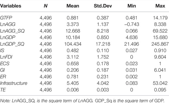
TABLE 1. Descriptive statistics of the variables.

5 Results and Discussions

5.1 The Spatiotemporal Trend of Agglomeration and Green Total-Factor Productivity

5.1.1 Time-Variation

According to the trend of AGG and GTFP during the sample period (Figure 1), it can be seen that both of these show obvious characteristics of phased changes. The sample period is divided into two stages for further analysis. The first stage (2003–2009) is a period known as the “old normal” of China’s economy. At this stage, along with the growth of economic agglomeration, the fluctuation of the GTFP declined. This is closely related to the influx of the foreign capital caused by China’s accession to the WTO in 2001 (Li M. et al., 2019). The second stage (2010–2018) is a period known as the “new normal” of China’s economy. At this stage, the AGG has a steady and declining growth trend, and the GTFP is in the stage of fluctuation, which may be related to the global financial crisis in 2008 and the transformation of China’s extensive development mode (Ying et al., 2021). Intuitively, AGG has obvious cyclical characteristics on the GTFP, which provides a preliminary basis for us to explore the nonlinear “U-shaped” impact of AGG on the GTFP.

FIGURE 1

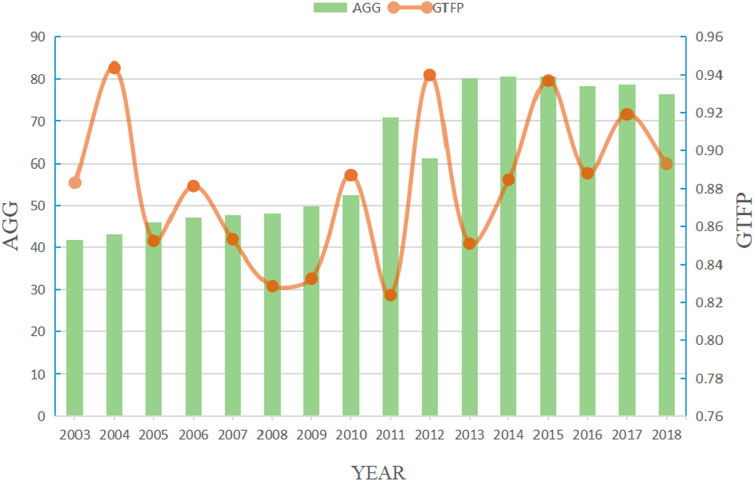
FIGURE 1. Temporal variation of the GTFP and AGG.

5.1.2 Spatial-Variation

We analyzed the spatial change characteristics of AGG and GTFP. By drawing the development trend of the AGG and GTFP during the “11th 5-Year Plan” (2006–2010) and “12th 5-Year Plan” (2011–2015) period. The reason for choosing these two time periods is that the Chinese government formulates new economic developmental strategies and policies every 5 years. In the five-year plan, the economic development strategy is relatively stable, and the observation results are more comparable.

During the “11th” period, China has set significant reduction in the total discharge of the major pollutants as a binding indicator for economic and social development. However, the overall deterioration of the environmental conditions has not yet been fundamentally curbed. It was not until the “12th” period that the effective breakthroughs were made in sustainable development. As shown in Figure 2, during the “11th” period, AGG was relatively concentrated in the core major cities. However, during the “12th” period, the AGG activities gradually spread from the eastern coastal areas to the internal areas. Shift from being concentrated in the core large cities to being concentrated in the regional central city clusters, especially in the Yangtze River Delta, Pearl River Delta, and Chengdu-Chongqing double-city economic circles. Similarly, the high-level GTFPs are mainly concentrated in the eastern coastal areas during the “11th” period. During the “12th” period, it rapidly shifted to the central and western inland areas. This trend of change is a manifestation of the transformation of China’s green economy development. AGG has promoted the transformation of economic development and has an impact on the GTFP. However, from the perspective of the matching degree between the geographical distribution of labor and the layout of the GTFP, the change of the former is relatively lagging.

FIGURE 2

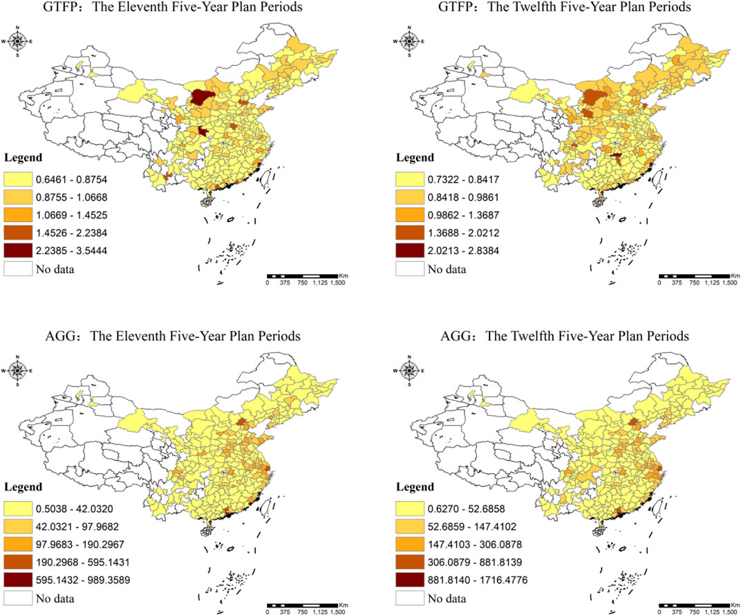
FIGURE 2. Spatial variation of the GTFP and AGG.

5.2 The Results of Spatial Econometric Estimation

The abovementioned analysis shows that there is a possible spatial correlation between the AGG and GTFP. In addition, the test results of the global Moran index prove that such spatial correlation should be taken into account in the setting of the econometric model. The value of the global Moran’s I is between −1 and 1. Positive values indicate that the variables are positively correlated in space. Table 2 shows that there is a spatial correlation between the GTFP and AGG. So, it is the right choice to use the spatial econometric model that considers spatial correlation between the variables. Therefore, we adopt a spatial econometric model to estimate the parameters.

TABLE 2

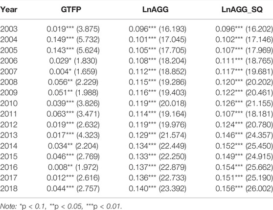
TABLE 2. Spatial autocorrelation test.

However, it is necessary to investigate whether the dynamic SDM model is suitable. According to the test results (Table 3), the spatial autocorrelation test of the OLS regression residuals shows that it is reasonable to construct a spatial measurement model. The LR test shows that the estimation results of the dynamic SDM model are robust. The Hausman test indicates that we should use the fixed-effect model.

TABLE 3

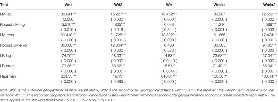
TABLE 3. Model selection checklist.

The dynamic SDM model with the spatiotemporal fixed effects was finally used, and the parameter estimation was conducted according to the error correction MLE method provided by Lee & Yu (2010). In addition, to test the necessity of introducing a dynamic model, Table 4 also lists the regression results of the static spatial Dubin model under the dual fixed effect⁵. But, we mainly analyze the results of the spatiotemporal fixed effect of the dynamic SDM.

TABLE 4

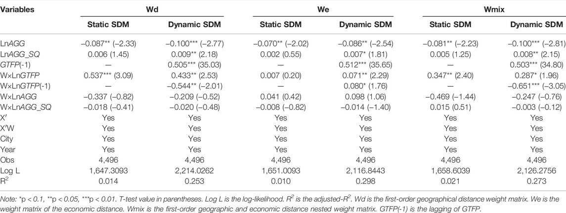
TABLE 4. Spatial econometric estimation results under different spatial matrices.

The estimated results are shown in Table 4. From the time dimension, the parameter estimates of the GTFP lagging one period are all significantly positive. The reason may be that some economic policy adjustments have a time lag (Guo et al., 2021). From the perspective of spatial dimension, there is a positive spatial correlation effect. Driven by the natural flow of the atmosphere and trade between neighboring regions, the development of the GTFP in this region is closely related to the surrounding regions. From the perspective of both time and space, the parameter estimation of the spatial lag term of the last period of GTFP is significantly negative. The possible reason is that the development of a green economy in this region has a “warning effect” on the neighboring regions.

Compared with the static SDM, the dynamic SDM has stronger explanatory power to the econometric models. In addition, according to the logarithmic likelihood value and goodness of fit in Table 4, the estimated values in the case of geographic and economic distance nested matrix are better than those in the nested matrix. Therefore, we will focus on the estimation results of the nested matrix of the dynamic SDM. It should be noted that the spatial spillover effect measured by the dynamic SDM is a global effect rather than a local effect. In this case, the point estimation results of the dynamic SDM model itself are only valid on the direction of action and significance level but do not represent the marginal impact of the explanatory variables. To investigate the influence of the explanatory variables on the explained variables, the direct and indirect effects of the explanatory variables should be further calculated based on the point estimation results (Elhorst, 2014)⁶. The direct and indirect effects can be divided into short-term effects and long-term effects from the perspective of a time dimension, respectively, reflecting the short-term impact and the long-term impact. Table 5 reports the estimation results.

TABLE 5

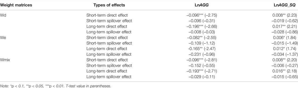
TABLE 5. The estimation result of the effect decomposition.

From the effect decomposition results in Table 5, the absolute value of the influence coefficient of most long-term effects is greater than that of the short-term effects. It shows that AGG has a more obvious long-term impact on the GTFP. In addition, there is an obvious “U-shaped” curve relationship between AGG and GTFP, which is verified by Hypothesis 1. The possible reason is that when the degree of AGG is low, there is a mismatch between the needs of the infrastructure construction and the increasing influx of labor. Economic activities are mainly manifested in the redundant construction, blind investment, and energy waste (Wang and Wang, 2019). This will cause a pressure on the local economy and the carrying capacity of the natural resources. This is similar to the research conclusion of Bashir et al. (2021). At this stage, AGG is not conducive to the promotion of GTFP.

However, as AGG continues to increase, the positive externalities brought about by agglomeration gradually appears, such as the reduction of transportation costs (Pierre et al., 2012), more employment opportunities, and increased productivity (Ines, 2020). Specifically, agglomeration can promote spatial distribution and combination optimization of labor, capital, energy, and environmental factors, and labor and capital factors have a certain substitution effect on the environmental factors, which will reduce the energy consumption and the burden on the environment (Sharma et al., 2021). Compared with a low degree of agglomeration, cities with a high degree of agglomeration can share the pollution control infrastructure. It contributes to saving pollution control costs and reducing pollution emissions. The indirect effect of AGG on GTFP is negative in the short and long term, but not significant. An insufficient level of the regional linkage may be the reason that hinders AGG from exerting spatial spillover effects.

5.3 Influence Mechanism Inspection

According to the theoretical analysis, AGG may influence the GTFP through sharing effect, structure effect, and knowledge spillover effect. To test it, we consider the following four specific factors: 1) Infrastructure sharing is measured by the urban per capita road area. 2) The green output structure is measured by the ratio of the output value of the tertiary industry to that of the secondary industry. 3) Knowledge spillover is measured by the ratio of the number of teachers in urban colleges and universities to the total labor force. 4) The level of the labor market is measured by the ratio of the number of students in urban colleges and universities to the total labor force. Furthermore, based on the classical mediating effect-test model (Chen and Lee, 2020), the following model was established for parameter estimation:

$\begin{array}{c}{Z}_{it}=\alpha +\phi Z_{it-1}+\lambda W{Z}_{it}+\theta W{Z}_{it-1}+{\rho }_{1}LnAG{G}_{it}+{\rho }_{2}WLnAG{G}_{it}\\ +X_{it}^{\prime }{\rho }_3+W{X}_{it}^{\prime }{\rho }_4+v_i+u_t+{\epsilon }_{it},\end{array}(14)$

where Z_it is the possible path. Other parameter settings are consistent with the model Eq. 10, and the control variables added in the regression are the same as that in Eq. 10. In the specific verification process, the existing control variables can be changed into mediating variables⁷.

The regression results are shown in Table 6. The direct effect estimation results show that the AGG has a U-shaped impact on infrastructure sharing, labor market advancement, and knowledge spillover. But the impact of AGG on the output structure is in an inverted “U” shape. This means that the “U-shaped” impact of AGG on the GTFP is realized through agglomeration externalities such as infrastructure sharing, labor market upgrading, and knowledge spillover. At the initial stage of agglomeration, the output structure plays a positive role, while the effect of the other three agglomeration externalities is not obvious and there are some negative effects. However, when the degree of AGG exceeds the threshold value, the positive externalities of the agglomeration begin to appear, and the improvement of the degree of agglomeration is conducive to the improvement of the GTFP.

TABLE 6

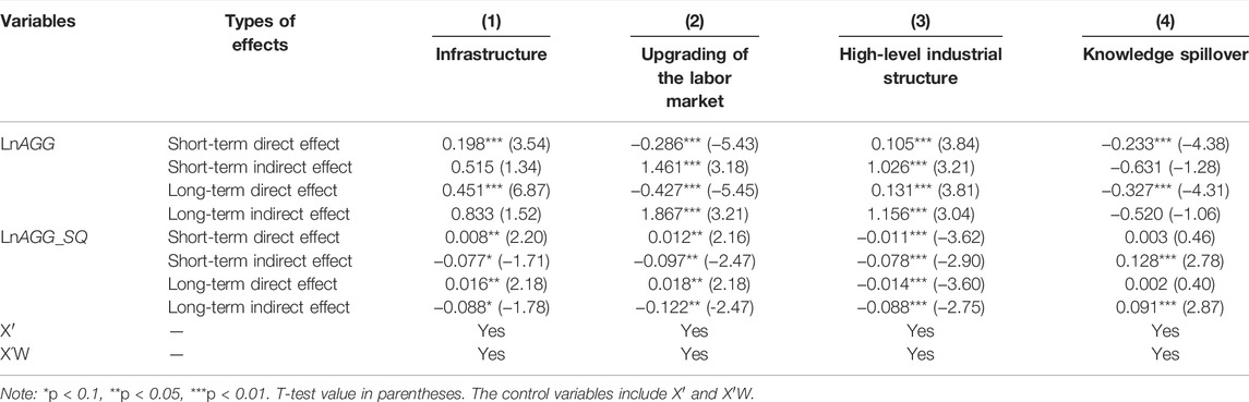
TABLE 6. The results of the mediating effect test.

5.4 Robustness Test

5.4.1 Replace the Core Explanatory Variables

The selection of the indicators is crucial to the research conclusion. It is a common practice to take employment density as the indicator to measure the degree of AGG. However, when the research sample is Chinese cities, this indicator may have some defects: According to China’s urban land-use standards, residents in the big cities are allowed to enjoy more per capita land-use area than those in small cities, which may have some influence on the measurement of AGG degree. Drawing on the practice of existing research (Shao et al., 2019), the ratio of the sum of the added value of the secondary and tertiary industries to the area is used as a new explanatory variable.

5.4.2 Replace the Spatial Weight Matrix and Remove Some Samples

In the spatial econometric model, the different weight matrices have a great influence on the estimation results. According to the geographical distance weight matrix set above, the second-order geographical distance weight matrix is further constructed, and the nested matrix of the second-order geographical distance and economic distance is considered. In addition, to avoid some unobserved and time-varying influences caused by the special administrative status of “municipalities directly under the central government”, four municipalities (Beijing, Chongqing, Shanghai, and Tianjin) are excluded.

5.4.3 Alleviate Endogeneity Problems

According to the loose assumptions of the GMM model of the dynamic panel systems, the lagged terms of the explained variables and endogenous variables can be used as instrumental variables to solve the partial endogeneity problems. Specifically, the lagged variables of the AGG and its spatial lagged items, as well as the lagged variables of GTFP and GTFP spatial lagged items, were used as instrumental variables. In addition, considering that the abovementioned methods cannot solve the inverse causal relationship between AGG and GTFP, we further use the above-constructed variables of Iv1 and Iv2.

The estimated results (Supplementary Appendix SC) show that the main results do not substantially change after changing the variable index, changing the spatial weight matrix, removing part of the samples, and alleviating the endogeneity problem.

5.5 Further Discussion

5.5.1 Industry Heterogeneity Test

Next, we distinguish between the secondary industry and the tertiary industry agglomeration. The number of workers in the secondary industry per unit of the land area is used to measure secondary industry agglomeration (AGG2). The number of people working in the tertiary industry per unit land area is used to measure tertiary industry agglomeration (AGG3). The estimated results are shown in Table 7.

TABLE 7

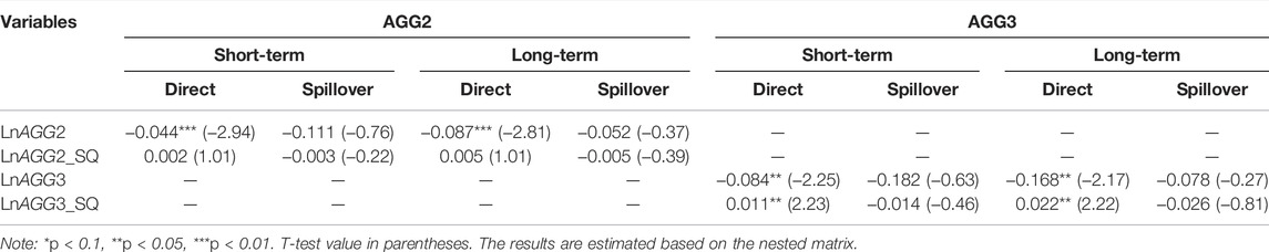
TABLE 7. The estimated results of the agglomeration by industry.

The relationship between the AGG2 and GTFP also presents a U-shaped curve. In the initial stage of agglomeration, although the rapid concentration of the economic activities has brought about the growth of economic output, the agglomeration that focuses on heavy industries has also increased energy consumption and pollutant emissions (Lan et al., 2021). In addition, when the economic production activities are mainly homogenized and low-level repeated construction, it will be difficult to produce the obvious economies of scale, knowledge spillover, and synergy effects (Wang & Wang, 2019). This is consistent with the research conclusions of Shahzad et al. (2021) and Xia et al. (2022). However, when the AGG2 has developed to a certain level, its capital-intensive characteristics will bring opportunities for development. The concentration of manpower and material resources is conducive to reducing the emission reduction costs (Yuan et al., 2020). At this stage, the agglomeration effect is enough to make up for the negative impact caused by the energy use and pollution, so it has a promoting effect on the GTFP. As far as the tertiary industry is concerned, it is mostly “green” industries such as the service industry and tourism, which use relatively little energy in the production process and emit relatively few pollutants. Similarly, there is a “U-shaped” curve relationship between the AGG3 and GTFP. However, no matter the AGG2 or the AGG3, its influence effect is limited to the local area. This is similar to the conclusion of Shahzad et al. (2022). The possible reason is that the agglomeration of the secondary and tertiary industries is of low quality, which leads to spatial mismatch between the industrial structure of the region and the surrounding areas, the disconnection between the developmental demands of the regions.

5.5.2 Regional Heterogeneity Test

China’s various regions have obvious characteristics of heterogeneity in the economic structure⁸. The division of east, middle, and west reflects the differences in the level of economic development and labor distribution among the regions. Therefore, we further divide the regional samples for parameter estimation. The results obtained are shown in Table 8.

TABLE 8

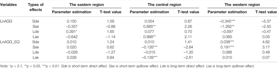
TABLE 8. Estimated results of the agglomeration by region.

According to Table 8, the relationship between AGG and GTFP still shows a “U-shaped” curve. Specifically, AGG in the eastern region does not have a significant spillover effect on the surrounding areas. As the region with the highest level of economic development in China, the eastern region has relatively abundant resources. This causes competition between the cities in the eastern region greater than cooperation (Zelai, 2009). It blocks the spatial spillover effect of the agglomeration externalities to a certain extent. The estimation result of AGG in the central region is similar to that in the eastern region. But the difference is that the AGG in the central region not only has an impact on the GTFP of the region but also has a significant spatial spillover effect on the surrounding areas. The possible reason is that the central region, as the undertaking ground of industrial transfer, needs to utilize the labor resource endowments of different cities. The close connection between the cities accelerates the spillover effect of knowledge and facility sharing. Although the economic agglomeration activities in the western region have also produced obvious spatial spillover effects, their direction of action is opposite to that in the central region. The possible reason is that the western region is more agglomerated of the secondary industries. A large and comprehensive layout can easily lead to blind investment and redundant construction (Lan et al., 2021).

5.5.3 Time-Segment Heterogeneity Test

The emergence and development of an urban system are the results of the joint action of the centripetal force and centrifugal force. For a long time, people seem to have the idea that high-density economic activities are the root cause of increased energy consumption, environmental quality, and various urban diseases. However, we hold a different view. Considering the various positive externalities of agglomeration, AGG may be an important way to realize green development. The motivation of energy conservation, emission reduction, and environmental governance may also become the “centripetal force” of AGG.

Since 2000, various provinces and cities have successively initiated the reform of the Hukou registration system. The reform aims to attract surplus rural labor to urban. The last area to implement the reforms was Chongqing (2010). To test the impact of the reform on AGG and GTFP we use 2010 as the boundary and divide the sample into two periods: 2003–2010 and 2011–2018. The impact of AGG on the dynamic space of GTFP before and after the implementation of the policy is discussed. Table 9 reports the corresponding estimation results. From the overall trend, in the two periods, the relationship between AGG and GTFP still shows a “U”-shaped curve. However, after 2010, the impact of AGG on GTFP of the surrounding areas has turned from negative to positive. From the perspective of the degree of influence, the estimated value of the effect parameter of AGG in 2003–2010 is significantly lower than that in 2011–2018. It means that since the reform of the Hukou registration system, the local governments have relaxed their obstacles to AGG. This promoted the redistribution of the economic geography, increased the degree of agglomeration, and enabled some cities to cross the threshold. This is consistent with the research conclusion of Cui et al. (2022). From the perspective of the final effect, the impact and significance of AGG on the GTFP have been further improved after the “population mobility restriction” was relaxed.

TABLE 9

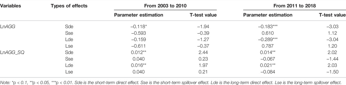
TABLE 9. Estimated results of the agglomeration by time-segment.

6 Conclusion and Policy Implications

6.1 Research Conclusion

China’s economy has made great strides, but with the economic development has come the natural resource depletion serious environmental pollution. China now ranks second globally in GDP, but it ranks first in terms of both pollutant emissions (CO₂, SO₂, PM_2.5, and oxynitride) and primary energy consumption. This has forced China to change modes from traditional development to green development. The three key factors in green development are economic development, resource conservation, and environmental protection. When rapid development occurs, the degree of economic agglomeration also increases. However, there are no consensus empirical studies about how economic agglomeration affects economic growth and environmental quality. This raises the question of how economic agglomeration will affect green economy efficiency, as measured by an index that comprehensively considers economic growth, resource conservation, and environmental protection. The answer to this question will help formulate industrial policies, achieve the goals of energy conservation and emission reduction, and contribute to China’s sustainable future development.

We have constructed a theoretical model that can describe the relationship between economic agglomeration and green TFP. Under the super-efficiency DEA framework, the NDDF is used to calculate a green TFP that comprehensively considers economic growth, resource conservation, and environmental protection. The panel data of 281 prefecture-level and abovementioned cities in China from 2003 to 2018 are used. Based on the quantitative analysis techniques such as the dynamic SDM model and mediation effect model, the impact of the economic agglomeration on the green TFP and the spatial spillover effect is tested. Several possible influence paths have been found and verified. Finally, robustness test and heterogeneity analysis were carried out. The results are as follows:

1) The green TFP has a strong space-time dependence effect. In the time dimension, if the green TFP of the previous period was at a high level, the next period may also continue to rise. In the spatial dimension, the green TFP between the regions shows a significant positive spatial correlation effect. In terms of time and space, the current poor performance of the green TFP in this region has a clear “warning effect” on the next green TFP development in the neighboring regions.

2) The impact of economic agglomeration on the green TFP has two ways, direct and indirect. As far as the direct impact is concerned, the relationship between economic agglomeration and green TFP both shows an obvious “U”-shaped curve. When the degree of economic agglomeration is low, the gathering suppresses the green TFP. But when the economic agglomeration exceeds the threshold, it shows a clear promotion effect on the green TFP. As far as indirect effects are concerned, “low-quality agglomeration of the secondary and tertiary industries” and “restrictions on the population mobility” are important reasons that economic agglomeration fails to produce a positive spatial spillover effect on the surrounding areas.

3) Economic agglomeration has a threshold effect on the impact of agglomeration externalities such as infrastructure sharing, knowledge spillover, and advanced labor market. This is the inherent reason for the “U-shaped” curve relationship between economic agglomeration and green TFP. When the degree of economic agglomeration is low, the abovementioned three types of agglomeration externalities are not yet obvious. When the degree of agglomeration exceeds the threshold, these three paths can play a vital role in promoting the effective communication and exchange of information, reducing the cost of information transmission, promoting the formation of economies of scale, and controlling pollutants.

6.2 Policy Implications

The policy implications of the abovementioned conclusions are embodied in the following two aspects.

1) We should promote the rational allocation of the human resources in space. The traditional concept believes that the agglomeration of economic activities is the root cause of the increase in energy consumption and environmental pollution. This view weakens the potential energy-saving and emission reduction effects of economic agglomeration itself. Our conclusions show that when the economic agglomeration reaches a certain level, the spatially concentrated production mode of the economic activities has obvious green attributes compared to the dispersed production mode. This means that the city’s economic development strategy and green transformation goals can achieve wonderful implementation effects under certain conditions. At present, problems such as high energy consumption and high pollution in cities are more prominent. This may be because the economic agglomeration is at a low-level stage, and its positive externalities are not yet obvious. We believe that as the level of economic agglomeration continues to increase, its inherent green effect will appear on a larger scale. Therefore, we should continue to promote the development of an agglomeration economy and promote the formation of a coordinated linkage mechanism between the regions. The spatial concentration of the economic activities is increased, and economic agglomeration is brought to an ideal stage where it can exert a significant green effect.

2) A green development strategy is formulated rationally based on the characteristics of the city. In the small city, it is necessary to rely on the surrounding large and medium cities to develop a green economy through the improvement of urban infrastructure construction and industrial cooperation. For the medium-sized cities, resource and infrastructure carrying capacity must be considered. Attention should be paid to cultivating the momentum of urban agglomerations. It should take resource conservation and environmental friendliness as the prerequisite and promote moderate-scale urbanization through the reform of the Hukou registration system. For the large cities, it is necessary to promote integrated development of cities and towns, exerting the gathering effect and divergence function. The agglomeration effect brought about by the concentration of economic activities by improving the allocation of the urban public resources is maximized.

However, regardless of the positive results, there are still some limitations. Green TFP is a complex system with multiple levels and multiple structures. The index calculated by the NDDF model is a simple simulation of the entire system, and further research is needed to develop a more robust evaluation system. In addition, as the application of the green TFP indicators, its impact on sustainable development is also an area of related research. Many areas can be further studied in the future, such as the impact on poverty alleviation and ecological optimization.

Data Availability Statement

The original contributions presented in the study are included in the article/Supplementary Material, further inquiries can be directed to the corresponding author.

Author Contributions

Conception and design of the study: HA-m and TJ-y. Acquisition of data: RZ and TJ-y. Analysis and interpretation of data: TJ-y. Drafting the manuscript: TJ-y. Revising the manuscript critically for important intellectual content: HA-m and TJ-y.

Funding

This research was supported by the National Social Science Foundation of China (Project No. 19BJY130).

Conflict of Interest

The authors declare that the research was conducted in the absence of any commercial or financial relationships that could be construed as a potential conflict of interest.

Publisher’s Note

All claims expressed in this article are solely those of the authors and do not necessarily represent those of their affiliated organizations, or those of the publisher, the editors, and the reviewers. Any product that may be evaluated in this article, or claim that may be made by its manufacturer, is not guaranteed or endorsed by the publisher.

Supplementary Material

The Supplementary Material for this article can be found online at: https://www.frontiersin.org/articles/10.3389/fenvs.2022.829160/full#supplementary-material

Footnotes

¹The LR test result is shown in Table 3.

²The complete process is shown in Supplementary Appendix S1.

³The formula is: $K_{it}^s=K_{it}^f+\left(1-\delta \right)K_{i,t-1}^s,K_{i\text{0}}^s=K_{i\text{0}}^f/\left(g+\delta \right)$, where K_its and K_itf represent the capital stock and fixed asset investment of the city i in the t year. Subplot 0 is the initial year. δ is the depreciation rate, taking 8.5%. g is the average annual growth rate of the fixed asset investment of the selected sample cities.

⁴The website of the Geographic Information Resources Directory Service System is: https://www.webmap.cn/main.do?method=index.

⁵Compared with the static SDM model which only contains the GTFP, the dynamic SDM model also has both the time lag effect and space-time double lag effect.

⁶The direct effect refers to the impact of economic agglomeration on the green TFP in the region, which includes the feedback effect. However, due to its small value, generally, it can be ignored; indirect effect refers to the influence of the change of a local factor on the green TFP in the neighboring area, namely, the spatial spillover effect of an influencing factor.

⁷For example, when the transmission path is “infrastructure”, the variable from the control variable is removed and used as an intermediate variable.

⁸Three areas are, respectively, the most populated in the developed economic times of the central region, relatively densely populated but the most economically developed of eastern areas and the less developed western region relatively sparse population and economy.

References

Balaguer, J., and Cantavella, M. (2018). The Role of Education in the Environmental Kuznets Curve. Evidence from Australian Data. Energ. Econ. 70, 289–296. doi:10.1016/j.eneco.2018.01.021

CrossRef Full Text | Google Scholar

Banerjee, A., Duflo, E., and Qian, N. (2020). On the Road: Access to Transportation Infrastructure and Economic Growth in China. J. Dev. Econ. 145, 102442. doi:10.1016/j.jdeveco.2020.102442

CrossRef Full Text | Google Scholar

Bashir, M. F., Ma, B., Shahbaz, M., Shahzad, U., and Vo, X. V. (2021). Unveiling the Heterogeneous Impacts of Environmental Taxes on Energy Consumption and Energy Intensity: Empirical Evidence from OECD Countries. Energy 226, 120366. doi:10.1016/j.energy.2021.120366

CrossRef Full Text | Google Scholar

Brülhart, M., and Mathys, N. A. (2008). Sectoral Agglomeration Economies in a Panel of European Regions. Reg. Sci. Urban Econ. 38 (4), 348–362. doi:10.1016/j.regsciurbeco.2008.03.003

CrossRef Full Text | Google Scholar

Cai, X., Lu, Y., Wu, M., and Yu, L. (2016). Does Environmental Regulation Drive Away Inbound Foreign Direct Investment? Evidence from a Quasi-Natural Experiment in China. J. Dev. Econ. 123, 73–85. doi:10.3386/w1789710.1016/j.jdeveco.2016.08.003

CrossRef Full Text | Google Scholar

Chen, Y., and Lee, C.-C. (2020). Does Technological Innovation Reduce CO2 emissions?Cross-Country Evidence. J. Clean. Prod. 263, 121550. doi:10.1016/j.jclepro.2020.121550

CrossRef Full Text | Google Scholar

Chen, Z. M. (1993). On the Principle, Contents and Methods Used to Compile the Chinese Geomorphological Maps——Taking The 1: 4,000,000 Chinese Geomorphological Map as An Example. Acta Geographica Sinica (02), 105–113.

Google Scholar

Chen, W. Y., Hu, F. Z. Y., Li, X., and Hua, J. (2017). Strategic Interaction in Municipal Governments' Provision of Public Green Spaces: A Dynamic Spatial Panel Data Analysis in Transitional China. Cities 71, 1–10. doi:10.1016/j.cities.2017.07.0033

CrossRef Full Text | Google Scholar

Cheng, Z., Li, L., and Liu, J. (2018). Industrial Structure, Technical Progress and Carbon Intensity in China's Provinces. Renew. Sust. Energ. Rev. 81, 2935–2946. doi:10.1016/j.rser.2017.06.103

CrossRef Full Text | Google Scholar

Cheng, Z. (2016). The Spatial Correlation and Interaction between Manufacturing Agglomeration and Environmental Pollution. Ecol. Ind. 61 (2), 1024–1032. doi:10.1016/j.ecolind.2015.10.060

CrossRef Full Text | Google Scholar

Ciccone, A., and Hall, R. (1996). Productivity and the Density of Economic Activity. Am. Econ. Rev. 86 (1), 54–70. doi:10.3386/w4313

CrossRef Full Text | Google Scholar

Cui, L., Weng, S., Nadeem, A. M., Rafique, M. Z., and Shahzad, U. (2022). Exploring the Role of Renewable Energy, Urbanization and Structural Change for Environmental Sustainability: Comparative Analysis for Practical Implications. Renew. Energ. 184, 215–224. doi:10.1016/j.renene.2021.11.075

CrossRef Full Text | Google Scholar

Daniel, J. G. (2007). Agglomeration, Productivity, and Transport Investment. J. Transport Econ. Pol. 41 (3), 317–343. stable/20054024. doi:10.1787/234743465814

CrossRef Full Text | Google Scholar

Drucker, J., and Feser, E. (2012). Regional Industrial Structure and Agglomeration Economies: An Analysis of Productivity in Three Manufacturing Industries. Region. Sci. Urban Econ. 42 (1-2), 1–14. doi:10.1016/j.regsciurbeco.2011.04.006

CrossRef Full Text | Google Scholar

Elhorst, J. P. (2010). Applied Spatial Econometrics: Raising the Bar. Spat. Econ. Anal. 5 (1), 9–28. doi:10.1080/17421770903541772

CrossRef Full Text | Google Scholar

Elhorst, J. P. (2014). Matlab Software for Spatial Panels. Int. Reg. Sci. Rev. 37 (3), 389–405. doi:10.1177/0160017612452429

CrossRef Full Text | Google Scholar

Ertur, C., and Koch, W. (2007). Growth, Technological Interdependence and Spatial Externalities: Theory and Evidence. J. Appl. Econom. 22 (6), 1033–1062. doi:10.1002/jae

CrossRef Full Text | Google Scholar

Feng, Z. M., Tang, Y., Yang, Y. Z., and Zhang, D. (2007). The Relief Degree of Land Surface in China and Its Correlation with Population Distribution. Acta Geographica Sinica (10), 1073–1082.

Google Scholar

Greenstone, M., Hornbeck, R., and Moretti, E. (2010). Identifying Agglomeration Spillovers: Evidence From Winners and Losers of Large Plant Openings. J. Polit. Economy 118 (3), 536–598. doi:10.1086/653714

CrossRef Full Text | Google Scholar

Guo, J., Zhou, Y., Ali, S., Shahzad, U., and Cui, L. (2021). Exploring the Role of Green Innovation and Investment in Energy for Environmental Quality: An Empirical Appraisal From Provincial Data of China. J. Environ. Manage. 292, 112779. doi:10.1016/j.jenvman.2021.112779

PubMed Abstract | CrossRef Full Text | Google Scholar

Helm, I. (2020). National Industry Trade Shocks, Local Labour Markets, and Agglomeration Spillovers. Rev. Econ. Stud. 87 (3), 1399–1431. doi:10.1093/restud/rdz056

CrossRef Full Text | Google Scholar

Krugman, P. (1998). Space: The Final Frontier. J. Econ. Perspect. 12 (2), 161–174. doi:10.1257/jep.12.2.161

CrossRef Full Text | Google Scholar

Lan, F., Sun, L., and Pu, W. (2021). Research On the Influence of Manufacturing Agglomeration Modes On Regional Carbon Emission and Spatial Effect in China. Econ. Model. 96, 346–352. doi:10.1016/j.econmod.2020.03.016

CrossRef Full Text | Google Scholar

Lee, L.-f., and Yu, J. (2010). A Spatial Dynamic Panel Data Model with Both Time and Individual Fixed Effects. Econom. Theor. 26 (2), 564–597. doi:10.1017/S0266466609100099

CrossRef Full Text | Google Scholar

Li, J. L., and Xu, B. (2018). Curse or Blessing: How Does Natural Resource Abundance Affect Green Economic Growth China? Econ. Res. J. 53 (09), 151–167.

Google Scholar

Li, M., Patiño-Echeverri, D., and Zhang, J. (2019). Policies to Promote Energy Efficiency and Air Emissions Reductions in China's Electric Power Generation Sector During the 11Th and 12Th Five-Year Plan Periods: Achievements, Remaining Challenges, and Opportunities. Energy Policy 125, 429–444. doi:10.1016/j.enpol.2018.10.008

CrossRef Full Text | Google Scholar

Li, Z., Dong, H., Huang, Z., and Failler, P. (2019). Impact of Foreign Direct Investment On Environmental Performance. Sustainability 11 (13), 3538. doi:10.3390/su11133538

CrossRef Full Text | Google Scholar

Lin, B., and Chen, Z. (2018). Does Factor Market Distortion Inhibit the Green Total Factor Productivity in China? J. Clean. Prod. 197 (1), 25–33. doi:10.1016/j.jclepro.2018.06.094

CrossRef Full Text | Google Scholar

Lin, B., and Du, K. (2015). Energy and CO2 emissions performance in China's regional economies: Do market-oriented reforms matter? Energy Policy 78 (3), 113–124. doi:10.1016/j.enpol.2014.12.025

CrossRef Full Text | Google Scholar

Lin, B. Q., and Liu, H. X. (2015). Do Energy and Environment Efficiency Benefit from Foreign Trade ?——The Case of China's Industrial Sectors. Econ. Res. J. 50 (09), 127–141.

Google Scholar

Liu, S., Zhu, Y., and Du, K. (2017). The Impact of Industrial Agglomeration On Industrial Pollutant Emission: Evidence From China Under New Normal. Clean. Techn Environ. Pol. 19 (9), 2327–2334. doi:10.1007/s10098-017-1407-0

CrossRef Full Text | Google Scholar

Pierre, P. C., Gilles, D., Laurent, G., Diego, P., and Sébastien, R. (2012). The Productivity Advantages of Large Cities: Distinguishing Agglomeration From Firm Selection. Econometrica 80 (6), 2543–2594. doi:10.3982/ECTA8442

CrossRef Full Text | Google Scholar

Ren, S., Li, X., Yuan, B., Li, D., and Chen, X. (2018). The Effects of Three Types of Environmental Regulation On Eco-Efficiency: A Cross-Region Analysis in China. J. Clean. Prod. 173, 245–255. doi:10.1016/j.jclepro.2016.08.113

CrossRef Full Text | Google Scholar

Ren, W., Zhong, Y., Meligrana, J., Anderson, B., Watt, W. E., Chen, J., et al. (2003). Urbanization, land use, and water quality in Shanghai. Environ. Int. 29 (5), 649–659. doi:10.1016/S0160-4120(03)00051-5

PubMed Abstract | CrossRef Full Text | Google Scholar

Shahzad, U., Ferraz, D., Nguyen, H.-H., and Cui, L. (2022). Investigating the Spill Overs and Connectedness Between Financial Globalization, High-Tech Industries and Environmental Footprints: Fresh Evidence in Context of China. Technol. Forecast. Soc. Change 174, 121205. doi:10.1016/j.techfore.2021.121205

CrossRef Full Text | Google Scholar

Shahzad, U., Schneider, N., and Ben Jebli, M. (2021). How Coal and Geothermal Energies Interact with Industrial Development and Carbon Emissions? An Autoregressive Distributed Lags Approach to the Philippines. Resour. Pol. 74, 102342. doi:10.1016/j.resourpol.2021.102342

CrossRef Full Text | Google Scholar

Shao, S., Zhang, K., and Dou, J. M. (2019). Effects of Economic Agglomeration on Energy Saving and Emission Reduction: Theory and Empirical Evidence from China. Manag. World 35 (01), 36–60+226.

Google Scholar

Sharma, G. D., Shah, M. I., Shahzad, U., Jain, M., and Chopra, R. (2021). Exploring the Nexus Between Agriculture and Greenhouse Gas Emissions in BIMSTEC Region: The Role of Renewable Energy and Human Capital as Moderators. J. Environ. Manage. 297, 113316. doi:10.1016/j.jenvman.2021.113316

PubMed Abstract | CrossRef Full Text | Google Scholar

Song, M., Xie, Q., and Shen, Z. (2021). Impact of Green Credit On High-Efficiency Utilization of Energy in China Considering Environmental Constraints. Energy Policy 153, 112267. doi:10.1016/j.enpol.2021.112267

CrossRef Full Text | Google Scholar

Stern, D. I. (2004). The Rise and Fall of the Environmental Kuznets Curve. World Dev. 32 (8), 1419–1439. doi:10.1016/j.worlddev.2004.03.004

CrossRef Full Text | Google Scholar

Sun, P., and Yuan, Y. (2015). Industrial Agglomeration and Environmental Degradation: Empirical Evidence in Chinese Cities. Pac. Econ. Rev. 20 (4), 544–568. doi:10.1111/1468-0106.12101

CrossRef Full Text | Google Scholar

Wang, N., Zhu, Y., and Yang, T. (2020). The Impact of Transportation Infrastructure and Industrial Agglomeration On Energy Efficiency: Evidence From China'S Industrial Sectors. J. Clean. Prod. 244, 118708. doi:10.1016/j.jclepro.2019.118708

CrossRef Full Text | Google Scholar

Wang, X., Sun, C., Wang, S., Zhang, Z., and Zou, W. (2018). Going Green or Going Away? A Spatial Empirical Examination of the Relationship between Environmental Regulations, Biased Technological Progress, and Green Total Factor Productivity. Ijerph 15 (9), 1917. doi:10.3390/ijerph15091917

PubMed Abstract | CrossRef Full Text | Google Scholar

Wang, Y., and Wang, J. (2019). Does Industrial Agglomeration Facilitate Environmental Performance: New Evidence From Urban China? J. Environ. Manage. 248, 109244. doi:10.1016/j.jenvman.2019.07.015

PubMed Abstract | CrossRef Full Text | Google Scholar

Xia, W., Apergis, N., Bashir, M. F., Ghosh, S., Doğan, B., and Shahzad, U. (2022). Investigating the Role of Globalization, and Energy Consumption for Environmental Externalities: Empirical Evidence From Developed and Developing Economies. Renew. Energ. 183, 219–228. doi:10.1016/j.renene.2021.10.084

CrossRef Full Text | Google Scholar

Ying, L., Li, M., and Yang, J. (2021). Agglomeration and Driving Factors of Regional Innovation Space Based On Intelligent Manufacturing and Green Economy. Environ. Tech. Innovation 22, 101398. doi:10.1016/j.eti.2021.101398

CrossRef Full Text | Google Scholar

Yuan, H., Feng, Y., Lee, C.-C., and Cen, Y. (2020). How Does Manufacturing Agglomeration Affect Green Economic Efficiency? Energ. Econ. 92, 104944. doi:10.1016/j.eneco.2020.104944

CrossRef Full Text | Google Scholar