Application of Soft Computing in Predicting Groundwater Quality Parameters

Evaluating the quality of groundwater in a specific aquifer could be a costly and time-consuming procedure. An attempt was made in this research to predict various parameters of water quality called Fe, Cl, SO₄, pH and total hardness (as CaCO₃) by measuring properties of total dissolved solids (TDSs) and electrical conductivity (EC). This was reached by establishing relations between groundwater quality parameters, TDS and EC, using various machine learning (ML) models, such as linear regression (LR), tree regression (TR), Gaussian process regression (GPR), support vector machine (SVM), and ensembles of regression trees (ER). Data for these variables were gathered from five unrelated groundwater quality studies. The findings showed that the TR, GPR, and ER models have satisfactory performance compared to that of LR and SVM with respect to different assessment criteria. The ER model attained higher accuracy in terms of R² in TDS 0.92, Fe 0.89, Cl 0.86, CaCO₃ 0.87, SO₄ 0.87, and pH 0.86, while the GPR model attained an EC 0.98 compared to all developed models. Moreover, comparisons among the different developed models were performed using accuracy improvement (AI), improvement in RMSE (PRMSE), and improvement in PMAE to determine a higher accuracy model for predicting target properties. Generally, the comparison of several data-driven regression methods indicated that the boosted ensemble of the regression tree model offered better accuracy in predicting water quality parameters. Sensitivity analysis of each parameter illustrates that CaCO₃ is most influential in determining TDS and EC. These results could have a significant impact on the future of groundwater quality assessments.

Introduction

The rising need for clean drinking water draws awareness for the management of groundwater quality. The alteration in groundwater quality because of natural substances in addition to anthropogenic activities in the surrounding soil could indicate repercussions on public health if left without treatment (Basim et al., 2018). An awareness of factors that influence groundwater quality is vital to assessing the potability of water in a specific area. Nevertheless, the quality of a specific groundwater resource is connected to it as a natural constituent, for example, the several microorganisms, sediments, and chemical compounds that exist in it. Chemicals in groundwater could originate from various resources, including precipitation, runoff, and the material of the surrounding rock. The significance that water–rock interactions play in the chemical composition of groundwater is examined in detail by Lloyd and Heathcote, (1985). Human health is mostly affected from pathogens and chemicals in the water source (Schmoll et al., 2006)^, The World Health Organization has been publishing and updating the guidelines and standards for all chemicals or metals, which may be of concern for groundwater quality valuations (World Health Organization, 1993). Most of the parameters in water, which are not inclined to cause health issues, even in higher concentrations, are fine for consumption, whereas others could be dangerous at insignificant concentrations. Chloride (Cl), for example, may lead to changes in savor; nonetheless, it is not poisonous to humans. Moreover, it might cause corrosion of metals in the well and pipe if it occurs at concentrations higher than 250 mg/L. Iron (Fe) has the same effect, in which it affects the groundwater quality, mostly esthetically, changing its savor and appearances. In several examples, the existence of iron is more of an advantage than a disadvantage due to its importance in human nurture. Sulfate (SO₄) concentration may be highly dangerous to human health among the studied ions. Concentrations of 1,000–1,200 mg/L display a laxative impact when consumed. Therefore, the WHO recommends that health authorities be alerted at concentrations greater than 500 mg/L. The total hardness of groundwater could be eroded at concentrations less than 100 mg/L of CaCO₃ and drive an increase in sedimentation at concentrations exceeding 200, dependent on pH. However, some investigations have demonstrated a probable reverse relation between hardness and cardiovascular infection. Like domestic water supplies, chemicals in agricultural systems could bring about benign, esthetic impacts or more toxic, destructive impacts. Evaluating groundwater quality could be an engaging process. Reliant on the size of a specific resource and the site of wells, several samples may be required to establish a representative quality evaluation. After the sampling process is completed, there is frequent requirement for off-site laboratory analysis to determine the concentration of several ions. In contrast, measures of water quality, such as pH, total dissolved solids (TDSs), and electrical conductivity (EC), could be simply measured on-site using digital meters.

Techniques for evaluating groundwater quality vary depending on the quantity of interest. Chemical and physical characteristics such as EC, pH, and TDS can often be measured on-site with digital meters. Concentrations of most dissolved anions and cations need to be analyzed off-site in laboratory settings using flame atomic absorption spectrophotometric methods. Concentrations of relevant anions such as fluoride, chloride, nitrate, nitrite, and sulfate can be measured similarly to ion chromatographs. These instruments can be costly and time-intensive. Consequently, considering that adopting an alternative method for quick, on-site analysis is necessary, machine learning models allow us to develop software solutions for all these problems and are much cheaper than this off-site laboratory. Therefore, it will examine which of the machine learning methods of calculating groundwater quality produces more reliable and consistent final models. Observing this research gap, this study presents the solution of the following research questions:

a) Can machine learning models predict TDS and EC, Fe, Cl, SO₄, CaCO_3, and pH? In addition, the most efficient techniques of groundwater quality prediction are provided to help make decisions toward better water resource planning and management.

b) What results will comparison of various machine learning models yield in the prediction of TDS and EC, Fe, Cl, SO₄, CaCO₃, and pH?

c) What is the sensitivity of the developed models to different input groundwater quality parameters in the prediction of TDS and EC?

Consequently, this study proposed that the time and effort needed for off-site analysis can be reduced if a functional relation is established between these simply measured parameters and concentrations of ions in groundwater. In the current study, five machine learning techniques, linear regression (LR), tree regression (TR), Gaussian process regression (GPR), support vector machine (SVM), and ensembles of regression trees (ER), were developed to predict the concentrations of Fe, Cl, SO₄, pH, and CaCO₃ from measurements of TDS and EC as well as predict TDS and EC from measurements of Fe, Cl, SO₄, CaCO₃, and pH parameters.

Literature Review

For groundwater modeling, machine learning (ML) methods are being acceptable and robust when applying different machine learning models to predict the groundwater level (Rajaee et al., 2019). Regarding water quality forecasting, some studies have used ML methods, as reviewed by TiyashaTung et al., (2020). In the study by Lu and Ma, (2020),^, an extreme gradient boosting model and random forest (RF) model were used to forecast six water quality statistics in the Tualatin River. Castrillo and García, (2020) applied linear and RF models to estimate a highly regular nutrient concentration in river Thames. Importantly, physical parameters, such as EC, pH, and temperature, which could be measured via sensor technologies as predictors, could improve ML efficiency, as in the study by Ayadi et al., (2019); Chowdury et al., (2019). Thus, decision makers can be encouraged to apply ML techniques for planning and management of water quality. However, it is important to examine the ML methods for predicting groundwater quality parameters using only a physical parameter as the input variable without depending on decreasing model performance by applying a past dataset. The applications of ML models have been used for prediction and evaluated irrigation of the water quality index (WQI) of aquifer systems applying physical parameters as features as in the study by El Bilali et al., (2021); they developed and evaluated Artificial Neural Network (ANN), RF, Adaptive Boosting (Adaboost), and SVM methods using 520 samples of the data set related to 14 parameters of groundwater quality in Morocco. In general, the outcomes showed that the predictive performance of the adaptive boosting and random forest methods was better than that of the other models. However, adaptive boosting also has a few drawbacks. For instance, it is from experimental evidence and is especially vulnerable to uniform noise. Weak classifiers that are too weak could lead to low margins and overfitting. Shadrin et al., (2021) proposed a method to build a weight WQI and the spatial predicting map of the WQI in the testing zone. The WQI was computed using the dimensionality decrease method, and a spatial map of the WQI was built applying GPR. Thus, WQI estimation was used to build a spatial distribution model, and the GPR-BIC method was compared with universal kriging (UK), with exponential, ordinary kriging (OK), Gaussian kernel, polynomial kernel, and periodic kernel. The performance of each model was evaluated, and the findings showed that the BIC-GPR model offered superior performance compared with other models. This study (Knoll et al., 2017) composes spatial predictors with respective monitoring sites and utilizes various designs of contribution zones. Their impacts on the performance of many statistical models were examined. They compared multiple linear regression (MLR), classification and regression tree (CART), RF, and ER in terms of the prediction performance of every model with respect to several objective functions, and the outcomes indicated that the RF model outperformed the other models. In the study by Khalil et al., (2005)^, some models were used to predict contaminant levels in groundwater relevance vector machines (RVMs), ANNs, SVMs, and local weight projecting regression (LWPR), and their findings demonstrated the capability of ML to build accurate models with robust predictive abilities. Thus, this motivates us to further investigate the application of GPR, SVMs, RF, and MLR models in this study. Vijay and Kamaraj, (2019) address the physicochemical characteristics of groundwater quality in Vellore district. The bore wells from which samples were gathered are widely utilized for drinking purposes. Water quality variables, such as pH, TDS, EC, Cl, SO₄, nitrate, carbonate, bicarbonate, metal ions, and trace elements, have been predicted (Ighalo et al., 2021). They emphasized predicting water quality by using the ML classifier algorithm C5.0, naïve Bayes, and RF as leaners for water quality prediction with high precision and effectiveness. Singha et al., (2021) used a deep learning (DL)–based model to predict ground water quality and compared it with various machine learning approaches, such as RF, ANN, and eXtreme gradient boosting (XGBoost). A total of 226 ground water sets were collected from an agriculturally intensive zone in India, and their findings indicated that the DL method provided a better prediction with high accuracy in predicting groundwater quality. However, the DL technique has the disadvantage of requiring a very large amount of data to perform more accurately than other approaches. Although ensemble models in hydrological prediction often outperform ordinary ML techniques, their performance in ground water quality modeling has not been investigated. In this study, our effort is to contribute to overcoming the limitations of traditional methods by using ML models to predict groundwater quality.

Materials and Method

Description of the Data

The datasets used in the current study are available online (Calvert, 2020) and were gathered from five unrelated groundwater quality studies. A collective set of 206 samples of the groundwater quality dataset was collected (datasets I–V). Numerous samples were excluded from the evaluation because of the existence of a statistical outlier in one or various parameters. The iron dataset, highly remarkably, included a sum of 39 samples that were lower than the finding limit and were verified = 0. These samples were ignored in cases where iron was utilized for evaluation, bringing the size of the applied dataset in those cases to 158 samples. Datasets that did not measure overall hardness (III and IV) were computed from calcium and magnesium concentrations utilizing the equation (Crittenden et al., 2012) below.

$Hardness,\frac{eq}{l}=2\left[C{a}^2\right]+2\left[M{g}^2\right]\text{.}(1)$

For the complete, unabridged dataset, Table 1 provides a simple statistic of each parameter.

TABLE 1

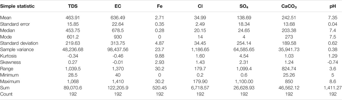
TABLE 1. Summary of simple statistics of data.

Machine Learning Models

Linear regression models (LR): This is a systematic technique for adding and removing terms from linear or generalizing linear models based on their statistical importance in describing a target variable. At every step, the technique search for terms to add or remove from the model depends on the value of the criterion argument. Generally, linear regression models can be defined as follows:

$y_i={\beta }_0+{\displaystyle \sum }_{m=1}^m{\beta }_m{f}_m\left(X_{i1},X_{i2},\cdots ,X_{ip}\right)+{\epsilon }_i,i=1,\cdots ,n,(2)$

where $y_i$ represents $ith$ target, ${\beta }_m$ is $mth$ coefficient, $"{\beta }_0$ is a constant term in model”, $X_{i\text{j}}$ refer to $ith$ observations on $jth$ predictor variable (j = 1,⋯,p), and ${\epsilon }_i$ is $ith$ noise term for arbitrary errors, whereas $f$ represents the scalar value function of independent variable $X_{i\text{j}}$, that may be in any form involving nonlinear function or polynomial (Kutner et al., 2005; García et al., 2015). Four various kinds of LR models (linear, robust linear, interaction linear, and stepwise) will be investigated to verify which model generates the greatest outcome with the dataset. A linear term will be selected for the linear and robust models and an interaction term for the interaction linear model. According to the stepwise model, the linear interactions and 1,000 for the primary term, upper bound on the term, and highest number of steps will be set, respectively.

Tree regression models (TRs): TRs are a nonparametric supervised learning algorithm with short memory use, and the standard classification and regression tree (CART) algorithm is applied by defaulting. To prevent overfitting, a smaller tree with fewer larger leaves could be tried initially, and later, a larger tree will be considered. Three various kinds of regression trees model “fine, medium, and coarse” trees within various lowest leaf sizes. Generally, the fine tree model with small leaves indicates better accuracy on a trained dataset; however, it may reveal equivalent accuracy on the independent testing sample. On the other hand, coarse trees with large leaves do not deliver high precision to the training dataset; however, training accuracy could be used for the representative testing dataset. The regression trees that we will use in the current study are binary, and every step in prediction included examining the value of one predictor parameter. The lowest leaf size will be 4, 12, and 36 for fine trees, medium trees, and coarse trees, respectively (Kim et al., 2020).

Gaussian process regression (GPR) models: these models are nonparametric kernel-based probabilistic models. Consider a training sample {($x_a$, $y_a$); $a=\mathrm{1,2},\mathrm{..},n\},$ where $x_a$ ∈ℝk and $y_a$ ∈ℝ, derived from the undetermined distribution. The GPR technique addresses the question of prediction values of the target variable $y_{new}$, provides a new input vector $x_{new}$, and trains the dataset. The linear regression model is defined as follows:

$y=xT\beta +\epsilon .(3)$

Here, $\epsilon \sim N(0,\sigma 2).$ Error variance σ2 and coefficient β represent estimates from the dataset. The GPR approach describes the target by presenting a latent variable, $f\left(x_a\right),a=\mathrm{1,2},\mathrm{..},n$, from the GP and explicating the basis function h. The covariance functions of the latent variable capture the flatness of a target, and the basis function projects input x to a p-dimensional feature space. If $\{f\left(x\right),x\in \mathrm{ℝ}k\}$ is the GP, n observations are later delivered $x1,x2,\mathrm{..},xn;$ the combined distribution of a random variable is Gaussian. The Gaussian processes are specified via the mean m(x) and covariance functions, $d(x,x\text{′})$. That is, when $\{f\left(x\right),x\in \mathrm{ℝ}k\}$ is the GP, $E\left(f\left(x\right)\right)=m\left(x\right)$ and $Cov[f\left(x\right),f\left(x\text{′}\right)]=E\left[\{f\left(x\right)-m\left(x\right)\}\{f\left(x\text{′}\right)-m\left(x\text{′}\right)\}\right]=k(x,x\text{′})$. Now considering a next model:

$h\left(x\right)T\beta +f\left(x\right).(4)$

Here, $f\left(x\right)\sim GP(0,d(x,x\text{′}))$, which is f(x) from 0 means Gaussian Process with covariance functions, $d(x,x\text{′}).h\left(x\right)$ are the sets of basis function which transform an initial feature vector x in $R^k$ into a new feature vector h(x) in $R^p$. β is the p-by-1 vector of basis function coefficients. The example of target y could be modeling by

$P(ya|f\left(x_a\right),x_a)\sim N(y_a|h\left(x_a\right)T\beta +f\left(x_a\right),{\sigma }^2).(5)$

Then, there is a latent variable $f\left(x_a\right)$ presented for all observations $x_a$ that makes GPR models nonparametric. In the vector form, that model is equal to

$P(y|f,X)\sim N(y|H\beta +f,{\sigma }^{2}I).(6)$

Here,

$X=\left(\begin{array}{c}\begin{array}{c}x{T}_1\\ x{T}_2\\ ⋮\end{array}\\ x{T}_n\end{array}\right),y=\left(\begin{array}{c}\begin{array}{c}{y}_1\\ y_2\\ ⋮\end{array}\\ y_n\end{array}\right),H=\left(\begin{array}{c}\begin{array}{c}hx{T}_1\\ hx{T}_2\\ ⋮\end{array}\\ hx{T}_n\end{array}\right),f=\left(\begin{array}{c}\begin{array}{c}f\left(x_1\right)\\ f\left(x_2\right)\end{array}\\ ⋮\\ f\left(x_n\right)\end{array}\right).(7)$

The combined distribution of the latent variable $f\left(x_1\right),f\left(x_2\right),\mathrm{...},f\left(x_n\right)$ in a GPR method is as follows:

$P(f|X)\sim N(f|0,K(X,X)).(8)$

Close to a linear regression model, where $K(X,X)$ looks as following:

$K(X,X)=\left(\begin{array}{c}\begin{array}{c}k(x_1,x_1)k(x_2,x_n)\cdots k(x_n,x_1)\\ k(x_1,x_2)k(x_2,x_2)\cdots k(x_n,x_2)\\ ⋮⋮⋮⋮\end{array}\\ k(x_1,x_n)k(x_2,x_n)k(x_n,x_n)\end{array}\right).(9)$

The covariance function can be identified via different kernel functions, which can be parameterized in terms of kernel parameters in vector θ; hence, a covariance function can be expressed as $k\left(x_i,x_j|\text{θ}\right)$ (Kim et al., 2019). In the current study, we will perform the prediction by applying these four kernel functions: rational quadratic; exponential; squared exponential; and matern 5/2. The details about these kernels are as follows.

$\text{Rational}\text{Quadratic}k\left(x_i,x_j|\text{θ}\right)={\sigma }_f^2{\left(1+\frac{r^2}{2\alpha {\sigma }_l^2}\right)}^{-\propto }.$

$\text{Exponential}k\left(x_i,x_j|\text{θ}\right)={\sigma }_f^{2}exp\left(-\frac{r}{{\sigma }_l}\right).$

$\text{Squared}\text{Exponential}k\left(x_i,x_j|\text{θ}\right)={\sigma }_f^{2}exp\left(-\frac{1}{2}\frac{{\left(x_i,x_j\right)}^T\left(x_i,x_j\right)}{{\sigma }_l^2}\right).$

$\text{Matern}5/2k\left(x_i,x_j|\text{θ}\right)={\sigma }_f^2\left(1+\frac{\sqrt{5r}}{{\sigma }_l}+\frac{5r^2}{3{\sigma }_l^2}\right)exp\left(-\frac{\sqrt{5r}}{{\sigma }_l}\right).$

Support vector machines (SVMs): This represents the machine learning technique wherever prediction errors and model complexities are instantaneously reduced. The mean idea behind the SVM is to map the input space to the feature space using kernels. This is known as the kernel trick and enables SVMs to perform nonlinear mapping in the feature space with high dimensions. In general, the SVM outcome in the functions estimating equation analog to the following form:

$f\left(x\right)={\displaystyle \sum }_{n=1}^M{w}_n\times {\varnothing }_n\left(x\right)+w_o.(10)$

The functions {${{\varnothing }_n\left(x\right)\}}_{n=1}^i$ are feature space representations of input inquiries $x,M$ referring to the number of patterns that contain all the information needed to resolve a given training mission $M\prec \prec i$, hereinafter referred to as support vectors, and $w=$ {$w_o$ $,w_1$… $w_M$} are SVM weights. The mapping of x via $\varphi \left(x\right)$ in the higher dimension feature spaces is selected in advance by choosing the appropriate kernel functions that satisfy Mercer’s conditions.

Risk minimization is a highly attractive benefit of SVMs (Sain, 1996; Kecman, 2001), particularly once data lack is the limitation of using process-based models in groundwater quality modeling. In line with structure risk minimization, the purpose of SVMs is to minimize the following:

$E\left(w\right)=\frac{1}{i}{\displaystyle \sum }_{n=1}^i{\left|y_n-f(x_n,w)\right|}_{\mathit{ϵ}}+\frac{1}{2}||w^2||,(11)$

where $w^2$ represents term regularizations. Sain, (1996), used e-insensitive loss functions, ${\left|y_n-f(x_n,w\right|}_{\epsilon }$, at a variance between estimation response, $f(x_n,w)$, and observed response, $y_n$, remains in a range of ± $\epsilon$, and does not contribute to response errors. The e-insensitive loss function is described as follows:

${\left|e\right|}_{\mathit{ϵ}}\{\begin{array}{c}0 if \left|e\right|< \epsilon \\ \left|e\right|-\epsilon if\left|e\right|> \epsilon \end{array}.(12)$

Vapnik (Sain, 1996) demonstrated that Equation 11 corresponds to the next dual formulation:

$\widehat{y}=f\left(x,{\alpha }^{\text{∗}},\propto \right)={\displaystyle \sum }_{n=1}^i({\propto }_n^{\text{∗}}-{\propto }_n)K(X_n,X)+{\lambda }_o.(13)$

Here, a Lagrange multiplier ${\propto }_n^{\text{∗}}$ and ${\propto }_n$ must be larger than 0 for $n=1,\mathrm{..}.,i$, and $K(X_n,X)$ is the kernel function described as an internal product in a feature space, $K(X_n,X)$ = ${\displaystyle \sum }_{n=1}^i\varphi \left(X_n\right).\varphi \left(X\right)$. Usually, an optimum parameter of Equation 13 is noticed by resolving it in dual form:

$\left[\begin{array}{c}mi{n}_{{\propto }^{\text{∗}},\propto } J_d \left({\propto }^{\text{∗}}-\propto \right)={\displaystyle \sum }_{n=1}^i{y}_n\left({\propto }_n^{\text{∗}}-{\propto }_n\right)-\epsilon {\displaystyle \sum }_{n=1}^i\left({\propto }_n^{\text{∗}}-{\propto }_n\right)\\ -\frac{1}{2}{\displaystyle \sum }_{n=1}^i{\displaystyle \sum }_{j=1}^i\left(\left({\propto }_n-{\alpha }_n^{\text{∗}}\right)(\left({\propto }_j-{\alpha }_j^{\text{∗}}\right)K(X_n-X_j)\right))\\ Such that {\displaystyle \sum }_{n=1}^i\left({\propto }_n-{\alpha }_n^{\text{∗}}\right)=0\\ {\propto }_n-{\alpha }_n^{\text{∗}}\mathit{ϵ}\left[0,c\right],\forall n\end{array}\right].(14)$

Parameter c is a user-defined constant that represents a trade-off between model complexity and approximating errors. Consequently, input vectors corresponding to nonzero Lagrangian multipliers, ${\propto }_n$ and ${\alpha }_n^{\text{*}}$, are considered support vectors. SVMs depend on kernel functions, and three various kernel functions, for example, linear, Gaussian, and polynomial functions, are considered in the current study. The details of the kernel functions are shown below.

$\text{Linear}G\left(x_j,x_k\right)=\acute{x_j{x}_k}.$

$\text{Gaussian}G\left(x_j,x_k\right)=\text{exp}\left(-x_j-x_k^2\right).$

$\text{Polynomial}\begin{array}{c}G\left(x_j,x_k\right)={\left(1+\acute{x_j{x}_k}\right)}^q\\ \mathrm{where}q\text{is}\text{in}\text{the}\text{set}\left\{\mathrm{2,3},\_\_\_\right\}\end{array}.$

It will perform a prediction with various models, which are linear, quadratic, cubic, fine Gaussian, medium Gaussian, and coarse Gaussian SVMs, to observe the performance of every model. More details describe SVMs, which could be found in the study by Asefa et al., 2004; Khalil et al., (2005).

Ensembles of regression trees (ER): It is a multilearning algorithm method that complements individual MLAs, and bagging and boosting trees are typical (Breiman, 1996; Hastie et al., 2009). The ensembles used to model groundwater quality in this study are described as follows: boosted regression tree: the boosted tree reinforces training as a totality by altering the weights of weak learning (Mohamed et al., 2017; Kim et al., 2019). The model is an ensemble technique that depends on both the strength of the regression tree (models that use a recessive dual split to answer their predictors) and the boosting algorithm (a grouping of various models for adjusting the prediction of performance). Some parameters that have a key role in boosted regression tree fit involve the rate of learning, lowest number of observations at end nodes, rate of bagging, number of trees, and complexity of trees. By comparing with further predictive models, the boosted tree model has some benefits, for instance, 1) manages several types of predictor variables, 2) improves missing data, 3) did not require to convert or delete the outlier dataset, and 4) controls and fits the complex nonlinear interaction between variables (Elith et al., 2008). Extra information about the boosted regression tree model (Freund and Schapire, 1996). The bagged regression trees make the decision by creating a tree by learning a variable that comprised randomly extracting the same size from an independent variable. RF is a developing technique of a new decision tree that merges some signal algorithms using the rules. RF as a nonparametric model comprises clusters of regression trees. The explanation of this model is based on the set of tree structures and is presented as follows:

$\{h\left(x,{\theta }_k\right),k=1,\dots \},(15)$

where ${\theta }_k$ represents the independent identically distributed random vector, whereas all trees cast the unit vote for the most common class at the input $x$. The numbers of both trees and predictors are the major parameters in RF, corresponding to decision trees growing to the largest probable size with no prunin. To construct a growth tree, the RF uses the greatest variables or divides up points in variable subgroups that were arbitrarily chosen; thus, it decreases the general errors of the model (Breiman, 2001). Additional description of the model is in the study by Breiman, (2001); Mosavi et al., (2020). Generally, we assumed that the given error term is assumed to be normally distributed at zero mean value and constant variance (Elahi et al., 2020; Elahi et al., 2021a; Elahi et al., 2021b).

Input Design

Table 2 shows the selection of the input combinations to predict target groundwater quality parameter concentrations. Hence, we will compare the accuracy of using various machine learning models in the prediction of output groundwater quality parameters to select the best model for predicting certain parameters.

TABLE 2

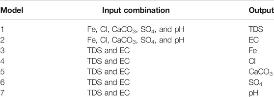
TABLE 2. Inputs and outputs of each modeling case.

Metrics Evaluation Models

Error values between calculated and observed data in this study are assessed via root mean square error (RMSE), mean absolute error (MAE), mean square error (MSE), coefficient of determination (R²) (Ighalo et al., 2021), and correlation coefficient (R) (Shabani et al., 2020):

$R=\frac{{{\displaystyle \sum }}_{i=1}^n(G_{\left(obs\right)i}-G_{\left(obs\right)})(G_{\left(pre\right)i}-G_{\left(pre\right)})}{\sqrt{{(G_{\left(obs\right)i}-G_{\left(obs\right)})}^2{{\displaystyle \sum }}_{i=1}^n{({\text{G}}_{\left(obs\right)}-G_{\left(obs\right)})}^2}},(16)$

${\text{R}}^2²=1-\frac{{{\displaystyle \sum }}_{i=1}^n{\left(G_{\left(obs\right)i}-{\displaystyle G_{\left(pre\right)i}}\right)}^2}{{{\displaystyle \sum }}_{i=1}^n{(G_{\left(obs\right)i}-G_{\left(obs\right)})}^2},(17)$

$RMSE=\sqrt{\frac{1}{\text{n}}{\displaystyle \sum }_{\text{i}=1}^{\text{n}}{\left(G_{\left(obs\right)i}-G_{\left(pre\right)i}\right)}^2},(18)$

$\text{MAE }=\frac{{{\displaystyle \sum }}_{i=1}^n\left|G_{\left(obs\right)i}-G_{\left(pre\right)i}\right|}{n},(19)$

$\text{MSE}=\frac{1}{\text{n}}{\displaystyle \sum }_{\text{i}=1}^{\text{n}}{\left(G_{\left(obs\right)i}-G_{\left(pre\right)i}\right)}^2,(20)$

where $G_{\left(obs\right)}$ and $G_{\left(pre\right)}$ represent the mean values of the groundwater quality observed and predicted, respectively, $G_{\left(obs\right)i}$ and $G_{\left(pre\right)i}$ are the observed and predicted, respectively, in the current original data $\left(i\right)$, and n is the number of samples. Figure 1 shows the method used in this study.

FIGURE 1

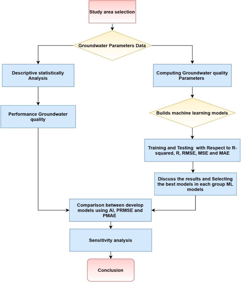
FIGURE 1. Flow diagram of the research study.

Results and Discussion

Machine Learning Model Performance

Linear regression models: In this section, training was conducted to estimate different kinds of multivariate LR models in the prediction of TDS, EC, Fe, Cl, SO₄, CaCO₃, and pH. To assess the performance of these models, R, R², RMSE, MAE, and MSE were calculated as displayed in Table 3. For developing the models, there is a need to split the collected data into training and testing data in order to create the optimal model architecture during training and examine model performance during testing. In order to split the collected data for training, validation, and testing, it is necessary to apply the trail-and-error procedure to search for the best splitting ration, which is long time-consuming to develop the model. Therefore, to avoid such a process, the data splitting built-in function has been utilized in order to automatically search for the optimal data splitting for training and testing data. In addition, for the validation data, the training data have been split automatically to training and validation data using the same function. So, the highest values of correlation coefficients are highlighted in bold font. Multivariate LR models were applied in the current study to predict the concentrations of Fe, Cl, SO₄, and CaCO₃ from measurements of TDS and EC. Various types of LR models (standard linear, stepwise, interactions, and robust regression) were used. Table 3 illustrates that the interaction regression model performs better than other models, such as standard linear, robust, and stepwise models, in predicting TDS, EC, Fe, Cl, CaCO₃, SO₄, and pH in terms of RMSE, with the lowest values of 158.22, 208.06, 4.5086, 28.467, 161.77, 217.06, and 0.55666, respectively. However, the MAE in the robust regression model was less than that in the interaction model in predicting Fe, CaCO₃, and SO₄ concentrations. From Table 3, all values of the coefficient of determination were better in the interaction regression model than in the other models, as shown in the bolded font. In addition, R², RMSE, MSE, and MAE are significant performance measurements, and consuming time in training is considered a significant metric to validate the quality of the model. Any model has less duration for training, and learning the parameters is considered better than others. In Table 3, in seven prediction models, standard linear regression models have the lowest time consumption in training compared to other models that have longer training times, except prediction of Cl and pH, and the stepwise regression model shows less time in training. However, the performance of multivariate linear regression for predicting only TDS and EC concentrations shows a moderate level of accuracy with R values of 0.6 and 0.7, respectively, while other groundwater parameter predictions demonstrate unacceptable performance.

TABLE 3

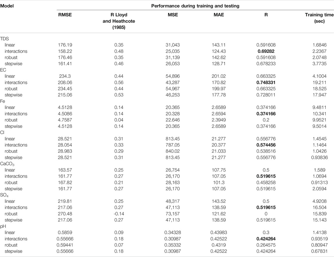
TABLE 3. Performance metrics of different types of LR models.

Tree Regression Models: For the TR learner model, fine, medium, and coarse trees were evaluated and compared in the training and tested phases, as demonstrated in Table 4, to predict parameters Fe, Cl, SO₄, pH, and CaCO₃ from measurements of TDS and EC. The hyperparameters of those models were tuned to optimize the models to provide better results. In Table 4, fine tree was capable of providing the best metrics in all input combinations compared to medium tree and coarse tree which were lesser precise in predicting all parameters of groundwater as highlighted in the bold font. The training speeds of the models are also compared in the last columns of the table. As is clear from Table 4, the fine tree performs superior to the others in all input combinations in terms of R more than 0.76, while the coarse tree provides the worst performance with R less than moderate accuracy. The best values of MAE and MSE were obtained from the fine tree model compared with the medium and coarse tree models. As expected, the fine tree also had the lowest RMSE values for TDS, EC, Fe, Cl, CaCO₃, SO₄, and pH at 96.458, 112.54, 3.1359, 22.035, 110.8, 126.54, and 0.30466, respectively. Coarse trees generally have the lowest training time, while fine trees may need a long duration for training (e.g., 17.332 s for predicting EC). It can be said that the increasing number of learners improves the model accuracy and that predicting EC generally produces the best accuracy. Generally, acceptable precision of the tree regression model performance is achieved by using a fine tree type. Additionally, among all groundwater prediction parameters, EC prediction achieved better performance, with the highest R² value of 0.87 compared with the other parameters predicted.

TABLE 4

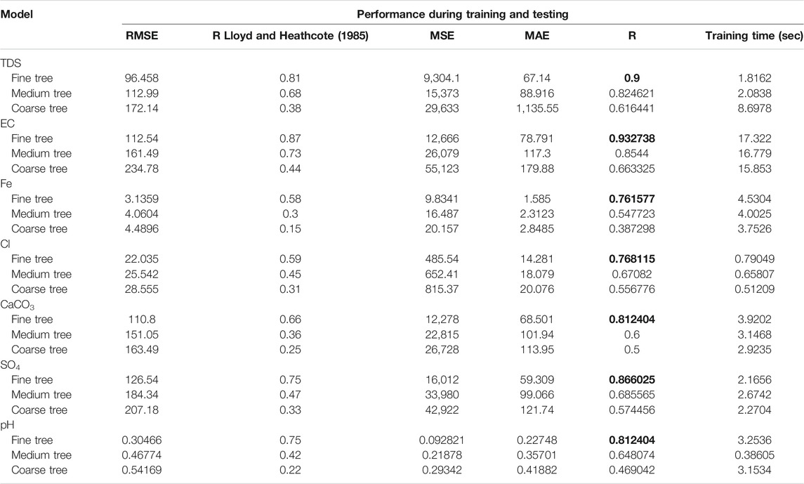
TABLE 4. Performances of the tree regression models.

Gaussian Process Regression Models: A comparison of different methods, such as squared exponential GPR, matern 5/2 GPR, rational quadratic GPR, and exponential GPR, clearly indicates that the exponential GPR model is superior to the other models. The best values of R² are highlighted in bold font in Table 5, which summarizes the performances of all models of the group GPR., The exponential GPR in all predictions of TDS, EC, Fe, Cl, CaCO₃, SO₄, and pH had lower RMSE values and the highest R² values with (76.104, 0.938083), (46.126, 0.989949), (3.9207, 0.591608), (24.073, 0.714143), (156.77, 0.556776), and (186.16, 0.678233) (0.42484, 0.72111), respectively. In addition, better values of MAE are provided by exponential GPR, compared with squared exponential GPR, matern 5/2 GPR, and rational quadratic GPR. On the other hand, the squared exponential GPR offered the worst accuracy with the worst values of MSE and MAE. Better accuracy of prediction gets for predicting EC, followed by TDS, with R more than 0.9; at the same time, outcomes of other predictions achieve acceptable range of accuracy with R more than 0.5. The rational quadratic GPR with most predictions can be considered good because it has lower training duration, while in prediction of SO₄, the exponential GPR has much lower training time with (2.8136 s) than rational quadratic GPR, squared exponential GPR, and matern 5/2 GPR with training time (15.145, 18.659, 17.263 s, which is considered another good alternative for exponential GPR. Overall, the GPR models show good performance in all groundwater parameters, with R starting from more than moderate (0.5) to more than 0.9 using various GPR methods.

TABLE 5

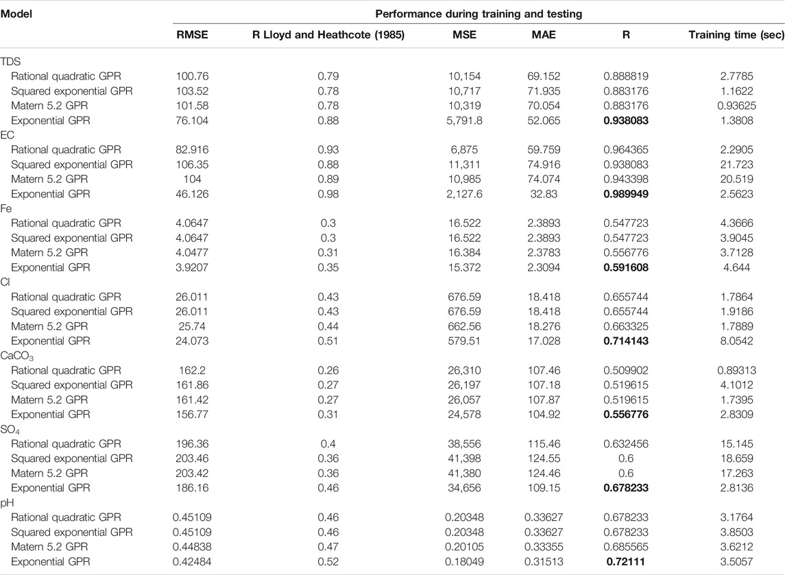
TABLE 5. Performances of the Gaussian process regression models.

Support vector regression models: In SVM models, different kernel functions were appraised for computation. These kernels are linear kernels, quadratic kernels, cubic kernels, and Gaussian or radial basis function (RBF) kernels that include three forms: fine, medium, and coarse. Among all kernels, fine kernel was able to give highest correlation coefficients in all prediction, except prediction of SO₄ concentration of groundwater, the cubic kernel showed better performance and achieved satisfactory accuracy with R more than 0.5. Additionally, the fine kernel produced better RMSE and MAE in predicting six out of seven parameters of groundwater TDS, EC, Fe, Cl, CaCO_3, and pH with values of (91.565, 50.364), (100.52, 61.03), (4.365, 1.9523), (25.349, 14.78), (157.83, 90.445), and (0.4266, 0.28639), respectively. In contrast, the cubic kernel gives the lowest RMSE and MAE in only the predicted SO₄ concentration, which has the best RMSE and MAE of 215.98 and 101.07, respectively, compared to the other kernels. Regarding training duration, it can be noticed from Table 6 that the best model fine Gaussian SVM displays less time training than linear, cubic, and quadratic medium and coarse at prediction of each of TDS, Fe, Cl concentrations with (0.62504, 2.0487, and 1.1556 s), respectively. Comparing between the results produced from prediction of each parameter of groundwater with others for best kernel that was selected, it can be said that better performance of the SVM model was attained in EC followed by TDS and pH concentrations in term coefficient of determination of 0.9, 0.83, and 0.52, respectively, while some predictions cannot achieve satisfactory range of accuracy, such as predict Fe concentration.

TABLE 6

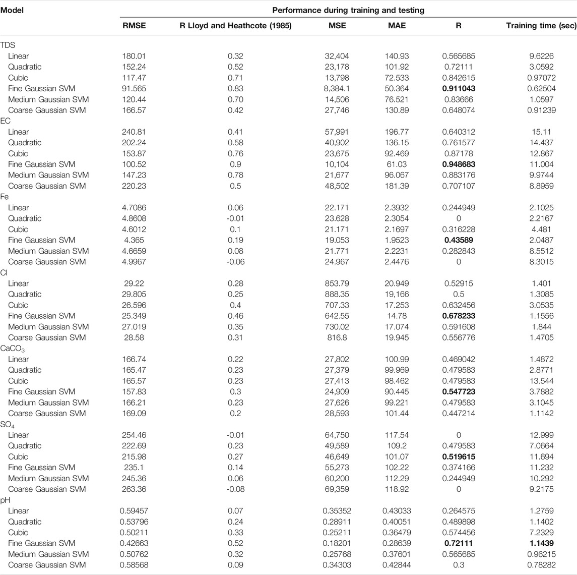
TABLE 6. Performances of the support vector machine models.

Ensemble Regression Models: As given in Table 7, the statistics of ensemble regression models are reported and compared in predicting groundwater concentrations for the training and testing stages. The models were optimized by tuning the hyperparameters to give the best results by adjusting each of the minimum leaf size, number of learners, and number of components. The superiority of the boosted tree ensemble over the bagged tree ensemble is apparent for all seven groundwater concentration predictions, as shown in bold font in Table 7. According to the boosted regression tree model, among all cases, the predicted EC had the highest coefficient of determination (0.96). The accuracy difference between the boosted tree and bagged tree shows positive influence of the boosted inputs in predicting groundwater concentrations; for example, in prediction of Cl, the improvement in MSE of the boosted tree is from (365.28–163.63) and in MAE from (13.12–7.94). Additionally, it could be concluded that both types of ensemble regression models provide good results in almost all predictions of groundwater parameters by reaching R greater than 0.8. With respect to time training, the Fe concentration prediction shows less time duration for boosted trees and bagged trees than other groundwater concentration prediction (1.4953 and 1.9125) seconds. For clarity, scatter plots will illustrate the prediction of the best model used in the prediction of every groundwater parameter, which is the boosted tree model, as in Figure 2.

TABLE 7

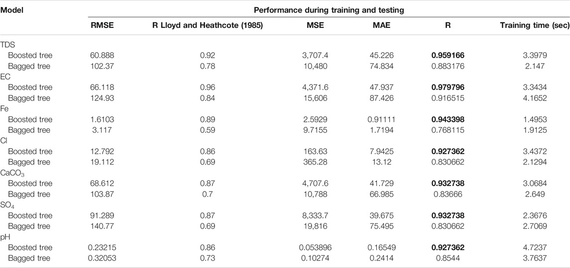
TABLE 7. Performances of the ensemble regression models.

FIGURE 2

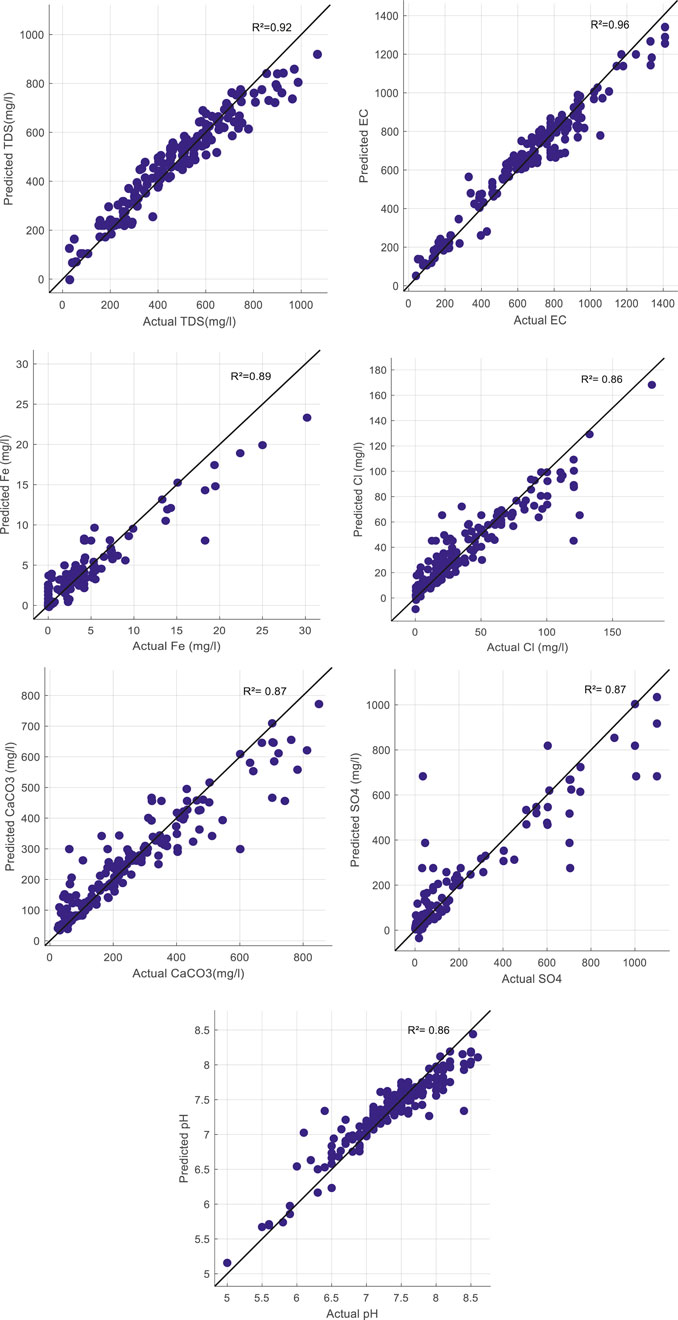
FIGURE 2. Scatter plot for observations and predictions using the boosted ensemble regression tree model to predict each groundwater quality parameter.

Predictive Models Comparison

A comparison of five regression models, including the interaction linear regression model (LR), fine tree regression model (TR), exponential Gaussian process regression (GPR), fine Gaussian support vector regression model (SVM), and boosted ensemble regression tree model (ER), is shown in Figure 3, Figure 4, and Figure 5 in terms of R, RMSE, and MAE, respectively. The first comparison was performed for seven groundwater parameters, including TDS, EC, Fe, Cl, CaCO₃, SO₄, and pH, using accuracy improvement (AI) from the equation below. Table 8 summarizes the best values of correlation coefficients for each group of models that were selected earlier, and the highest R is highlighted by bold font for each groundwater parameter.

$\text{AI}=\frac{{\text{R}}_{ER}- {\text{R}}_M}{{\text{R}}_{ER}}\times 100,(21)$

where ${\text{R}}_{ER}$ denotes the correlation coefficient of the model ER, whereas ${\text{R}}_M$ denotes a correlation coefficient for other models (LR, TR, GPR, and SVM). Figure 3 shows the model ranking based on AI in terms of R. The ensemble boosted tree model reveals excellent performance in six prediction parameters with remarkable positive accuracy improvement over TR 28% in TDS, 24% in EC, 60% in Fe, 40% in Cl, 44% in CaCO₃, 44% in SO₄, and 54% in pH. Additionally, it is clear that ER is more acceptable than TR, with significant improvements noted in prediction every case, which range from 5% to 19%. Predictive accuracy was significantly improved after presenting ER over GPR for six cases. Only in the case of EC did GPR demonstrate more satisfactory performance than ER, with slight improvement observed in AI with a negative value. Moreover, the findings show that ER not only displayed improved accuracy for certain parameters over LR, TR, and GPR but also this model has the capability to capture temporal patterns in groundwater parameters over SVM in all cases with meaningful improvements in predicting TDS, EC, Fe, Cl, CaCO₃, SO_4, and pH with 5%, 3%, 54%, 27%, 41%, 44%, and 22%, respectively. Generally, it can be concluded that the model ER exhibits high precision in all cases in terms of the correlation coefficients.

FIGURE 3

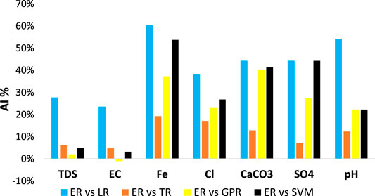
FIGURE 3. Accuracy improvement for the ER model over other models in terms of R.

FIGURE 4

FIGURE 4. Accuracy improvement for the ER model over other models in terms of RMSE.

FIGURE 5

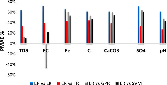
FIGURE 5. Accuracy improvement for the ER model over other models in terms of MAE.

TABLE 8

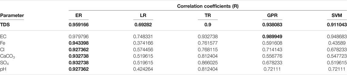
TABLE 8. Summary of correlation coefficients for the best five models.

Another analysis was performed to compare the models in predicting groundwater parameters. The improvement percentage of root mean squared errors (PRMSE) (MiweiLiu et al., 2017; Mi et al., 2019) RMSE must be reduced to obtain a robust model. Figure 4 illustrates the models ranking over the best model ER based on PRMSE. In prediction of TDS, the PRMSE for the boosted tree model over all models obtains a positive value, and GPR ranks as the second-best model in predicting the TDS parameter with a lesser percentage of 20%. On the other hand, in predicting the EC parameter, the ER model obtained a negative value over GPR of 43%, while over the other models, positive values were obtained. In such cases (Fe, Cl, CaCO₃, SO₄, and pH), the fine tree regression model TR ranked as the second-best model with the lowest PRMSE (49%, 42%, 38%, 28%, and 24%) compared with GPR and SVM. Furthermore, the LR model displays the worst outcomes with the highest PRMSE in all predictions of groundwater parameters, with 62% in TDS, 68% in EC, 64% in Fe, 54% in Cl, and 58% in CaCO₃, SO_4, and pH.

To compare the models in terms of MAE, the improvement percentage of mean absolute errors (PMAE) (MiweiLiu et al., 2017; Mi et al., 2019) was executed. Figure 5 shows that the highest PMAE was obtained for ER over LR in all cases, with 64% in TDS, 72% in EC, 66% in Fe, 71% in SO₄, and 61% in Cl, CaCO₃, and pH. It could be noticed in predicting TDS parameter that SVM ranked as a second-best model after boosted tree model with lesser PMAE: 10% compared with LR, TR, and GPR over the model ER, while in prediction of EC, the GPR shows higher performance over all models, including ER, which was had negative value with 46%. However, in the remaining predictions, the TR model ranked as the second-best model after the boosted tree model. Generally, it could be concluded that the boosted ensemble regression tree model exhibits high precision over all (LR, TR, GPR, and SVM) models with remarkable improvements in performance in terms of R, RMSE, and MAE.

The last comparison between models is in terms of duration consumed in training, and Figure 6 shows models ranked based on time consumed in training for seven groundwater quality parameters. One of the major benefits of ML models is that they consume little time in training. In cases of CaCO₃ and pH, the LR model was capable of decreasing the time of training compared with the GPR, ER, and SVM models, which took longer to train. On the other hand, the TR model takes less time of training in prediction of Cl and SO₄, with 0.79049 and 2.1656 s, respectively, than the LR model, which took the longest time in training. According to the GPR model, only one case shows less training time than the other models, which predicts EC within 2.5623 s. In general, the LR, TR, SVM, and GPR models have long training times in some cases, which can exceed 19, 17, 11, and 8 s in some cases, respectively, while the ensemble regression model (ER) was found to achieve such balance and performed better than the rest of the models in terms of training time and prediction error obtained via investigative attained R². The ER model revealed less training time in case of Fe, and the range of training time for the ER model in all cases was more reasonable than that of the rest of the models, which gives another advantage of the ER model.

FIGURE 6

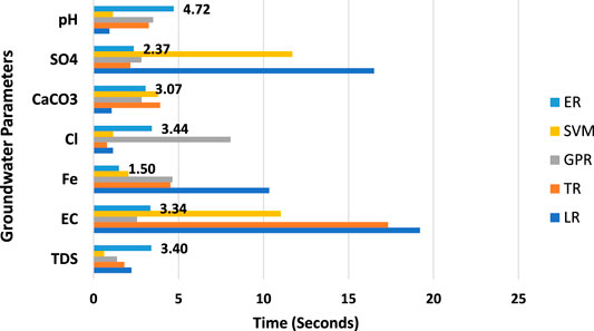
FIGURE 6. Comparison between models in terms of training time in prediction of groundwater parameters.

Sensitivity Analysis

With careful observation of the attained outcomes from the best model ER by considering the values of each performance indicator to assess model performance, additional outcomes can be elaborated. These analyses and elaboration may add a new direction for evaluating the performance of the selected model. To verify the potential prediction skill of the boosted tree model, the effect of each input parameter on the model’s performance against all parameters should be determined using performance indicators. From Table 9, it could be observed that in the case of removing pH and Fe parameters, there was no influence on boosted tree model performance, while in the prediction of TDS, the accuracies of the boosted tree model increased if any of the Cl or SO₄ parameters were eliminated with R² values of 0.93 and 0.94, respectively. Furthermore, the performance model has been influenced in improving the estimation efficiency by removing the CaCO₃ parameter because it caused a decrease in the R² values in both the predicted TDS and EC, so eliminating this groundwater parameter has the most significant impact on the performance of the boosted tree model.

TABLE 9

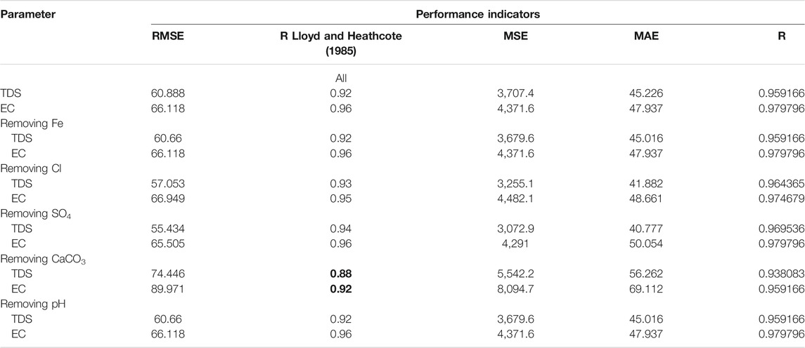
TABLE 9. Impact of removing input groundwater parameters on ER model performance for TDS and EC prediction.

At the end, it is worth mentioning that the comparison between the results of the current study and the results in study 20 in which same data were used shows that ensemble boosted regression tree model outperformed on artificial neural network (ANN) model. Figure 7 demonstrates the values of coefficient of determination for best models concluded from both studies, and it could be noticed that the R² values of the ER model ranged from 0.86 to 0.96, whereas for the ANN model, it ranged between 0.52 and 0.82 in prediction of each groundwater quality parameter.

FIGURE 7

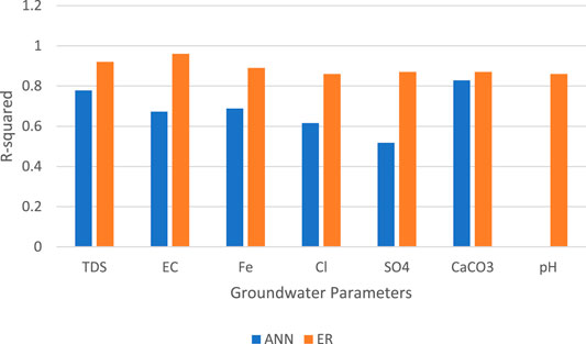
FIGURE 7. Comparison between the current study and that of Calvert, (2020) in terms of R² values.

Conclusion

In this study, various regression models with different architectures were developed by using hyperparameter optimization algorithms and compared to examine the application of groundwater concentration prediction. Evaluation metrics (R², RMSE, MSE, and MAE) were performed on all developed models to evaluate their performance. The outcomes of this study can be summarized as follows: In terms of accuracy, which is represented via R², each TR, GPR, and ER has satisfactory performance. The ER model attained superior accuracy in terms of R² in TDS 0.92, Fe 0.89, Cl 0.86, CaCO₃ 0.87, SO₄ 0.87, and pH 0.86 compared to all developed models. Moreover, relatively low training time was accomplished by the ER model. Comparisons between the developed models were performed using AI, PRMSE, and PMAE to measure the significance of the ER model over other developed models at each groundwater parameter. The findings showed that the ER model outperforms other machine learning models in predicting six parameters with remarkable percentages of AI, PRMSE, and PMAE. However, only electrical conductivity predictions with negative values were obtained for AI, PRMSE, and PMAE over the GPR model. Sensitivity analysis was conducted to determine the impact of the most significant variable on the prediction of TDS and EC using the best model selected. The results indicate that the total hardness parameter has the most influence on the accuracy of TDS and EC concentration predictions. In summary, ensemble regression models were found to balance high prediction accuracy in terms of R², low training time, and low errors in terms of RMSE and MAE. The limitation of this study is that the field of prediction of groundwater quality has been rapidly developed due to the fact that it provides obvious and compelling benefits for the management of water resources and environmental activities. Although the used datasets were comprehensive enough to accomplish the objectives of this study, but it could include collecting a bigger dataset from different hydrogeological settings for future research. Additionally, to analyze more data, research can also be performed with more ions and groundwater contaminants. For forthcoming studies, after obtaining additional datasets, recent deep learning models, such as 1D convolutional networks and long short-term memory, which were found to provide extraordinary performance in several applications, could be discovered in such applications of groundwater concentration prediction to be learning more hidden patterns that might contribute to increasing prediction precision.

Data Availability Statement

Publicly available datasets were analyzed in this study. These data can be found here: The data were used from a published study: Calvert, M. B. Predicting Concentrations of Selected ions and Total Hardness in Groundwater Using Artificial Neural Networks and Multiple Linear Regression Models (2020).

Author Contributions

Data curation: AMA and ANA; formal analysis: MSH, AR, and AMA; methodology: AHB and AE-S; writing—original draft: MSH and AMA; writing—review and editing: PK, MS, AS, and AE-S; funding: MS and AS.

Funding

The project was funded by UAE University with the initiatives of Asian Universities Alliance Collaboration.

Conflict of Interest

The authors declare that the research was conducted in the absence of any commercial or financial relationships that could be construed as a potential conflict of interest.

Publisher’s Note

All claims expressed in this article are solely those of the authors and do not necessarily represent those of their affiliated organizations, or those of the publisher, the editors, and the reviewers. Any product that may be evaluated in this article, or claim that may be made by its manufacturer, is not guaranteed or endorsed by the publisher.

References

Asefa, T., Kemblowski, M. W., Urroz, G., McKee, M., and Khalil, A. (2004). Support Vectors–Based Groundwater Head Observation Networks Design. Water Resour. Res. 40. doi:10.1029/2004wr003304

CrossRef Full Text | Google Scholar

Ayadi, A., Ghorbel, O., BenSalah, M. S., and Abid, M. (2019). A Framework of Monitoring Water Pipeline Techniques Based on Sensors Technologies. J. King Saud Univ. - Comput. Inf. Sci. 34, 47–57. doi:10.1016/j.jksuci.2019.12.003

CrossRef Full Text | Google Scholar

Basim, H. K., Mustafa, M. J., and Alsaqqar, A. S. (2018). Artificial Neural Network Model for the Prediction of Groundwater Quality. Int. J. Plant Soil Sci. 8, 1–13. doi:10.28991/cej-03091212

CrossRef Full Text | Google Scholar

Breiman, L. (1996). Bagging Predictors. Mach. Learn. 24, 123–140. doi:10.1007/bf00058655

CrossRef Full Text | Google Scholar

Breiman, L. (2001). Random Forests. Mach. Learn. 45, 5–32. doi:10.1023/a:1010933404324

CrossRef Full Text | Google Scholar

Calvert, M. B. (2020). Predicting Concentrations of Selected Ions and Total Hardness in Groundwater Using Artificial Neural Networks and Multiple Linear Regression Models North Carolina: Duke University in Durham.

Google Scholar

Castrillo, M., and García, Á. L. (2020). Estimation of High Frequency Nutrient Concentrations from Water Quality Surrogates Using Machine Learning Methods. Water Res. 172, 115490. doi:10.1016/j.watres.2020.115490

PubMed Abstract | CrossRef Full Text | Google Scholar

Chowdury, M. S. U., Emran, T. B., Ghosh, S., Pathak, A., Alam, M. M., Absar, N., et al. (2019). IoT Based Real-Time River Water Quality Monitoring System. Proced. Comput. Sci. 155, 161–168. doi:10.1016/j.procs.2019.08.025

CrossRef Full Text | Google Scholar

Crittenden, J. C., Trussell, R. R., Hand, D. W., Howe, K. J., and Tchobanoglous, G. (2012). MWH’s Water Treatment: Principles and Design. John Wiley & Sons.

Google Scholar

El Bilali, A., Taleb, A., and Brouziyne, Y. (2021a). Groundwater Quality Forecasting Using Machine Learning Algorithms for Irrigation Purposes. Agric. Water Manage. 245, 106625. doi:10.1016/j.agwat.2020.106625

CrossRef Full Text | Google Scholar

Elahi, E., Khalid, Z., Tauni, M. Z., Zhang, H., and Lirong, X. (2021b). Extreme Weather Events Risk to Crop-Production and the Adaptation of Innovative Management Strategies to Mitigate the Risk: A Retrospective Survey of Rural Punjab, Pakistan. Technovation, 102255. doi:10.1016/j.technovation.2021.102255

CrossRef Full Text | Google Scholar

Elahi, E., Khalid, Z., Weijun, C., and Zhang, H. (2020). The Public Policy of Agricultural Land Allotment to Agrarians and its Impact on Crop Productivity in Punjab Province of Pakistan. Land use policy 90, 104324. doi:10.1016/j.landusepol.2019.104324

CrossRef Full Text | Google Scholar

Elahi, E., Zhang, H., Lirong, X., Khalid, Z., and Xu, H. (2021). Understanding Cognitive and Socio-Psychological Factors Determining Farmers' Intentions to Use Improved Grassland: Implications of Land Use Policy for Sustainable Pasture Production. Land use policy 102, 105250. doi:10.1016/j.landusepol.2020.105250

CrossRef Full Text | Google Scholar

Elith, J., Leathwick, J. R., and Hastie, T. (2008). A Working Guide to Boosted Regression Trees. J. Anim. Ecol. 77, 802–813. doi:10.1111/j.1365-2656.2008.01390.x

CrossRef Full Text | Google Scholar

Freund, Y., and Schapire, R. E. (1996). Experiments with a New Boosting Algorithm. icml 96, 148–156.

Google Scholar

García, Á., Anjos, O., Iglesias, C., Pereira, H., Martínez, J., and Taboada, J. (2015). Prediction of Mechanical Strength of Cork under Compression Using Machine Learning Techniques. Mater. Des. 82, 304–311. doi:10.1016/j.matdes.2015.03.038

CrossRef Full Text | Google Scholar

Hastie, T., Tibshirani, R., and Friedman, J. (2009). The Elements of Statistical Learning: Data Mining, Inference, and Prediction New York, NY: Springer.

Google Scholar

Ighalo, J. O., Adeniyi, A. G., and Marques, G. (2021). Artificial Intelligence for Surface Water Quality Monitoring and Assessment: a Systematic Literature Analysis. Model. Earth Syst. Environ. 7, 669–681. doi:10.1007/s40808-020-01041-z

CrossRef Full Text | Google Scholar

Kecman, V. (2001). Learning and Soft Computing: Support Vector Machines, Neural Networks, and Fuzzy Logic Models. MIT press.

Google Scholar

Khalil, A., Almasri, M. N., McKee, M., and Kaluarachchi, J. J. (2005). Applicability of Statistical Learning Algorithms in Groundwater Quality Modeling. Water Resour. Res. 41, 1–16. doi:10.1029/2004wr003608

CrossRef Full Text | Google Scholar

Kim, D., Jeon, J., and Kim, D. (2019). Predictive Modeling of Pavement Damage Using Machine Learning and Big Data Processing. J. Korean Soc. Hazard. Mitig 19, 95–107. doi:10.9798/kosham.2019.19.1.95

CrossRef Full Text | Google Scholar

Kim, M. J., Yun, J. P., Yang, J. B. R., Choi, S. J., and Kim, D. (2020). Prediction of the Temperature of Liquid Aluminum and the Dissolved Hydrogen Content in Liquid Aluminum with a Machine Learning Approach. Metals (Basel). 10, 330. doi:10.3390/met10030330

CrossRef Full Text | Google Scholar

Knoll, L., Breuer, L., and Bach, M. (2017). Large Scale Prediction of Groundwater Nitrate Concentrations from Spatial Data Using Machine Learning. Sci. Total Environ. 668, 1317–1327. doi:10.1016/j.scitotenv.2019.03.045

CrossRef Full Text | Google Scholar

Kutner, M. H., Nachtsheim, C. J., Neter, J., and Li, W. (2005). Applied Linear Statistical Models, Vol. 5. McGraw-Hill Irwin Boston.

Google Scholar

Lloyd, J. W., and Heathcote, J. A. A. (1985). Natural Inorganic Hydrochemistry in Relation to Ground Water.

Google Scholar

Lu, H., and Ma, X. (2020). Hybrid Decision Tree-Based Machine Learning Models for Short-Term Water Quality Prediction. Chemosphere 249, 126169. doi:10.1016/j.chemosphere.2020.126169

PubMed Abstract | CrossRef Full Text | Google Scholar

Mi, X., Liu, H., and Li, Y. (2019). Wind Speed Prediction Model Using Singular Spectrum Analysis, Empirical Mode Decomposition and Convolutional Support Vector Machine. Energ. Convers. Manage. 180, 196–205. doi:10.1016/j.enconman.2018.11.006

CrossRef Full Text | Google Scholar

MiweiLiu, X.-w. H., Liu, H., and Li, Y.-f. (2017). Wind Speed Forecasting Method Using Wavelet, Extreme Learning Machine and Outlier Correction Algorithm. Energ. Convers. Manage. 151, 709–722. doi:10.1016/j.enconman.2017.09.034

CrossRef Full Text | Google Scholar

Mohamed, H., AbdelazimNegm, M., Salah, M., Nadaoka, K., and Zahran, M. (2017). Assessment of Proposed Approaches for Bathymetry Calculations Using Multispectral Satellite Images in Shallow Coastal/lake Areas: a Comparison of Five Models. Arab. J. Geosci. 10, 42. doi:10.1007/s12517-016-2803-1

CrossRef Full Text | Google Scholar

Mosavi, A., Hosseini, F. S., Choubin, B., Abdolshahnejad, M., Hamidreza, G., Lahijanzadeh, A., et al. (2020). Susceptibility Prediction of Groundwater Hardness Using Ensemble Machine Learning Models. Water 12 (10), 2770. doi:10.3390/w12102770

CrossRef Full Text | Google Scholar

World Health Organization (1993). Guidelines for Drinking-Water Quality Geneva, Switzerland: World Health Organization Press.

Google Scholar

Rajaee, T., Ebrahimi, H., and Nourani, V. (2019). A Review of the Artificial Intelligence Methods in Groundwater Level Modeling. J. Hydrol. 572, 336–351. doi:10.1016/j.jhydrol.2018.12.037

CrossRef Full Text | Google Scholar

Sain, S. R. (1996). The Nature of Statistical Learning Theory. Technometrics 38, 409. doi:10.1080/00401706.1996.10484565

CrossRef Full Text | Google Scholar

Schmoll, O., Howard, G., Chilton, J., and Chorus, I. (2006). Protecting Groundwater for Health: Managing the Quality of Drinking-Water Sources London, UK: IWA Publishing.

Google Scholar

Shabani, S., Samadianfard, S., Sattari, M. T., Mosavi, A., Shamshirband, S., Kmet, T., et al. (2020). Modeling pan Evaporation Using Gaussian Process Regression K-Nearest Neighbors Random Forest and Support Vector Machines; Comparative Analysis. Atmosphere (Basel). 11, 66. doi:10.3390/atmos11010066

CrossRef Full Text | Google Scholar

Shadrin, D., Nikitin, A., Tregubova, P., Terekhova, V., Jana, R., Matveev, S., et al. (2021). An Automated Approach to Groundwater Quality Monitoring—Geospatial Mapping Based on Combined Application of Gaussian Process Regression and Bayesian Information Criterion. Water 13, 400. doi:10.3390/w13040400

CrossRef Full Text | Google Scholar

Singha, S., Pasupuleti, S., Singha, S. S., Singh, R., and Kumar, S. (2021). Prediction of Groundwater Quality Using Efficient Machine Learning Technique. Chemosphere 276, 130265. doi:10.1016/j.chemosphere.2021.130265

PubMed Abstract | CrossRef Full Text | Google Scholar

TiyashaTung, T. M., Tung, T. M., and Yaseen, Z. M. (2020). A Survey on River Water Quality Modelling Using Artificial Intelligence Models: 2000-2020. J. Hydrol. 585, 124670. doi:10.1016/j.jhydrol.2020.124670

CrossRef Full Text | Google Scholar

Vijay, S., and Kamaraj, K. (2019). Ground Water Quality Prediction Using Machine Learning Algorithms in R. Int. J. Res. Anal. Rev. 6, 743–749.

Google Scholar