Feasibility of Random Forest and Multivariate Adaptive Regression Splines for Predicting Long-Term Mean Monthly Dew Point Temperature

The accurate estimation of dew point temperature (T_dew) is important in climatological, agricultural, and agronomical studies. In this study, the feasibility of two soft computing methods, random forest (RF) and multivariate adaptive regression splines (MARS), is evaluated for predicting the long-term mean monthly T_dew. Various weather variables including air temperature, sunshine duration, relative humidity, and incoming solar radiation from 50 weather stations in Iran as well as their geographical information (or a subset of them) are used in RF and MARS as inputs. Three statistical indicators namely, root mean square error (RMSE), mean absolute error (MAE), and correlation coefficient (R) are used to assess the accuracy of T_dew estimates from both models for different input configurations. The results demonstrate the capability of the RF and MARS methods for predicting the long-term mean monthly T_dew. The combined scenarios in both the RF and MARS methods are found to produce the best T_dew estimates. The best T_dew estimates were obtained by the MARS model with the RMSE, MAE, and R of respectively 0.17°C, 0.14°C, and 1.000 in the training phase; 0.15°C, 0.12°C, and 1.000 in the validation phase; and 0.18°C, 0.14°C, and 0.999 in the testing phase.

Introduction

Dew point temperature (T_dew) is defined as the temperature (at constant pressure) in which water vapor in the air condenses into liquid water. The accurate estimation of T_dew is required in many fields such as climatology, hydrology, meteorology, and agronomy (Emmel et al., 2010; Millán et al., 2010; Katul et al., 2012; Feld et al., 2013; Mohammadi et al., 2015; Mohammadi et al., 2016; Alizamir et al., 2020a). T_dew along with the wet bulb temperature can be used to compute ambient temperature (Snyder and Melo-Abreu, 2005; Shank, 2006; Mohammadi et al., 2016). The dew point also allows plants to adapt themselves for possible frosts (Mohammadi et al., 2016). T_dew is an essential element for plant survival, particularly in regions with low precipitation (Agam and Berliner, 2006). T_dew is necessary for estimating relative humidity and evapotranspiration (Hubbard et al., 2003). Robinson (2000) stated that T_dew is important for assessing long-term climate variability.

In recent years, soft computing and data mining approaches have been widely employed as powerful techniques for predicting T_dew. A review of the literature shows that random forest (RF) and multivariate adaptive regression splines (MARS) methods have rarely been utilized to estimate T_dew; however, they have been extensively used for predicting other hydro-climatological variables (Heddam et al., 2020; Kisi et al., 2021; Tan et al., 2021).

Shank et al. (2008) predicted T_dew at 20 weather stations in Georgia by using weather data into artificial neural networks (ANN). It was found that ANN could reliably predict T_dew. Zounemat-Kermasni (2012) predicted hourly T_dew data via the ANN and multiple linear regression (MLR) approaches. Kisi et al. (2013) evaluated the robustness of generalized regression neural networks (GRNN), Kohonen self-organizing feature maps (KSOFM), and adaptive neuro-fuzzy inference system (ANFIS) for estimating T_dew at the Daegu, Pohang, and Ulsan stations in South Korea. The accuracy of GRNN and ANFIS were similar and better than that of KSOFM. Shiri et al. (2014) estimated daily T_dew data at two weather stations in the Republic of Korea using gene expression programming (GEP) and ANN models. Various combinations of climatic variables were used as inputs, with the accuracy of GEP was found to be higher than that of ANN. Kim et al. (2015) investigated the potential of multi-layer perceptron (MLP), GRNN, and MLR in estimating daily T_dew at two weather stations in California. They defined different combinations of weather data as model predictors. The results indicated that the T_dew estimates from GRNN were better than those of MLP. Mohammadi et al. (2015) evaluated the accuracy of the extreme learning machine (ELM), ANN, and support vector machine (SVM) approaches in predicting daily T_dew at Bandar Abbas and Tabas, Iran. The mean air temperature, relative humidity, atmospheric pressure, solar radiation, and vapor pressure were used as model inputs. The results revealed that ELM and ANN produced the best and worst daily T_dew estimates, respectively. Amirmojahedi et al. (2016) utilized a coupled model by combining ELM with wavelet transform (WT) for predicting daily T_dew in Bandar Abbas, South Iran. The accuracies of hybrid ELM-WT and single ELM were compared with those of SVM and ANN. Four different input scenarios were used in their models. Mohammadi et al. (2016) estimated daily T_dew at two stations in Iran by the ANFIS technique. Different ANFIS models were developed using various input combinations. Their results demonstrated that water vapor pressure was the most influential variable for the accurate prediction of T_dew. Mehdizadeh et al. (2017a) employed GEP to estimate daily T_dew at the Urmia and Tabriz stations in Northwest Iran. Various input scenarios were developed using meteorological variables and lagged T_dew data. Moreover, T_dew at each station was predicted using data from a nearby station. Qasem et al. (2019) estimated daily T_dew at the Tabriz station in Iran using GEP, SVM, and M5 model tree (M5), with M5 was found to show the highest performance. Naganna et al. (2019) attempted to increase the accuracy of estimating T_dew at two stations in India by coupling the MLP with two bio-inspired optimization algorithms. The hybrid methods outperformed the classic MLP. Alizamir et al. (2020b) recommended a deep echo state network (DESN) to forecast daily T_dew at two locations in the Republic of Korea. The proposed model produced the best performance compared to other soft computing methods. Dong et al. (2020) improved the performance of ELM by optimization algorithms to estimate daily T_dew in Yangling, China. They indicated the better accuracy of hybrid models compared to the classic ELM.

Given the importance of T_dew in various disciplines, particularly agriculture and hydrology, its precise prediction is vital. Therefore, this study investigated the applicability of random forest (RF) and multivariate adaptive regression splines (MARS) for predicting the long-Temperature-, sunshine duration-, radiation-, other climatic variables-, geographical information-, and combined-based input scenarios were considered in this study.

Only a few studies used RF and MARS to predict T_dew (Shiri, 2018). Also, the correct choice of inputs for soft computing models plays an important role in achieving their optimal performance. Hence, this study attempted to find the best input combination.

Materials and Methods

Study Region and Data

The study area was Iran, which is located in southwest Asia. With an area of about 1,648,000 km², Iran spans over the latitude of25°00 N′- 40°00 N′ and longitude of 44°00′ E-63°30′ E. The locations of the study stations are shown in Figure 1. Table 1 presents the geographical properties of the selected stations. As can be seen in Table 1, the long-term mean annual T_dew ranges from -2.58 °C at Kerman to 20.70 °C at Chabahar.

FIGURE 1

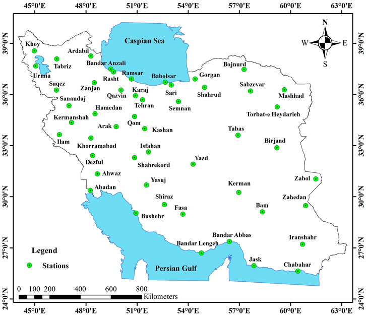
FIGURE 1. Spatial distribution of the studied stations in Iran.

TABLE 1

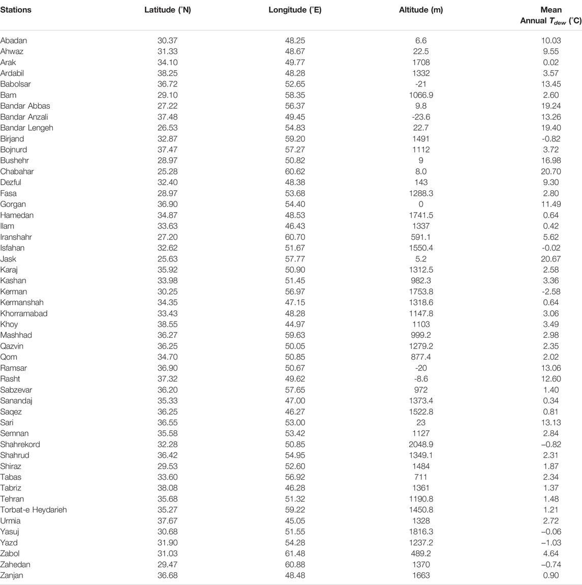
TABLE 1. Geographical properties of the stations in Iran and long-term mean annual values of T_dew.

Meteorological data from 50 stations (compiled by the Iran Meteorological Organization, IMO) were utilized in this study. The data include long-term mean monthly dew point temperature (T_dew), minimum, maximum, and mean air temperatures (T_min, T_max, T), solar radiation (R_s), sunshine duration (S), relative humidity (RH), vapor pressure (V_p), and precipitation (P) between 1951 and 2015. Statistical characteristics of these variables are presented in Table 2. In this table, S_o and R_a denote the maximum possible sunshine duration and extraterrestrial radiation, respectively, which were calculated based on the relationships presented by Allen et al. (1998). La, Lo and Alt are the latitude, longitude, and altitude of study stations, respectively. We can observe that T_min, S_o, R_a and V_p respectively in the temperature-sunshine duration- radiation- and other meteorological variables-based input scenarios have the highest correlations with T_dew (Table 2). Figure 2 illustrates the long-term mean monthly of meteorological variables in the study stations.

TABLE 2

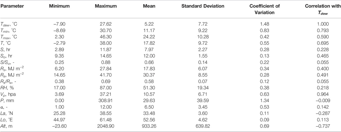
TABLE 2. Statistical characteristics of long-term mean monthly meteorological data.

FIGURE 2

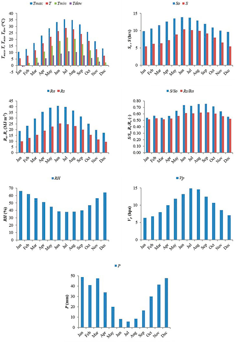
FIGURE 2. Long-term mean monthly meteorological variables in the study stations.

The data were split into three parts. 70% (420 months), 15% (90 months), and 15% (months) of the data were used for training, testing, and validating the models, respectively.

Random Forest

Random forest (RF), first developed by Breiman (2001), is a powerful ensemble learning algorithm. This model can be employed for regression, classification, and unsupervised learning problems (Liaw and Wiener, 2002). Many decision trees are created using the RF technique via permutation and continual variation of the elements influencing the intended parameter, before all created trees are incorporated for the prediction. Over-fitting, which may occur in the decision tree approach, is eliminated when the number of trees increases. Hence, at every phase of tree growth, the developed model becomes more accurate, and the error rate is reduced. In the RF, the bagging process is utilized to choose random samples of variables as the training dataset. Next, for each variable, if the values of that variable are permuted across the out-of-bag observations, the function specifies the model prediction error (Trigila et al., 2015). Various bootstrap samples of the data, a sampling approach with permutations, were involved in the construction of the RF. Therefore, some out-of-bag datasets were generated from the training dataset via the repetition of the sampling operation.

The number of trees is the most important feature affecting the accuracy of RF (Breiman, 2001). The optimal number of trees is determined by trial and error. 500 trees were used in the RF as increasing the number of trees did not improve its performance.

Multivariate Adaptive Regression Splines

Multivariate adaptive regression splines (MARS) were initially presented by Friedman (1991). This is a non-parametric regression technique, in which the response/target variable can be estimated by using a series of coefficients and functions called basis functions. Cheng and Cao (2014) stated that one of the advantages of MARS is its ability to estimate the contributions of these basis functions. Therefore, the additive and interactive influences of input predictors are allowed to specify the target variable.

The typical form of a MARS model can be defined as follows:

$y=f\left(x\right)=c_o+{\displaystyle \sum _{i=1}^m{c}_i{b}_i\left(x\right)}(1)$

where y is the dependent variable predicted by MARS, x is the independent variable(s), c_o is a primary constant or bias, c_i is the coefficient for the ith basis function, and b_i(x) indicates the ith basis function.

The MARS model consists of two phases: forward and backward. The prediction process begins using an intercept, which is the average of the dependent parameter values. The basis functions are subsequently added continuously to the developed model. It should be noted that when the basis functions are added, the model considers the functions that cause a significant reduction in the sum of square errors. In the forward stage, an over-fitted MARS that include a large number of knots is realized. Then, the backwards stage prunes the model until a suitable MARS is presented based on the lowest value for the generalized cross-validation criterion.

Performance Investigation Metrics

The accuracies of the models were evaluated using three statistical metric: root mean square error (RMSE), mean absolute error (MAE), and correlation coefficient (R). These metrics can be expressed as follows:

$RMSE=\sqrt{\frac{{\displaystyle {\sum }_{i=1}^N{\left(T_{o,i}-T_{p,i}\right)}^2}}{N}}(2)$

$MAE=\frac{1}{N}{\displaystyle \sum _{i=1}^N\left|T_{o,i}-T_{p,i}\right|}(3)$

$R=\frac{{\displaystyle {\sum }_{i=1}^N\left(T_{o,i}-\overline{T_o}\right)\left(T_{p,i}-\overline{T_p}\right)}}{\sqrt{\left[{\displaystyle {\sum }_{i=1}^N{\left(T_{o,i}-\overline{T_o}\right)}^2}\right]\left[{\displaystyle {\sum }_{i=1}^N{\left(T_{p,i}-\overline{T_p}\right)}^2}\right]}}(4)$

where T_o,i and T_p,i are the ith measured and predicted long-term mean monthly T_dew, respectively; $\overline{T_o}$ and $\overline{T_p}$ denote the mean of the measured and predicted values of the long-term mean monthly T_dew, respectively, and N is the number of data points.

Low values for the RMSE and MAE indices, and a high value of the R index indicate higher performance of the model for predicting the long-term mean monthly T_dew.

Results and Discussion

This study evaluated the performance of two soft computing approaches, RF and MARS, for predicting the long-term mean monthly T_dew at 50 stations in Iran. Thirty-one scenarios in six categories were considered to identify the most important variables affecting T_dew, and to determine the best input combinations. The RMSE, MAE, and R values were employed to assess the accuracy of the methods.

Performance of RF and MARS Approaches

The statistical indices of dew point estimates from the RF and MARS approaches for various input scenarios are presented in Tables 3, 4, respectively.

TABLE 3

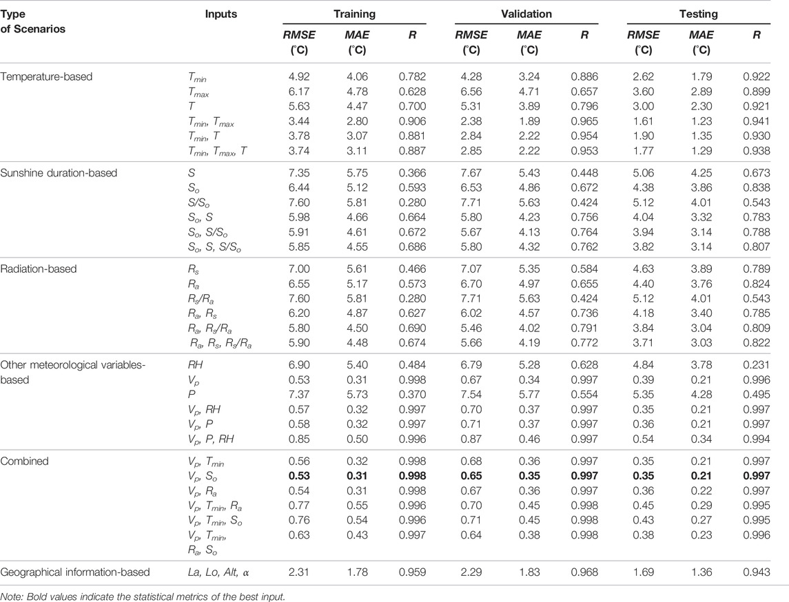
TABLE 3. Statistical indices of T_dew estimates from the RF model for the training, validation, and testing phases.

TABLE 4

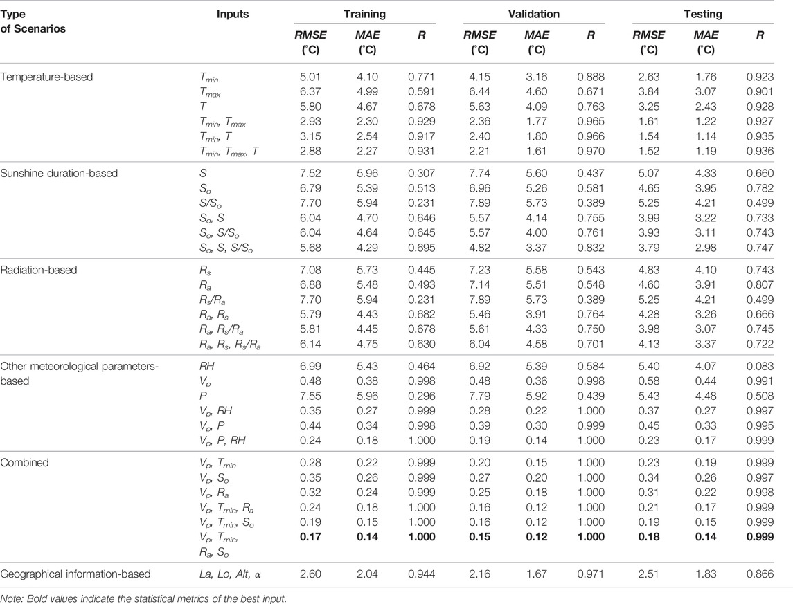
TABLE 4. Statistical indices of T_dew estimates from the MARS model for training, validation, and testing phases.

In the temperature-based input scenarios, T_min and T both produced better results than T_max., T_dew was found to have a higher correlation with T_min than T and T_max. Therefore, better results were obtained by employing T_min as the input. The superiority of T_min compared to T and T_max was also found by Mohammadi et al. (2016) and Mehdizadeh et al. (2017a). T_dew is more correlated with T_min as cool air cannot retain water vapor much longer, meaning the effect of T_min on T_dew is greater than those of T_max and T (Mehdizadeh et al., 2017a). To develop scenarios with more inputs, T and T_max were added to T_min. A similar strategy was followed to develop scenarios with multiple inputs for other categories. The input combination of T_min and T_max exhibited a better accuracy than T_min and T. Also, the scenarios with all inputs generally yielded better results in comparison with the scenarios with fewer inputs, particularly single-input scenarios. Air temperature is typically measured at all weather stations. Therefore, it can be easily used as a possible input predictor to predict T_dew.

Among the sunshine duration-based scenarios, S_o and S/S_o were the best and the worst predictors, respectively. Input combinations S_o and S, and S_o and S/S_o generally produced a similar accuracy, particularly for the MARS model. Interestingly, the S_o and S/S_o scenario was slightly better than the S_o and S scenario in the RF approach. The full-input scenario performed best in both the RF and MARS approaches. However, the performance of this scenario is still not accurate enough for predicting T_dew. Additionally, a sunshine duration sensor is needed to measure the sunny hours, which may not be available at some locations. Therefore, the application of sunshine duration variables as the only input of the models is not recommended.

In the radiation-based scenarios, the input R_a showed the best accuracy, while the performance of the clearness index (R_s/R_a) was not as good as R_s. In general, the performance of the R_a and R_s/R_a input combinations was slightly better than that of R_a and R_s single-input predictors. The RF approach generally produced the highest accuracy with the full-input scenario in the radiation-based classes. However, for the MARS models, two-input scenarios exhibited better performance than the full-input scenario. Similar to the sunshine duration scenarios, radiation-based input combinations did not perform satisfactorily, resulting in higher values of RMSE and MAE and lower values of R. Solar radiation is measured by pyranometer, a relatively expensive device that may not be available at weather stations in developing countries. Therefore, the use of radiation-based scenarios may be limited.

In the other meteorological scenarios, various combinations of RH, V_p, and P were examined. The results for the single-input scenarios show that V_p is the most influential input variable for the accurate prediction of T_dew. Also, the performance of this predictor is better than the most effective variables in temperature- (i.e., T_min), sunshine duration- (i.e., S_o), and radiation-based (i.e., R_a) scenarios. For the V_p predictor, the RMSE, MAE, and R of T_dew estimates from the RF method in the testing phase were 0.39°C, 0.21°C, and 0.996, respectively. Corresponding values from the MARS method were0.58°C, 0.44°C and 0.991. Furthermore, the model with RH as input performed better than P. Comparing the statistical indices of single RH and P scenarios with the two- and full-input scenarios shows that the accuracy of T_dew predictions significantly increased by adding V_p to RH and P. For the two-input and three-input scenarios, the Vp and RH combination in the RF method, and the Vp, P, and RH combination in the MARS method were the best performers.

The most important variables of the four classes (i.e., T_min, S_o, R_a, and V_p) were employed to develop the combined scenarios. The performance of T_min, S_o, and R_a was not as good as that of V_p. However, the feasibility of T_min, S_o, and R_a was considerably improved by adding V_p into them. In the combined-based classes with two inputs, V_p and T_min in the MARS model, and V_p and S_o in the RF model yielded slightly better T_dew estimates. Interestingly, utilizing three-input and four-input scenarios did not necessarily increase the accuracy of the RF method. But, the accuracy of the MARS method was enhanced by increasing the number of predictors. All combined scenarios produced reliable results due to the higher R values and lower RMSE and MAE values. Unfortunately, these scenarios require many weather variables, which is typically unavailable in developing countries. These scenarios can only be used to predict T_dew at weather stations, which are able to measure all required meteorological parameters.

The long-term mean monthly T_dew can also be predicted from the geographical characteristics (i.e., latitude, longitude, and altitude) and periodicity (α), which denotes the number of months (i.e., one for January and 12 for December). These predictors can be applied to predict the long-term mean monthly T_dew without using meteorological data. These results support the outcomes of previous studies (Kisi et al., 2015; Kisi and Sanikhani, 2015; Mehdizadeh et al., 2017b; Sanikhani et al., 2018) in which the geographical information and number of month were successfully utilized in soft computing models to predict mean monthly time series of hydrological variables such as air and soil temperatures, precipitation, and reference evapotranspiration.

As can be seen in Tables 3, 4, T_min, S_o, R_a, and V_p variables showed more accurate results than the other sole-input scenarios. The better performance of these predictors in their respective scenario classes can be attributed to their high correlations with T_dew (see Table 2).

Comparison of MARS and RF Approaches for Different Input Scenarios

It can be concluded that the RF method is generally superior to the MARS method for the single-input temperature-, sunshine duration-, and radiation-based scenarios. However, the MARS approach generally showed a better performance for the multi-input scenarios. The geographical information-based scenario was superior in the RF method compared to the MARS method. In contrast, the other weather variable-based classes (except the single RH and single P inputs, and the combined scenarios) performed better in MARS than RF.

Comparison of predicted and measured long-term mean monthly T_dew values by the best inputs for the training, validation, and testing phases are depicted in Figure 3. As can be seen in Figure 3, these inputs can accurately predict long-term mean monthly T_dew. As shown in Tables 3, 4, the input combination of V_p and S_o in the RF approach, and V_p, T_min, R_a, and S_o in the MARS model were the superior combinations in all of the three study periods (bold text in Tables 3, 4). The estimates of long-term mean monthly T_dew using these inputs are very close to the measured data, particularly for the MARS method.

FIGURE 3

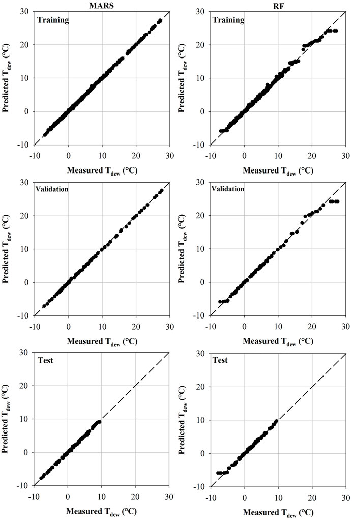
FIGURE 3. Dew point temperature (T_dew) predicted by the superior scenarios of RF and MARS approaches versus the measured values for the training, validation, and test phases.

The results revealed that the other weather variable-based (except the single RH and single P variables) and combined scenarios outperformed the other scenarios (Table … … ). However, for both methods, combined scenarios indicated a slightly better performance over other weather variables-based scenarios. Temperature-based combinations had better performance compared to sunshine duration- and radiation-based scenarios, which both had the lowest prediction accuracies. Furthermore, the accuracy of the geographical information-based combinations was better than the temperature-, sunshine duration-, and radiation-based scenarios. This confirms the feasibility of RF and MARS for predicting the long-term mean monthly T_dew from the geographical information and the periodicity term.

Conclusion

This study evaluated the performance of two soft computing approaches, random forest (RF) and multivariate adaptive regression splines (MARS), for predicting the long-term mean monthly T_dew. To specify the influential variables, different input combinations consisting of meteorological variables, geographical characteristics, and the periodicity component were employed as inputs in the RF and MARS models. The meteorological variables included minimum, maximum, and mean air temperatures (T_min, T_max, and T); actual sunshine duration, maximum possible sunshine duration, and sunshine duration ratio (S, S_o, and S/S_o); actual solar radiation, extraterrestrial radiation, and clearness index (R_s, R_a, and R_s/R_a); and relative humidity (RH), vapor pressure (V_p), and precipitation (P). Thirty-one input scenarios were considered in six different categories: temperature-, sunshine duration-, radiation-, other weather variable-, geographical information-based, and combined scenarios. The results obtained are summarized as follows:

• For the single-input scenarios, T_min, S_o, R_a, and V_p were the optimum inputs for the temperature-, sunshine duration-, radiation-, and other weather variables r-based scenarios, respectively. Among these variables, V_p had the best performance.

• sunshine duration- and radiation-based scenarios showed the lowest accuracy, while the combined scenarios performed the best.

• The geographical information-based scenarios were superior to the temperature-, sunshine duration-, and radiation-based scenarios. Therefore, the geographical properties and periodicity term can be used to predict the long-term mean monthly T_dew without using any meteorological data.

• In general, the single-input scenarios had a higher accuracy for the RF model compared to the MARS model. While, the multi-input scenarios in the MARS model outperformed the RF method.

• The best multi-input combinations were V_p and S_o for RF, and V_p, T_min, R_a and S_o for MARS.

• V_p can be used as the sole input in both the RF and MARS approaches to predict the long-term mean monthly T_dew with acceptable accuracy.

Often only a few input configurations were used to estimate different hydrologic variables such as evaporation, solar radiation, soil temperature. The various inputs scenarios used in this study can be tested in future works to find the best input combinations for estimating different variables of interest. Other standalone and coupled models can be used in future studies to estimate T_dew and compare it with the outcomes of this work.

Data Availability Statement

The original contributions presented in the study are included in the article/Supplementary Material, further inquiries can be directed to the corresponding author.

Author Contributions

All the authors listed have made a substantial, direct, and intellectual contribution to the work and approved it for publication.

Conflict of Interest

The authors declare that the research was conducted in the absence of any commercial or financial relationships that could be construed as a potential conflict of interest.

Publisher’s Note

All claims expressed in this article are solely those of the authors and do not necessarily represent those of their affiliated organizations, or those of the publisher, the editors and the reviewers. Any product that may be evaluated in this article, or claim that may be made by its manufacturer, is not guaranteed or endorsed by the publisher.

References

Agam, N., and Berliner, P. R. (2006). Dew Formation and Water Vapor Adsorption in Semi-arid Environments-A Review. J. Arid Environments 65 (4), 572–590. doi:10.1016/j.jaridenv.2005.09.004

CrossRef Full Text | Google Scholar

Alizamir, M., Kim, S., Zounemat-Kermani, M., Heddam, S., Kim, N. W., and Singh, V. P. (2020a). Kernel Extreme Learning Machine: an Efficient Model for Estimating Daily Dew point Temperature Using Weather Data. Water 12 (9), 2600. doi:10.3390/w12092600

CrossRef Full Text | Google Scholar

Alizamir, M., Kim, S., Kisi, O., and Zounemat-Kermani, M. (2020b). Deep echo State Network: a Novel Machine Learning Approach to Model Dew point Temperature Using Meteorological Variables. Hydrological Sci. J. 65 (7), 1173–1190. doi:10.1080/02626667.2020.1735639

CrossRef Full Text | Google Scholar

Allen, R. G., Pereira, L. S., Raes, D., and Smith, M. (1998). Crop Evapotranspiration. GuideLines for Computing Crop Evapotranspiration. Rome, Italy: FAO Irrigation and Drainage Paper No. 56.

Google Scholar

Amirmojahedi, M., Mohammadi, K., Shamshirband, S., Seyed Danesh, A., Mostafaeipour, A., and Kamsin, A. (2016). A Hybrid Computational Intelligence Method for Predicting Dew point Temperature. Environ. Earth Sci. 75, 1–12. doi:10.1007/s12665-015-5135-7

CrossRef Full Text | Google Scholar

Breiman, L. (2001). Random Forests. Mach. Learn. 45, 5–32. doi:10.1023/a:1010933404324

CrossRef Full Text | Google Scholar

Cheng, M.-Y., and Cao, M.-T. (2014). Accurately Predicting Building Energy Performance Using Evolutionary Multivariate Adaptive Regression Splines. Appl. Soft Comput. 22, 178–188. doi:10.1016/j.asoc.2014.05.015

CrossRef Full Text | Google Scholar

Dong, J., Wu, L., Liu, X., Li, Z., Gao, Y., Zhang, Y., et al. (2020). Estimation of Daily Dew point Temperature by Using Bat Algorithm Optimization Based Extreme Learning Machine. Appl. Therm. Eng. 165, 114569. doi:10.1016/j.applthermaleng.2019.114569

CrossRef Full Text | Google Scholar

Emmel, C., Knippertz, P., and Schulz, O. (2010). Climatology of Convective Density Currents in the Southern Foothills of the Atlas Mountains. J. Geophys. Res. 115 (D11). doi:10.1029/2009jd012863

CrossRef Full Text | Google Scholar

Feld, S. I., Cristea, N. C., and Lundquist, J. D. (2013). Representing Atmospheric Moisture Content along Mountain Slopes: Examination Using Distributed Sensors in the Sierra Nevada, California. Water Resour. Res. 49 (7), 4424–4441. doi:10.1002/wrcr.20318

CrossRef Full Text | Google Scholar

Friedman, J. H. (1991). Multivariate Adaptive Regression Splines. Ann. Statist. 19, 1–67. doi:10.1214/aos/1176347963

CrossRef Full Text | Google Scholar

Heddam, S., Ptak, M., and Zhu, S. (2020). Modelling of Daily lake Surface Water Temperature from Air Temperature: Extremely Randomized Trees (ERT) versus Air2Water, MARS, M5Tree, RF and MLPNN. J. Hydrol. 588, 125130. doi:10.1016/j.jhydrol.2020.125130

CrossRef Full Text | Google Scholar

Hubbard, K. G., Mahmood, R., and Carlson, C. (2003). Estimating Daily Dew point Temperature for the Northern Great Plains Using Maximum and Minimum Temperature. Agron. J. 95 (2), 323–328. doi:10.2134/agronj2003.0323

CrossRef Full Text | Google Scholar

Katul, G. G., Oren, R., Manzoni, S., Higgins, C., and Parlange, M. B. (2012). Evapotranspiration: a Process Driving Mass Transport and Energy Exchange in the Soil-Plant-Atmosphere-Climate System. Rev. Geophys. 50 (3). doi:10.1029/2011RG000366

CrossRef Full Text | Google Scholar

Kim, S., Singh, V. P., Lee, C.-J., and Seo, Y. (2015). Modeling the Physical Dynamics of Daily Dew point Temperature Using Soft Computing Techniques. KSCE J. Civ Eng. 19 (6), 1930–1940. doi:10.1007/s12205-014-1197-4

CrossRef Full Text | Google Scholar

Kisi, O., Kim, S., and Shiri, J. (2013). Estimation of Dew point Temperature Using Neuro-Fuzzy and Neural Network Techniques. Theor. Appl. Climatol. 114 (3-4), 365–373. doi:10.1007/s00704-013-0845-9

CrossRef Full Text | Google Scholar

Kisi, O., Sanikhani, H., Zounemat-Kermani, M., and Niazi, F. (2015). Long-term Monthly Evapotranspiration Modeling by Several Data-Driven Methods without Climatic Data. Comput. Elect. Agric. 115, 66–77. doi:10.1016/j.compag.2015.04.015

CrossRef Full Text | Google Scholar

Kisi, O., Khosravinia, P., Heddam, S., Karimi, B., and Karimi, N. (2021). Modeling Wetting Front Redistribution of Drip Irrigation Systems Using a New Machine Learning Method: Adaptive Neuro- Fuzzy System Improved by Hybrid Particle Swarm Optimization - Gravity Search Algorithm. Agric. Water Manag. 256, 107067. doi:10.1016/j.agwat.2021.107067

CrossRef Full Text | Google Scholar

Kisi, O., and Sanikhani, H. (2015). Prediction of Long-Term Monthly Precipitation Using Several Soft Computing Methods without Climatic Data. Int. J. Climatol. 35 (14), 4139–4150. doi:10.1002/joc.4273

CrossRef Full Text | Google Scholar

Liaw, A., and Wiener, M. (2002). Classification and Regression by Random forest. R. News 2 (3), 18–22.

Google Scholar

Mehdizadeh, S., Behmanesh, J., and Khalili, K. (2017a). Application of Gene Expression Programming to Predict Daily Dew point Temperature. Appl. Therm. Eng. 112, 1097–1107. doi:10.1016/j.applthermaleng.2016.10.181

CrossRef Full Text | Google Scholar

Mehdizadeh, S., Behmanesh, J., and Khalili, K. (2017b). Evaluating the Performance of Artificial Intelligence Methods for Estimation of Monthly Mean Soil Temperature without Using Meteorological Data. Environ. Earth Sci. 76, 1–16. doi:10.1007/s12665-017-6607-8

CrossRef Full Text | Google Scholar

Millán, H., Ghanbarian-Alavijeh, B., and García-Fornaris, I. (2010). Nonlinear Dynamics of Mean Daily Temperature and Dewpoint Time Series at Babolsar, Iran, 1961-2005. Atmos. Res. 98, 89–101. doi:10.1016/j.atmosres.2010.06.001

CrossRef Full Text | Google Scholar

Mohammadi, K., Shamshirband, S., Motamedi, S., Petković, D., Hashim, R., and Gocic, M. (2015). Extreme Learning Machine Based Prediction of Daily Dew point Temperature. Comput. Elect. Agric. 117, 214–225. doi:10.1016/j.compag.2015.08.008

CrossRef Full Text | Google Scholar

Mohammadi, K., Shamshirband, S., Petković, D., Yee, P. L., and Mansor, Z. (2016). Using ANFIS for Selection of More Relevant Parameters to Predict Dew point Temperature. Appl. Therm. Eng. 96, 311–319. doi:10.1016/j.applthermaleng.2015.11.081

CrossRef Full Text | Google Scholar

Naganna, S. R., Deka, P. C., Ghorbani, M. A., Biazar, S. M., Al-Ansari, N., and Yaseen, Z. M. (2019). Dew point Temperature Estimation: Application of Artificial Intelligence Model Integrated with Nature-Inspired Optimization Algorithms. Water 11 (4), 742. doi:10.3390/w11040742

CrossRef Full Text | Google Scholar

Qasem, S. N., Samadianfard, S., Nahand, H. S., Mosavi, A., shamshirband, S., and Chau, K.-w. (2019). Estimating Daily Dew point Temperature Using Machine Learning Algorithms. Water 11 (3), 582. doi:10.3390/w11030582

CrossRef Full Text | Google Scholar

Robinson, P. J. (2000). Temporal Trends in United States Dew point Temperatures. Int. J. Climatol. 20 (9), 985–1002. doi:10.1002/1097-0088(200007)20:9<985::aid-joc513>3.0.co;2-w

CrossRef Full Text | Google Scholar

Sanikhani, H., Deo, R. C., Samui, P., Kisi, O., Mert, C., Mirabbasi, R., et al. (2018). Survey of Different Data-Intelligent Modeling Strategies for Forecasting Air Temperature Using Geographic Information as Model Predictors. Comput. Elect. Agric. 152, 242–260. doi:10.1016/j.compag.2018.07.008

CrossRef Full Text | Google Scholar

Shank, D. B. (2006). Dew point Temperature Prediction Using Artificial Neural Networks. MS thesis. United Kingdom: Harding University.

Google Scholar

Shank, D. B., Hoogenboom, G., and McClendon, R. W. (2008). Dewpoint Temperature Prediction Using Artificial Neural Networks. J. Appl. Meteorol. Climatol. 47 (6), 1757–1769. doi:10.1175/2007jamc1693.1

CrossRef Full Text | Google Scholar

Shiri, J., Kim, S., and Kisi, O. (2014). Estimation of Daily Dew point Temperature Using Genetic Programming and Neural Networks Approaches. Hydrol. Res. 45 (2), 165–181. doi:10.2166/nh.2013.229

CrossRef Full Text | Google Scholar

Shiri, J. (2018). Prediction vs. Estimation of Dewpoint Temperature: Assessing GEP, MARS and RF Models. Hydrol. Res. 50 (2), 633–643. doi:10.2166/nh.2018.104

CrossRef Full Text | Google Scholar

Snyder, R. L., and Melo-Abreu, J. P. D. (2005). Frost Protection: Fundamentals, Practice and Economics, 1. Rome: Food and Agricultural Organization of the United Nations.

Google Scholar

Tan, J., Xie, X., Zuo, J., Xing, X., Liu, B., Xia, Q., et al. (2021). Coupling Random forest and Inverse Distance Weighting to Generate Climate Surfaces of Precipitation and Temperature with Multiple-Covariates. J. Hydrol. 598, 126270. doi:10.1016/j.jhydrol.2021.126270

CrossRef Full Text | Google Scholar

Trigila, A., Iadanza, C., Esposito, C., and Scarascia-Mugnozza, G. (2015). Comparison of Logistic Regression and Random Forests Techniques for Shallow Landslide Susceptibility Assessment in Giampilieri (NE Sicily, Italy). Geomorphology 249, 119–136. doi:10.1016/j.geomorph.2015.06.001

CrossRef Full Text | Google Scholar

Zounemat-Kermasni, M. (2012). Hourly Predictive Levenberg–Marquardt ANN and Multi Linear Regression Models for Predicting of Dew point Temperature. Meteorol. Atmos. Phys. 117, 181–192. doi:10.1007/s00703-012-0192-x

CrossRef Full Text | Google Scholar

Nomenclature

T_dew Dew point temperature

MARS Multivariate adaptive regression splines

RF Random forest

ANN Artificial neural networks

MLR Multiple linear regression

GRNN Generalized regression neural networks

KSOFM Kohonen self-organizing feature maps

ANFIS Adaptive neuro-fuzzy inference system

GEP Gene expression programming

MLP Multi-layer perceptron

ELM Extreme learning machine

SVM Support vector machine

WT Wavelet transform

M5 M5 model tree

DESN Deep echo state network

T_min Minimum air temperature

T_max Maximum air temperature

T Mean air temperature

S sunshine duration

S_o Maximum possible sunshine duration

R_s Solar radiation

R_a Extraterrestrial radiation

RH Relative humidity

V_p Vapor pressure

P Precipitation

La Latitude

Lo Longitude

Alt Altitude

y Dependent variable predicted using the MARS

x Independent variable in MARS

c_o Bias

c_i Coefficient for the ith basis function of the MARS

b_i(x) ith basis function

RMSE Root mean square error

MAE Mean absolute error

R Correlation coefficient

T_o,i ith measured long-term mean monthly T_dew

T_p,i ith predicted long-term mean monthly T_dew

$\overline{{\mathrm{T}}_{\mathrm{o}}}$ Mean of the measured values of the long-term mean monthly T_dew

$\overline{{\mathrm{T}}_{\mathrm{p}}}$ Mean of the predicted values of the long-term mean monthly T_dew