A New Technique to Quantify the Local Predictability of Extreme Events: The Backward Nonlinear Local Lyapunov Exponent Method

Extreme weather events have a large impact on society, but are challenging to forecast accurately. In this study, we carried out a theoretical investigation of the local predictability of extreme weather events using the Lorenz model. We introduce a new method using the backward nonlinear local Lyapunov exponent to quantitatively estimate the local predictability limits of extreme events. The local predictability limits of extreme events on an individual orbit of a dynamical trajectory are broadly the same, whereas this is not the case if they are on different orbits. The specific structure of the Lorenz attractor is responsible for this phenomenon. Our results show that the local predictability limits of extreme events do not decrease or increase monotonically as the events increase in magnitude. This indicates that the magnitude of extreme events is not the only factor that affects the local predictability. The dynamical flow, initial error size, and structure of an attractor may also affect the local predictability. We also quantitatively compared the local predictability of extreme warm and cold events. This showed that the local predictability limits of extreme warm events are higher than extreme cold events at the same probability. A statistical analysis (i.e., the minimum, first quartile, median, third quartile, and maximum) also suggests that the extreme warm events have higher local predictability limits. In general, extreme warm events are more predictable than extreme cold events.

Introduction

Extreme weather events have significant economic and societal impacts (Laaidi et al., 2012; Howe et al., 2019; Sun et al., 2019). Numerous studies have shown that the frequency and intensity of extreme weather events increase due to global warming (Dosio et al., 2018; Howe et al., 2019; Nayak and Takemi, 2019). As such, it is increasingly important to be able to accurately forecast extreme events, although this remains challenging. The forecasting skills of extreme events need to be improved. The chaotic nature of atmospheric systems and relatively poor predictability of numerical models contribute to the low forecasting skill. In addition, insufficient data mean that the physical mechanisms of extreme events are poorly understood. Consequently, forecasting extreme events is an important field of current research.

Since the concept of predictability was proposed by Thompson (1957) and Lorenz (1963), a number of studies have investigated atmospheric predictability, including extreme events. Hallerberg et al. (2007) used the receiver operating characteristic (ROC) curve to investigate the predictability of extreme increments in an auto-regressive model with an order of one for wind speed and long-range correlated data. The results showed that the predictability increases as the size of the events increases, which is consistent with some previous studies (Lamper et al., 2001; Göber et al., 2004; Kantz et al., 2004). Hallerberg and Kantz (2008a) further investigated under what circumstances large events are more predictable than smaller events. They found that the predictability of different sized events follows a probability distribution function (PDF). If the PDF of the underlying stochastic process is Gaussian, then larger events have a higher predictability, whereas they have lower predictability if the PDF has a power-law tail. In the case of an exponential distribution, the predictability is not significantly associated with the event size. However, Hallerberg and Kantz (2008b) found that the predictability of large events is better for all types of distributions. Franzke (2012) used reduced order models to study the predictability of extreme events and showed that larger events are more predictable. Bódai (2015) used the ROC curve to study the predictability of larger extreme events with a low-order model and demonstrated that larger events are more predictable when there are no model errors. Although the aforementioned studies suggest that extreme events have a higher predictability, some studies have indicated this is not the case. Sterk et al. (2012) used the finite-time Lyapunov exponent (FTLE, e.g., Nese, 1989; Yoden and Nomura, 1993) method to investigate the predictability of extreme values in three different geophysical models. Sterk et al. (2012) showed that the observable attractors of dynamical systems and the prediction lead time all affect the predictability of extreme values. However, it was not possible to determine whether extreme or non-extreme events were more predictable without specific scenarios. Subsequently, Sterk et al. (2016) investigated if the predictability decreases as the extreme events become larger. Using the mean-squared error (MSE) and daily wind speed forecasts produced by an ensemble prediction system it was shown that the predictability decreases for larger extreme events. Sterk and Kekem (2017) further demonstrated that the predictability of extreme events depends on the dynamical model regime and does not have universal properties.

Based on the aforementioned studies, it is clear that the predictability of extreme events is complex and requires development of a robust method to assess the predictability. The FTLE method used by Sterk et al. (2012) characterized the average growth rate of infinitesimally small errors in a linear regime. However, the initial errors related to extreme events in real atmospheric systems may have a finite size. In addition, the initial errors increase nonlinearly because of the chaotic nature of the atmosphere (Mu and Duan, 2003; Mu et al., 2007; Duan and Mu, 2009). As such, the FTLE method may not be suitable for studying the predictability of extreme events. Based on the nonlinear local Lyapunov exponent (NLLE, e.g., Ding and Li, 2007; Ding et al., 2008; Li et al., 2020b)method (e.g., Ding and Li, 2007; Ding et al., 2008; Li et al., 2020a), we recently developed a new method, which is the backward nonlinear local Lyapunov exponent (BNLLE) method (Li et al., 2019; Li et al., 2020a; Li et al., 2021). The BNLLE method takes into account nonlinearity, and can be used to study the predictability of given states and, in particular, extreme states. This method can determine how far in the future it is possible to predict an extreme event before it happens. Unlike the NLLE method, it continuously searches backwards for the corresponding initial state of an extreme state. When the corresponding initial state is found, the time length between the corresponding initial state and extreme state is determined as the predictability limit of the extreme state.

The objective of this research was to apply the BNLLE method to study the local predictability of extreme events in a theoretical model. The local predictability limits (LPLs) of extreme events were quantitatively estimated with the BNLLE method. In addition, we assessed what types of extreme (i.e., warm and cold) events are more predictable. The remainder of this paper is structured as follows. Section Data, Dynamical Model and Methodology introduces data, the theoretical model and BNLLE method. Section Definitions of Extreme Warm and Cold Events describes the definitions of extreme events, and how extreme warm and cold events can be identified. Quantitative estimates and a comparison of the local predictability of extreme warm and cold events are described in Section Results. Finally, Section Discussion and Conclusion discusses our results and provides some conclusions based on our research.

Data, Dynamical Model and Methodology

Data

The time series of variables x, y, and z in the Lorenz model are obtained by integrating from the model. Besides, we also applied the BNLLE method to estimating the predictability of an extreme heatwave event occurring in European in June of 2019. The forecasts of surface (2 m) temperature are from the TIGGE (THORPEX Interactive Grand Global Ensemble) dataset with a horizontal resolution of 0.5° × 0.5° (Bougeault et al., 2010; Swinbank et al., 2016). The forecasts are made every day at 00/06/12/18Z on each start day, and the forecast time range is up to 15 days. There are total 51 ensemble members (one control forecast and 50 perturbed forecasts). The observed surface (2 m) temperature is from ERA-interim analysis dataset on a 0.5° grid (Dee et al., 2011). The ERA-interim data is four times a day (00/06/12/18Z). Based on the TIGGE and ERA-interim datasets, the error growths can be calculated, then they are used in analysis for quantifying the predictability of the heatwave event.

Lorenz63 Model

Lorenz (1963) designed a simplified model (hereafter Lorenz63) to study predictability. The Lorenz63 model can be used as a weather model, with only warm and cold regimes (Evans et al., 2004). It has some dynamical properties consistent with the real atmospheric system (Palmer, 1993; Goodliff et al., 2020). In addition, the Lorenz63 model is simple, which is beneficial for performing a large number of numerical simulations at relatively low computational cost. Therefore, the Lorenz63 model was used in this study. The dynamical equations are as follows:

$\{\begin{array}{c}\dot{x}=-\sigma \left(x-y\right)\\ \dot{y}=-xz+rx-y\\ \dot{z}=xy-bz\end{array}.(1)$

where $\sigma ,r$, and $b$ are three parameters. In this study, they are 10, 28, and 8/3, respectively. In this scenario, the model exhibits chaos.

The Lorenz63 model was integrated for 50,000 time steps using the fourth-order Runge–Kutta scheme with a time step of 0.01 time units (tus). The first 10,000 time states were for the spin-up and discarded. The remaining 40,000 states were used for our analysis.

The Backward Nonlinear Local Lyapunov Exponent Method

For a dynamical system, the predictability is associated with the growth rate of initial errors perturbed on an initial condition. The growth of initial errors can be described by:

$\mathit{\delta }\left({\mathit{t}}_{\text{0}}+\tau \right)=\mathit{\eta }\left(\mathit{x}\left({\mathit{t}}_{\text{0}}\right),\mathit{\delta }\left({\mathit{t}}_{\text{0}}\right),\tau \right)\mathit{\delta }\left({\mathit{t}}_{\text{0}}\right),(2)$

where $\mathit{\delta }\left({\mathit{t}}_{\text{0}}\right)$ and $\mathit{\delta }\left({\mathit{t}}_{\text{0}}+\tau \right)$ represent the initial errors and errors at time ${\mathit{t}}_{\text{0}}+\tau$. $\mathit{\eta }\left(\mathit{x}\left({\mathit{t}}_{\text{0}}\right),\mathit{\delta }\left({\mathit{t}}_{\text{0}}\right),\tau \right)$ is the nonlinear error propagation term that propagates the initial errors $\mathit{\delta }\left({\mathit{t}}_{\text{0}}\right)$ forward to $\mathit{\delta }\left({\mathit{t}}_{\text{0}}+\tau \right)$. This differs from previous studies (Vallejo and Sanjuan, 2013; Nastac et al., 2017; Vannitsem, 2017) in which the initial errors were assumed to be infinitesimally small and to increase in a linear regime. To measure the average nonlinear growth rate of errors over a finite time interval, Ding and Li (2007) proposed a new concept, the nonlinear local Lyapunov exponent (NLLE), which is expressed as:

$\mathbf{\lambda }\left(\text{x}\left({\text{t}}_{\text{0}}\right)\text{,}\mathit{\delta }\left({\text{t}}_{\text{0}}\right)\text{,τ}\right)=\frac{1}{\text{τ}}\text{ln}\frac{\Vert \mathit{\delta }\left({\text{t}}_{\text{0}}+\text{τ}\right)\Vert }{\Vert \mathit{\delta }\left({\text{t}}_{\text{0}}\right)\Vert },(3)$

where $\mathit{\lambda }\left(\mathit{x}\left({\mathit{t}}_{\text{0}}\right),\mathit{\delta }\left({\mathit{t}}_{\text{0}}\right),\tau \right)$ is the NLLE that measures the average nonlinear growth rate of the errors. It depends on the initial condition $\mathit{x}\left({\mathit{t}}_{\text{0}}\right)$, initial errors $\mathit{\delta }\left({\mathit{t}}_{\text{0}}\right)$, and integration time. For a number of initial errors perturbed on the same initial condition, the ensemble mean NLLE can be given by:

$\overline{\text{λ}}\left(\text{x}\left({\text{t}}_{\text{0}}\right),\mathit{\delta }\left({\text{t}}_{\text{0}}\right),\tau \right)={\langle {\mathit{\lambda }}_{\mathit{i}}\left(\text{x}\left({\text{t}}_{\text{0}}\right),\mathit{\delta }\left({\text{t}}_{\text{0}}\right),\tau \right)\rangle }_{\text{n}},(4)$

where ${\langle \rangle }_{\text{n}}$ represents the average of samples with a large size N $\left(\text{N}\to \infty \right)$. The mean relative growth of the initial error (RGIE) can be obtained from:

$\overline{\text{E}}\left(\text{x}\left({\text{t}}_{\text{0}}\right)\text{,}\mathit{\delta }\left({\text{t}}_{\text{0}}\right)\text{,τ}\right)=\text{exp}\left(\overline{\text{λ}}\left(\text{x}\left({\text{t}}_{\text{0}}\right)\text{,}\mathit{\delta }\left({\text{t}}_{\text{0}}\right)\text{,τ}\right)\text{τ}\right).(5)$

Based on Ding and Li (2007), the evolution of the RGIE from an initial condition $\mathit{x}\left({\mathit{t}}_{\text{0}}\right)$ can be described by:

$\overline{\text{E}}\left(\text{x}\left({\text{t}}_{\text{0}}\right)\text{,}\mathit{\delta }\left({\text{t}}_{\text{0}}\right)\text{,τ}\right)\stackrel{p}{\to }c,(6)$

where $\stackrel{p}{\to }$ denotes the convergence in the probability and c is a constant that RGIE converges to. The constant c can be considered to represent the climatology. When the RGIE reaches c, the information regarding the initial condition $\mathit{x}\left({\mathit{t}}_{\text{0}}\right)$ is lost, meaning the predictability is also lost. Therefore, the local predictability of the initial condition $\mathit{x}\left({\mathit{t}}_{\text{0}}\right)$ can be quantitatively determined as being the time from the initial time to the climatology time. Figure 1 shows an example of the NLLE and RGIE as a function of the time steps in the Lorenz63 model. The initial state is (−3.87, −5.69, 18.01), and its LPL is approximately 11 tus. The LPL is the longest prediction time from the initial state. However, what is important is the prediction lead time for extreme events. The NLLE method cannot estimate the prediction lead time of extreme events. In order to estimate the prediction lead time of extreme events, Li et al. (2019) developed the NLLE method and proposed the BNLLE method.

FIGURE 1

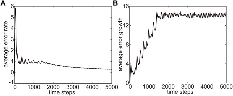
FIGURE 1. Variations of the average error (A) rate and (B) growth as a function of time. The initial state and error in the Lorenz63 model are (−3.87, −5.69, 18.01) and 10⁻⁵, respectively.

The BNLLE method firstly takes the extreme state $x\left({\text{t}}_{ex}\right)$ as a target state. We then search backwards for the corresponding initial state $x\left({\text{t}}_{in}\right)$ from previous states. It should be noted that:

$t_{in}<t_{ex}.(7)$

The corresponding initial state $x\left({\text{t}}_{in}\right)$ should meet the condition that the RGIE from it will converge to the constant c at the extreme state $x\left({\text{t}}_{ex}\right)$. When a state meets this condition, it is the corresponding initial state of the extreme state. In search of the corresponding initial states, the situation that multiple states meet the condition may happen. In this case, we always choose a state that maximizes the prediction lead time of the extreme state, as the corresponding initial state (Li et al., 2019). Therefore, the LPL of the extreme state $x\left({\text{t}}_{ex}\right)$ can be quantitatively estimated as:

$\text{LPT}=t_{\mathit{ex}}-t_{in}.(8)$

Definitions of Extreme Warm and Cold Events

The Lorenz63 attractor has warm and cold regimes, which can be considered to represent warm and cold weather (Evans et al., 2004). For the warm regime, the variables x and y should satisfy the following conditions:

$\{\begin{array}{c}x>0\\ y>0\end{array},(9)$

whereas, for the cold regime, the variables x and y should satisfy the following conditions:

$\{\begin{array}{c}x<0\\ y<0\end{array}.(10)$

We chose 40,000 consecutive events on the Lorenz attractor. For the warm regime, there were 17,292 warm events. For the cold regime, there were 18,534 cold events. The other 4,174 events are in the transitional regime, which neither belong to warm nor cold events. We then adopted the relative threshold method to define the extreme warm and cold events. The local predictabilities of the first component x of the Lorenz63 model were examined in this study. If an event x exceeds the 90th percentile of all the warm events, then this event x is an extreme warm event. Similarly, if an event x is lower than the 10th percentile of all the cold events, then this event x is an extreme cold event. It should be pointed out that the Lorenz63 model is quite simple, and lack of physical processes, compared with the actual atmosphere. In the model, there are no extreme high or low temperature processes corresponding to the real atmosphere. Thus, we call extreme warm and cold events instead of extreme high or low temperature in the study. Figure 2 shows the spatial distribution of extreme warm and cold events. The extreme warm and cold events are all distributed on the edges of the Lorenz attractor.

FIGURE 2

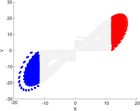
FIGURE 2. Spatial distribution of the extreme warm and cold events on the Lorenz attractor projected onto the x–y plane. Red and blue solid dots represent extreme warm and cold events, respectively. Gray solid dots represent normal warm and cold events.

Results

Local Predictability of Extreme Events

In this study, for each event, we randomly generated 10,000 different initial error vectors, which have the same magnitudes (10⁻⁵), but in different directions. The initial error vectors were then superimposed on each state. Based on the BNLLE method, the LPLs of the extreme warm and cold events can be quantitatively estimated. Figure 3 shows the spatial distribution of the LPLs of the extreme warm and cold events. For both the warm and cold regimes, the LPLs of the events on different orbits of a dynamical trajectory are different, whereas they are similar for the same orbit of a dynamical trajectory (i.e., the LPLs exhibit an obvious layered structure). Li et al. (2020a) noted that this phenomenon is determined by the specific structure of the Lorenz attractor. The events on an individual orbit around the center of either regime may have similar dynamical properties, which leads to similar LPLs. Different LPLs for events on different orbits result from the varying dynamical properties of the different orbits.

FIGURE 3

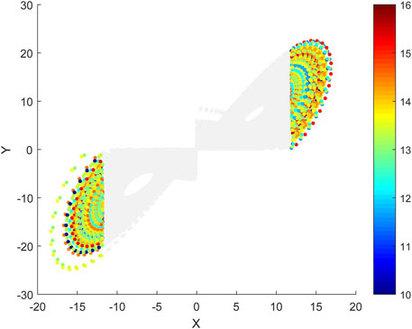
FIGURE 3. Spatial distribution of the LPLs of the extreme warm and cold events.

The minimum LPL is ∼10 tus, and the maximum is ∼16 tus (Figure 3). As such, the LPLs of the extreme events are highly variable. To further examine the distribution structure of the LPLs of extreme events, the extreme warm and cold events were classified based on percentile thresholds. Figure 4 is a box-and-whisker plot of the LPLs of extreme warm events and their standard deviations. For the 93rd to 97th percentiles, the maximum values are higher than the other percentiles (>16 tus), whereas their minimum values are lower than the other percentiles. For the 91st to 96th percentiles, the standard deviations of the LPLs are high. However, the standard deviations of the LPLs decrease from the 97th to 98th percentiles. The standard deviation of the LPLs for the 99th percentile increases again, and reaches a maximum. Figure 5 shows the box-and-whisker plot and standard deviations for the extreme cold events. For the 7th to 9th percentiles, the LPLs have larger maximum values and lower minimum values than the other percentiles. The maximum and minimum standard deviations of the LPLs are for the 4th and 2nd percentiles, respectively. The standard deviations of the 6th to 9th percentiles are broadly the same.

FIGURE 4

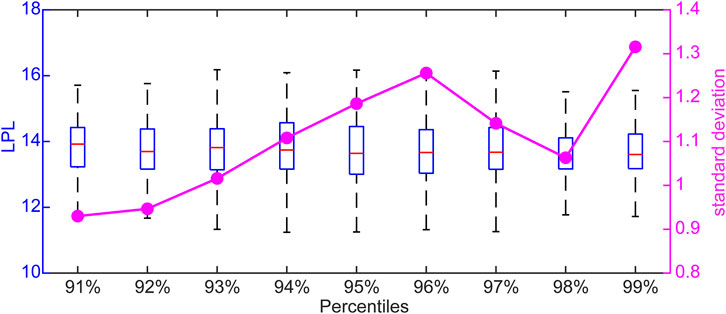
FIGURE 4. Box-and-whisker plot of the LPLs of extreme warm events in different percentiles. The pink symbols and line represent the standard deviations.

FIGURE 5

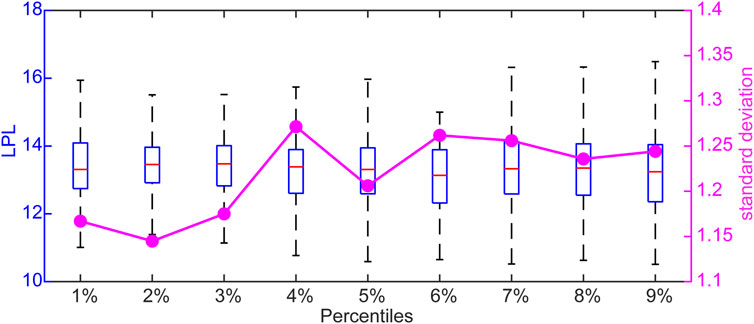
FIGURE 5. Same as for Figure 4, but for extreme cold events.

We use the term spread here to represent the standard deviation. For a group of extreme events with the same magnitude, a larger spread of LPLs results from different dynamical properties of the extreme events. This indicates that it is not easy to forecast these extreme events in this group. If the LPLs have a small spread, then these extreme events have similar dynamical properties, which would probably lead to good forecasts. Therefore, the spread can qualitatively reflect the average predictability of events in a group. The spread of the LPLs of the two types of extreme events does not decrease or increase monotonically as the magnitude of the extreme events increases (Figures 4, 5). This suggests that the magnitude of extreme events is not the only factor that affects predictability. In addition to the magnitude, the spatial position of the dynamical flow, error size, and structure of the Lorenz attractor all affect the LPLs of the extreme events.

From the above results, the BNLLE method can estimate the predictability of extreme events in the Lorenz model. To further verify the feasibility of the method, we also applied the BNLLE method to quantify the predictability of an extreme heatwave event in Europe in late June of 2019. We calculated the regional average surface temperature of (9°W ∼ 45°E, 36°N ∼ 50°N). Supplementary Figure S1 in the supplementary shows that the average surface temperature continues to rise from 21 June 2019, and reaches the maximum on 27 June 2019. The forecast errors are calculated by the TIGGE and ERA-interim datasets. Supplementary Figure S2 shows the nonlinear growth of forecast errors from June 17. And errors roughly reach saturation on June 27. It suggests that if the forecast starts from June 17, the forecast results are accurate before the June 27. After the June 27, the forecast results are meaningless. For forecasts starting from other day, the errors will not saturate on June 27 (figures not shown). Therefore, the local predictability limit of this extreme heatwave event is 10 days. The GCMs (general circulation models) are important tools to study the atmospheric predictability. In the operational forecasts, different GCMs have different forecast skills. The ECMWF (European Centre for Medium-Range Weather Forecasts) employs the Four-dimensional variational assimilation system to generate the initial analysis conditions. The singular vectors are perturbed on the initial analysis conditions. Compared to other GCMs, the GCM in ECMWF has the best performance (Matsueda and Tannka, 2008). The NCEP (National Centers for Environmental Prediction) uses the EnKF (Ensemble Kalman Filter) method to generate initial condition members. Their GCMs also have high forecast skills (Campos et al., 2020).

Comparison of the Local Predictability Limits of Extreme Warm and Cold Events

Society is affected by extreme warm and cold weather events. On key question is whether warm or cold extreme events are more predictable. To address this, we carried out further analysis of our simulation results. Figure 6 shows the probability histograms of extreme warm events for different percentiles. When the LPLs are 13–14 tus, the probabilities are at a maximum (0.4–0.6). For the 91st to 98th percentiles, lower and higher LPLs have smaller probabilities. For the 99th percentile, the lower and higher LPLs also have a relatively high probability. In general, the LPLs of the extreme warm events have a Gaussian-like distribution.

FIGURE 6

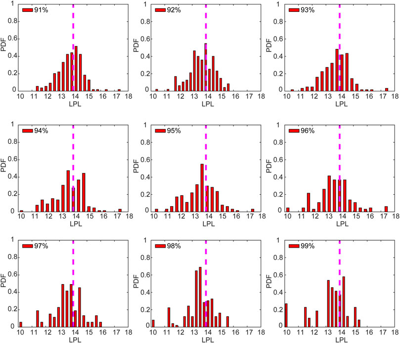
FIGURE 6. Probability histograms of the LPLs of extreme warm events in different percentiles. Pink dashed lines denote LPL = 14 tus.

Figure 7 shows the probability histograms of extreme cold events for different percentiles. The probabilities are at a maximum when the LPLs are 13–14 tus. In general, the LPLs of the extreme cold events also have a Gaussian-like distribution. However, the proportion of the LPLs of extreme cold events at <14 tus is higher than for the extreme warm events. This indicates that the LPLs of extreme cold events have lower values as compared with the extreme warm events.

FIGURE 7

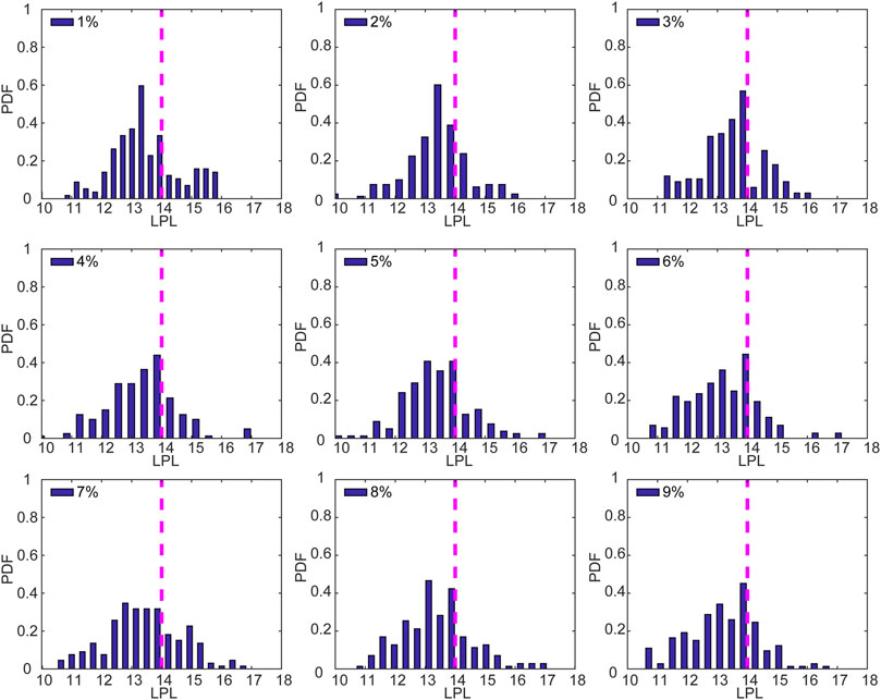
FIGURE 7. Same as for Figure 6, but for extreme cold events.

To verify this, we calculated the cumulative distribution functions (CDFs) of the extreme warm and cold events (Figure 8). Similar to the probability, the LPLs of the extreme warm events are always higher than those of the extreme cold events. Therefore, the LPLs of the extreme warm events have higher values.

FIGURE 8

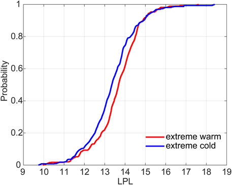
FIGURE 8. CDF curves for extreme warm and cold events.

We also statistically analyzed the LPLs of the two types of extreme events. Figure 9 is a box-and-whisker plot of the LPLs for all the extreme warm and cold events. It shows the minimum, first quartile, median, third quartile, and maximum of the extreme events. The maximum LPL of the extreme warm events is >16 tus, which is higher than that of the extreme cold events (∼16 tus). The other four statistical parameters exhibit similar differences as the maximum (Table 1). Therefore, the LPLs of the extreme warm events are higher than those of the extreme cold events.

FIGURE 9

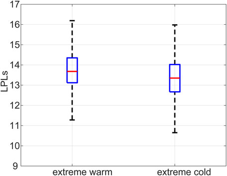
FIGURE 9. Box-and-whisker plot of the LPLs for all the extreme warm and cold events.

TABLE 1

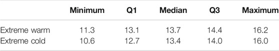
TABLE 1. Statistical parameters for the LPLs of the extreme warm and cold events.

Figure 10 shows the PDFs of the LPLs of the two types of extreme events. When the LPL of the extreme warm events is 13.6 tus, the probability reaches a maximum value (0.35). For the extreme cold events, the maximum probability is 0.33, at LPL = 13.4 tus. When the LPL is <13.2 tus, the probabilities of the extreme cold events are always higher than those of the extreme warm events. For a LPL >13.2 tus, the opposite is the case. Therefore, the LPLs of the extreme warm events are higher than for extreme cold events. Therefore, the CDFs, statistical parameters, and PDFs of the two types of extreme events show that extreme warm events have higher LPLs, and thus are more predictable than extreme cold events.

FIGURE 10

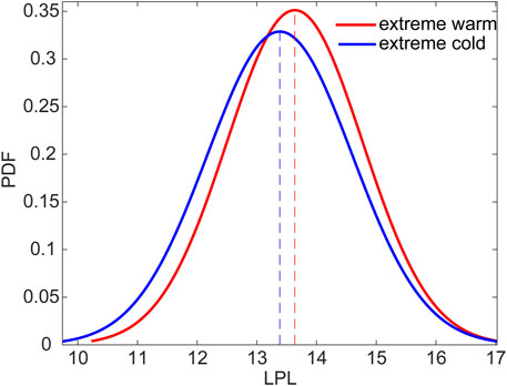
FIGURE 10. PDF curves of the LPLs for the warm and cold events. The red and blue dashed lines denote the LPLs of the extreme warm and cold events where the probabilities are at a maximum.

Discussion and Conclusion

Extreme weather events are having increasingly significant impacts on society due to global warming, in terms of both frequency and magnitude. However, forecasting such extreme events is challenging. In this paper, we have introduced a new method (BNLLE) to investigate the predictability of extreme events. The theoretical model is able to perform large numbers of numerical simulations at a relatively low computational cost. In addition, the theoretical model (i.e., the Lorenz63 model) can mimic the dynamical properties of the atmosphere.

In a dynamical system, large numbers of initial error vectors perturbed on an initial condition will increase with time. At a specific time (i.e., c), the information of the initial condition is lost, along with the predictability. Thus, the predictability limit from the initial condition can be determined. For the BNLLE method, it is important to find the corresponding initial state of the extreme state. If sufficient initial error vectors are perturbed on an initial state $x\left({\text{t}}_{in}\right)$ and increase to reach climatology at the time of the extreme state $x\left({\text{t}}_{ex}\right)$, the initial state $x\left({\text{t}}_{in}\right)$ is the corresponding initial state. The time interval between $x\left({\text{t}}_{in}\right)$ and $x\left({\text{t}}_{ex}\right)$ is the LPL of the extreme event. Compared with the FTLE method used by Sterk et al. (2012), the BNLLE method takes into account the nonlinearity produced by the chaotic nature of the dynamical system. In addition, the magnitude of the initial errors can be a finite quantity. For the FTLE method, the magnitude of the initial errors is assumed to be infinitesimally small, which may not correspond to the situation of the actual atmosphere.

To quantitatively estimate the LPLs of the extreme events, we firstly obtained the extreme warm and cold events in the Lorenz63 model, based on the relative threshold method. The BNLLE method was then used to quantitatively estimate the LPLs of these extreme warm and cold events. The spatial distribution of the LPLs has a layered structure, whereby the LPLs of events on an individual orbit around the center of either regime are broadly the same, whereas the LPLs are not the same for events on different orbits. Li et al. (2020a) noted that the events on an individual orbit around the center of either regime may have similar dynamical properties, which leads to similar LPLs. Different LPLs characterize events on different orbits due to the variable dynamical properties of the different orbits. Our results also show that the LPLs of the extreme warm and cold events have different values in different percentiles (Figures 4, 5). Extreme warm or cold events with similar dynamical properties will have similar LPLs, leading to a smaller standard deviation. This probably enhances the forecast skill for such events. Therefore, the standard deviation can qualitatively reflect the average predictability of events in a group. The spread here represents the standard deviation. A larger spread reflects a lower average LPL for extreme events in a group and vice versa. The range of the LPLs for the two types of extreme events does not decrease or increase gradually as the magnitude of the extreme events increase (Figures 4, 5). This suggests other factors, in addition to the magnitude of the extreme events, affect the predictability. These factors may include the spatial position of the dynamical flow, error magnitudes, and structure of the Lorenz attractor. In addition, we also apply the BNLLE method to quantify the local predictability of an extreme heatwave event in late June 2019, in Europe. This temperature keeps rising from 21 June 2019, and reaches the maximum on 27 June 2019. Using the BNLLE method, the initial forecast errors started from June 17 grow to reach saturation on June 27. Therefore, the predictability limit of the extreme heatwave events is 10 days. The GCMs are important tools to study the atmospheric predictability. The GCM employed by the ECMWF has the best performances. GCMs used by other centers like the NCEP also have high forecast skills. The distributions of LPLs for extreme warm and cold events both have a Gaussian-like distribution. The maximum probabilities occur when the LPLs are 13–14 tus for the two types of events. However, at the same probability, the LPLs of the extreme warm events are always higher than those of the extreme cold events. This indicates that the LPLs of the extreme warm events are higher than for the extreme cold events. The minimum, first quartile, median, third quartile, and maximum of the LPLs for the extreme events also show that the LPLs of the extreme warm events are higher than those of the extreme cold events. Similarly, the PDFs suggest that the LPLs of the extreme warm events are higher than those of the extreme cold events. Therefore, our results demonstrate that extreme warm events are more predictable than extreme cold events. Due to the simplicity of the Lorenz63 model as compared with the actual atmosphere, more sophisticated atmospheric and climate modeling is needed to verify this hypothesis.

Data Availability Statement

The raw data supporting the conclusion of this article will be made available by the authors, without undue reservation.

Author Contributions

XL and RD designed and conducted the research and analysis. XL prepared the initial draft. RD and JL reviewed the initial draft and gave some suggestions.

Funding

This research was jointly supported by the Ministry of Science and Technology of the People’s Republic of China (Grant No. 2020YFA0608802), the National Natural Science Foundation of China (Grants Nos 42005054 and 41975070) and China Postdoctoral Science Foundation (Grant No. 2020M681154).

Conflict of Interest

The authors declare that the research was conducted in the absence of any commercial or financial relationships that could be construed as a potential conflict of interest.

Publisher’s Note

All claims expressed in this article are solely those of the authors and do not necessarily represent those of their affiliated organizations, or those of the publisher, the editors and the reviewers. Any product that may be evaluated in this article, or claim that may be made by its manufacturer, is not guaranteed or endorsed by the publisher.

Acknowledgments

Forecast of surface temperature are from TIGGE data (https://apps.ecmwf.int/datasets/data/tigge/levtype=sfc/type=pf/). TIGGE (The Interactive Grand Global Ensemble) is an initiative of the World Weather Research Programme (WWRP). The ERA-interim analysis is used for the observation data (https://apps.ecmwf.int/datasets/data/interim-full-daily/levtype=sfc/). The numerical experiments in this study were carried out at the High-End Computing Center of Fudan University.

Supplementary Material

The Supplementary Material for this article can be found online at: https://www.frontiersin.org/articles/10.3389/fenvs.2022.825233/full#supplementary-material

References

Bódai, T. (2015). Predictability of Threshold Exceedances in Dynamical Systems. Physica D: Nonlinear Phenomena 313, 37–50. doi:10.1016/j.physd.2015.08.007

CrossRef Full Text | Google Scholar

Bougeault, P., Toth, Z., Bishop, C., Brown, B., Burridge, D., Chen, D. H., et al. (2010). The THORPEX Interactive Grand Global Ensemble. Bull. Amer. Meteorol. Soc. 91, 1059–1072. doi:10.1175/2010BAMS2853.1

CrossRef Full Text | Google Scholar

Campos, R. M., Alves, J.-H. G. M., Penny, S. G., and Krasnopolsky, V. (2020). Global Assessments of the NCEP Ensemble Forecast System Using Altimeter Data. Ocean Dyn. 70 (3), 405–419. doi:10.1007/s10236-019-01329-4

CrossRef Full Text | Google Scholar

Dee, D. P., Uppala, S. M., Simmons, A. J., Berrisford, P., Poli, P., Kobayashi, S., et al. (2011). The ERA-Interim Reanalysis: Confguration and Performance of the Data Assimilation System. Q. J. R. Meteorol. Soc. 137 (656), 553–597. doi:10.1002/qj.828

CrossRef Full Text | Google Scholar

Ding, R., and Li, J. (2007). Nonlinear Finite-Time Lyapunov Exponent and Predictability. Phys. Lett. A 364 (5), 396–400. doi:10.1016/j.physleta.2006.11.094

CrossRef Full Text | Google Scholar

Ding, R. Q., Li, J. P., and Kyung-Ja, H. A. (2008). Nonlinear Local Lyapunov Exponent and Quantification of Local Predictability. Chin. Phys. Lett. 25 (5), 1919–1922. doi:10.1088/0256-307X/25/5/109

CrossRef Full Text | Google Scholar

Dosio, A., Mentaschi, L., Fischer, E. M., and Wyser, K. (2018). Extreme Heat Waves under 1.5 °C and 2 °C Global Warming. Environ. Res. Lett. 13 (5), 054006. doi:10.1088/1748-9326/aab827

CrossRef Full Text | Google Scholar

Duan, W., and Mu, M. (2009). Conditional Nonlinear Optimal Perturbation: Applications to Stability, Sensitivity, and Predictability. Sci. China Ser. D-Earth Sci. 52 (7), 883–906. doi:10.1007/s11430-009-0090-3

CrossRef Full Text | Google Scholar

Evans, E., Bhatti, N., Pann, L., Kinney, J., Peña, M., Yang, S.-C., et al. (2004). RISE: Undergraduates Find that Regime Changes in Lorenz's Model Are Predictable. Bull. Amer. Meteorol. Soc. 85 (4), 520–524. doi:10.1175/bams-85-4-520

CrossRef Full Text | Google Scholar

Franzke, C. (2012). Predictability of Extreme Events in a Nonlinear Stochastic-Dynamical Model. Phys. Rev. E 85 (3), 8. doi:10.1103/PhysRevE.85.031134

PubMed Abstract | CrossRef Full Text | Google Scholar

Göber, M., Wilson, C., Milton, S. F., and Stephenson, D. (2004). Fairplay in the Verification of Operational Quantitative Precipitation Forecasts. J. Hydrol. 288 (1-2), 225–236. doi:10.1016/j.jhydrol.2003.11.016

CrossRef Full Text | Google Scholar

Goodliff, M., Fletcher, S., Kliewer, A., Forsythe, J., and Jones, A. (2020). Detection of Non‐Gaussian Behavior Using Machine Learning Techniques: A Case Study on the Lorenz 63 Model. J. Geophys. Res-Atmos. 125 (2), e2019JD031551. doi:10.1029/2019jd031551

CrossRef Full Text | Google Scholar

Hallerberg, S., and Kantz, H. (2008a). Influence of the Event Magnitude on the Predictability of an Extreme Event. Phys. Rev. E 77 (1), 12. doi:10.1103/PhysRevE.77.011108

PubMed Abstract | CrossRef Full Text | Google Scholar

Hallerberg, S., and Kantz, H. (2008b). How Does the Quality of a Prediction Depend on the Magnitude of the Events under Study? Nonlin. Process. Geophys. 15 (2), 321–331. doi:10.5194/npg-15-321-2008

CrossRef Full Text | Google Scholar

Hallerberg, S., Altmann, E. G., Holstein, D., and Kantz, H. (2007). Precursors of Extreme Increments. Phys. Rev. E 75 (1), 13. doi:10.1103/PhysRevE.75.016706

PubMed Abstract | CrossRef Full Text | Google Scholar

Howe, P. D., Marlon, J. R., Wang, X., and Leiserowitz, A. (2019). Public Perceptions of the Health Risks of Extreme Heat Across US States, Counties, and Neighborhoods. Proc. Natl. Acad. Sci. USA 116 (14), 6743–6748. doi:10.1073/pnas.1813145116

PubMed Abstract | CrossRef Full Text | Google Scholar

Kantz, H., Holstein, D., Ragwitz, M., Vitanov, N. K., and Applications, I. (2004). Markov Chain Model for Turbulent Wind Speed Data. J. Physica A: Stat. Mech. 342 (1-2), 315–321. doi:10.1016/j.physa.2004.01.070

CrossRef Full Text | Google Scholar

Laaidi, K., Zeghnoun, A., Dousset, B., Bretin, P., Vandentorren, S., Giraudet, E., et al. (2012). The Impact of Heat Islands on Mortality in Paris during the August 2003 Heat Wave. Environ. Health Perspect. 120 (2), 254–259. doi:10.1289/ehp.1103532

PubMed Abstract | CrossRef Full Text | Google Scholar

Lamper, D., Howison, S. D., and Johnson, N. F. (2001). Predictability of Large Future Changes in a Competitive Evolving Population. Phys. Rev. Lett. 88 (1), 017902. doi:10.1103/PhysRevLett.88.017902

PubMed Abstract | CrossRef Full Text | Google Scholar

Li, X., Ding, R., and Li, J. (2019). Determination of the Backward Predictability Limit and its Relationship with the Forward Predictability Limit. Adv. Atmos. Sci. 36 (6), 669–677. doi:10.1007/s00376-019-8205-z

CrossRef Full Text | Google Scholar

Li, X., Ding, R., and Li, J. (2020a). Quantitative Comparison of Predictabilities of Warm and Cold Events Using the Backward Nonlinear Local Lyapunov Exponent Method. Adv. Atmos. Sci. 37 (9), 951–958. doi:10.1007/s00376-020-2100-5

CrossRef Full Text | Google Scholar

Li, X., Ding, R., and Li, J. (2020b). Quantitative Study of the Relative Effects of Initial Condition and Model Uncertainties on Local Predictability in a Nonlinear Dynamical System. Chaos. Solitons Fractals 139, 110094. doi:10.1016/j.chaos.2020.110094

CrossRef Full Text | Google Scholar

Li, X., Feng, J., Ding, R., and Li, J. (2021). Application of Backward Nonlinear Local Lyapunov Exponent Method to Assessing the Relative Impacts of Initial Condition and Model Errors on Local Backward Predictability. Adv. Atmos. Sci. 38 (9), 1486–1496. doi:10.1007/s00376-021-0434-2

CrossRef Full Text | Google Scholar

Lorenz, E. N. (1963). Deterministic Nonperiodic Flow. J. Atmos. Sci. 20 (2), 130–141. doi:10.1175/1520-0469(1963)020<0130:dnf>2.0.co;2

CrossRef Full Text | Google Scholar

Matsueda, T. (2008). Can MCGE outperform the ECMWF ensemble? SOLA 4, 77–80. doi:10.2151/sola.2008-020

CrossRef Full Text | Google Scholar

Mu, M., and Duan, W. (2003). A New Approach to Studying ENSO Predictability: Conditional Nonlinear Optimal Perturbation. Chin.Sci.Bull. 48 (10), 1045–1047. doi:10.1007/bf03184224

CrossRef Full Text | Google Scholar

Mu, M., Xu, H., and Duan, W. (2007). A Kind of Initial Errors Related to “spring Predictability Barrier” for El Niño Events in Zebiak‐Cane Model. Geophys. Res. Lett. 34 (3), 27412. doi:10.1029/2006gl027412

CrossRef Full Text | Google Scholar

Nastac, G., Labahn, J. W., Magri, L., and Ihme, M. (2017). Lyapunov Exponent as a Metric for Assessing the Dynamic Content and Predictability of Large-Eddy Simulations. Phys. Rev. Fluids 2 (9), 094606. doi:10.1103/physrevfluids.2.094606

CrossRef Full Text | Google Scholar

Nayak, S., and Takemi, T. (2019). Dynamical Downscaling of Typhoon Lionrock (2016) for Assessing the Resulting Hazards under Global Warming. J. Meteorol. Soc. Jpn. 97 (1), 69–88. doi:10.2151/jmsj.2019-003

CrossRef Full Text | Google Scholar

Nese, J. M. (1989). Quantifying Local Predictability in Phase Space. Physica D 35 (1-2), 237–250. doi:10.1016/0167-2789(89)90105-x

CrossRef Full Text | Google Scholar

Palmer, T. N. (1993). Extended-Range Atmospheric Prediction and the Lorenz Model. Bull. Amer. Meteorol. Soc. 74 (1), 49–65. doi:10.1175/1520-0477(1993)074<0049:erapat>2.0.co;2

CrossRef Full Text | Google Scholar

Sterk, A. E., and van Kekem, D. L. (2017). Predictability of Extreme Waves in the Lorenz-96 Model Near Intermittency and Quasi-Periodicity. Complexity 2017, 9419024. doi:10.1155/2017/9419024

CrossRef Full Text | Google Scholar

Sterk, A. E., Holland, M. P., Rabassa, P., Broer, H. W., and Vitolo, R. (2012). Predictability of Extreme Values in Geophysical Models. Nonlin. Process. Geophys. 19 (5), 529–539. doi:10.5194/npg-19-529-2012

CrossRef Full Text | Google Scholar

Sterk, A. E., Stephenson, D. B., Holland, M. P., and Mylne, K. R. (2016). On the Predictability of Extremes: Does the Butterfly Effect Ever Decrease? Q.J.R. Meteorol. Soc. 142 (694), 58–64. doi:10.1002/qj.2627

CrossRef Full Text | Google Scholar

Sun, Q., Miao, C., Hanel, M., Borthwick, A. G. L., Duan, Q., Ji, D., et al. (2019). Global Heat Stress on Health, Wildfires, and Agricultural Crops under Different Levels of Climate Warming. Environ. Int. 128, 125–136. doi:10.1016/j.envint.2019.04.025

PubMed Abstract | CrossRef Full Text | Google Scholar

Swinbank, R., Kyouda, M., Buchanan, P., Froude, L., Hamill, T. M., Hewson, T. D., et al. (2016). The TIGGE Project and its Achievements. Bull. Amer. Meteorol. Soc. 97, 49–67. doi:10.1175/BAMS-D-13-00191.1

CrossRef Full Text | Google Scholar

Thompson, P. D. (1957). Uncertainty of Initial State as a Factor in the Predictability of Large Scale Atmospheric Flow Patterns. Tellus 9 (3), 275–295. doi:10.3402/tellusa.v9i3.9111

CrossRef Full Text | Google Scholar

Vallejo, J. C., and Sanjuán, M. A. F. (2013). Predictability of Orbits in Coupled Systems through Finite-Time Lyapunov Exponents. New J. Phys. 15 (11), 113064. doi:10.1088/1367-2630/15/11/113064

CrossRef Full Text | Google Scholar

Vannitsem, S. (2017). Predictability of Large-Scale Atmospheric Motions: Lyapunov Exponents and Error Dynamics. Chaos 27 (3), 032101. doi:10.1063/1.4979042

PubMed Abstract | CrossRef Full Text | Google Scholar

Yoden, S., and Nomura, M. (1993). Finite-Time Lyapunov Stability Analysis and its Application to Atmospheric Predictability. J. Atmos. Sci. 50 (11), 1531–1543. doi:10.1175/1520-0469(1993)050<1531:ftlsaa>2.0.co;2

CrossRef Full Text | Google Scholar