 Luciana Staiano
 Federico Gallego
 Alice Altesor3
- 1Laboratorio de Análisis Regional y Teledetección (LART), IFEVA, CONICET, Facultad de Agronomía, Universidad de Buenos Aires, Buenos Aires, Argentina
- 2Departamento de Métodos Cuantitativos y Sistemas de Información, Facultad de Agronomía, Universidad de Buenos Aires, Buenos Aires, Argentina
- 3Instituto de Ecología y Ciencias Ambientales, Facultad de Ciencias, Universidad de la República, Montevideo, Uruguay
- 4Instituto Nacional de Investigación Agropecuaria (INIA), Estación Experimental La Estanzuela, Colonia, Uruguay
Grasslands of southern South America are being replaced by annual crops and forest plantations. The environmental and social consequences of this expansion generate the need for its regulation. If a conservation policy were established, it would be critical to define which areas would have priority for conservation. Multi-criteria analysis techniques are useful tools in territorial planning processes since they allow incorporating diverse and even opposing opinions and objectives. We present a methodological approach to define the Grasslands’ Conservation Value (GCV) from a spatially explicit territorial diagnosis, based on multiple criteria and incorporating explicitly and quantitatively the valuations and opinions of stakeholders. The study was developed as part of the strategy of a public inter-institutional entity to contribute in defining grasslands conservation policies. The methodological approach included workshops in which the definitions of the conservation criteria and their weighting were agreed upon. Definitions were based on a multidimensional technical characterization of the territory through indicators, for which the information used was compiled, analyzed, shared, and synthesized. Based on multi-criteria analysis, each of 12 stakeholders’ groups representatives established the individual weighting of the criteria for determining the GCV and then, established a consensus weighting. The GCV was mapped by integrating territorial diagnosis of these criteria with the weightings carried out by the stakeholders. The degree of agreement among stakeholders in the differential valuation of the ecological criteria was high for 8 of the 12 stakeholders (Pearson’s correlation coefficients >0.92), showing a high agreement between their opinions and those resulting from the group consensus. In all cases, the agreement about the spatial variation of conservation value was higher than on the criteria weights (Pearson’s correlation coefficients ≥0.92 for 10 stakeholders). Furthermore, the sites with lower values in the consensus map corresponded mostly to those sites with lower agreement among stakeholders. The proposed methodology allowed the incorporation of different perceptions not only in the definition of conservation criteria but also in their prioritization, in a transparent and auditable process. This could contribute to the implementation of future regulations that restrict the replacement of grasslands, increasing the legitimacy of territorial planning processes.
1 Introduction
Temperate grasslands are one of the most threatened biomes (Sala, 2001; Carbutt et al., 2017) with one of the highest habitat losses and the smallest protected area at global scale (Hoekstra et al., 2005). During the last decades, land-use changes determined the loss of extensive areas of native grasslands in South America (Paruelo et al., 2006; Baldi and Paruelo, 2008; Hansen et al., 2013; Salazar et al., 2015). This process is part of a global trend where many factors interplay to determine these changes (Geist and Lambin, 2002; Modernel et al., 2016; Volante et al., 2016). Among them, land grabbing processes, commodities prices, and technological changes have been identified as major drivers (Borras et al., 2012; Rulli et al., 2013). In particular, the temperate grasslands of southern South America -Río de la Plata Grasslands region-represent one of the most extensive grassland ecosystems in the Neotropics (Soriano et al., 1992). In this region, the area of native grasslands was reduced by 19.4% between 2000 and 2019 (Mapbiomas Pampa, 2021). In the Uruguayan portion two type of transformations took place. On the one hand, an increase in the area devoted to annual crops (mainly soybean) and, on the other, an expansion of forest plantations (mainly Eucalyptus and Pinus) (Baldi and Paruelo, 2008; Vega et al., 2009; Oyarzabal et al., 2019; FAO, 2020). The environmental and social consequences of this process (Brazeiro et al., 2008; Piñeiro, 2010; Eclesia et al., 2012; Texeira et al., 2015) highlighted the need to regulate agricultural and forestry expansion (Paruelo et al., 2006). In fact, a Law that regulate forest plantations expansion is current under debate in the Uruguayan Congress (Parlamento del Uruguay, 2021).
If a conservation policy for natural grasslands were established, it would be critical to define which areas would have a priority for conservation. The criteria for assigning a high conservation value in an area were, historically, associated with the biodiversity preservation (Margules and Usher, 1981; Daniels et al., 1991; Scott et al., 1993; Humphries et al., 1995; Margules and Pressey, 2000; Egoh et al., 2007), which was the accepted overall objective of conservation policies for decades (Callicott et al., 1999). Recently, a more general concern for maintaining the capacity of ecosystems to sustain and regulate processes (e.g., nutrient and water dynamics, and carbon balance) has gained consensus (Goldman et al., 2008; Naidoo et al., 2008). Such concern is clearly related to the link between ecosystem functioning and the Ecosystem Services (ES) supply (Fisher and Turner, 2009; Haines-Young and Potschin, 2010). Noss (1990) provide an integrative view of the biodiversity concept including not only compositional aspects but also structural and functional dimensions at different levels of organization, from genes to landscapes. Even considering a broader definition of biodiversity and including other ecological criteria it is critical to also consider the human component and its interaction (Collins et al., 2011). In many cases, conservation planning failed due to insufficient consideration of social, economic, cultural, or institutional aspects (Ban et al., 2013). To identify which criteria related to the human dimension are important, why they are important, and how they should be quantified, integrated, and interpreted has proven a challenge (Pacheco-Romero et al., 2020). In this context, the subject of conservation should be the socio-ecosystem (Berkes et al., 2000) and given that the conservation value is linked to the capacity to provide ES (Eastwood et al., 2016), it should be characterized at the level those services are provided, the landscape. At this level occurs the most intense interactions between people and nature, consequently the composition and configuration of a landscape deeply affect and are affected by human activities (Wu, 2013).
Another critical aspect when a conservation policy is planned is who will determine the priority areas for conservation. As both the representativeness of the stakeholders and their ability to influence the results of the process increase, legitimacy in the implementation of these results is likely to increase as well (Reed, 2008; Aguiar et al., 2018). In turn, successful implementation of the results will depend on conservation interventions that are ecologically appropriate and socially acceptable (Ban et al., 2009; Dudley and Stolton, 2010). In this sense, stakeholder’s participation in the prioritization of conservation needs is key to increasing the legitimacy and transparency of decisions. To incorporate the opinions and visions of the different stakeholders is a major challenge, as the process is influenced by the social (Auer et al., 2020) and symbolic (Benn and Jones, 2009) capital of the stakeholders and by the power relationships among them (Reed, 2008; Sterling et al., 2019). Furthermore, given that decisions are based on the interaction between values, interests, emotions (Levine et al., 2015) and available evidence (Sterling et al., 2017), specific methods are needed that consider this complexity of factors (Mukherjee et al., 2018). One way to do this is to explicitly separate the objective and subjective components of this process. For this, is critical to generate mechanisms to make explicit and document both, the criteria that are considered to determine the conservation value and how they are spatially applied, as well as the different perceptions of stakeholders involved in the process.
Multi-criteria analysis techniques are very useful tools in territorial planning processes, since they allow diverse opinions to be considered and the coexistence of opposing objectives or visions (Saaty, 1977, 2014; Saaty and Peniwati, 2008). This method makes it possible to quantify, record and document systematically the different opinions, bringing transparency to the decision-making process. However, many of the studies that use these techniques for conservation-related decision-making do not involve stakeholders in the formulation of criteria and weight them based on hierarchies defined by experts, instead of collecting stakeholder concerns (Esmail and Geneletti, 2018). In turn, often some techniques are used to reduce the variability of stakeholder weightings (Proctor and Drechsler, 2006), which does not allow assessing the degree of agreement among them. The studies linked to the prioritization of conservation areas in Uruguay, were based exclusively on ecological aspects and weighting of criteria was defined by experts (Bilenca and Miñarro, 2004; Soutullo et al., 2013; di Minin et al., 2017; Brazeiro et al., 2020).
In this article we present and apply a novel methodological approach to characterize the Grasslands’ Conservation Value (GCV) from a spatially explicit territorial diagnosis based on multiple criteria (ecological and socioeconomic) and incorporating explicitly and in quantitative terms the assessments and opinions of stakeholders. From the results of the process, we quantify the degree of agreement among stakeholders both in the differential assessment of the criteria and in the spatial variation of the conservation value. We also evaluate which criteria contribute to the differentiation of the assessments. The analyses were performed in the South-Central region of Uruguay, in the Río de la Plata Grasslands, which is undergoing profound land-use and land-cover changes. The process was carried out as part of the strategy of a public inter-institutional entity to contribute to the definition of grassland conservation policies.
2. Methods
2.1 Case description and study area
As part of the concern on the sustainability of cattle production on native grasslands, the Ministry of Livestock, Agriculture and Fisheries of Uruguay set up in 2012 the Board of Livestock on Natural Grasslands (“Mesa de Ganadería sobre Campo Natural”, MGCN for its acronym in Spanish). The MGCN is a public inter-institutional entity whose objectives are aimed at the dynamic conservation of grasslands. It includes different institutions: representatives of the research and development system, rural extension, farmers’ associations, non-governmental organizations, international cooperation institutions, and governmental agencies (Supplementary Table S1) (MGCN, 2021). In a context of growing concern about the transformation of grasslands into croplands and forest plantations, the MGCN initiated in 2017 action aimed to make a spatially explicit territorial diagnosis and to characterize the conservation value of grasslands of the South-Central region of Uruguay (Panario, 1987; Panario et al., 2014). This pilot area was selected by the stakeholders given its vulnerability to grassland losses. It has undergone major changes in land-use and is currently seriously threatened by the installation of a new pulp mill (http://upmpasodelostoros.com) that promotes future forestry production projects.
The South-Central region, with 2.3 million hectares, is characterized by gentle hills with soils originated from granitic bedrock and quaternary sediments (Panario et al., 2014). The climate is humid temperate, the average annual temperature is 17°C and the average annual precipitation varies between 1,100 and 1,200 mm per year (INUMET, 2021). Native grasslands, devoted to livestock production, occupied 42% of the South-Central region, annual crops lands (mainly soybean, corn, and winter crops) 54% and forest plantations the remaining 4% (Baeza et al., 2019) (excluding urban areas and water bodies). Two native grasslands communities are present in this region (Lezama et al., 2019). The first one corresponded to sparsely-vegetated grasslands. This community is characterized by meso-xerophytic species and includes stands with shallow or very shallow soils. It has two variants (sub-communities) in the study area, one of them is characterized by Stenachaeniumcampestre-Andropogon ternatus and the other one by Aira elegantissima-Micropsisspathulata (Lezama et al., 2019). The second plant community corresponds to densely-vegetated grasslands dominated by mesophytic species, encompassing stands with high plant cover values (near 100%) that occupied medium and deep soils. Again, this community present two variants in the region, one characterized by the presence of Chevreuliasarmentosa-Danthonia montevidensis and the other by Lolium multiflorum-Nassellacharruana (Lezama et al., 2019).
2.2 Methodology for determining the conservation value
The methodological approach included: 1) three workshops in April, May, and June 2017 in which the definitions of the conservation criteria and their weighting were agreed upon, and 2) technical work where the information to be used was prepared, analyzed, and synthesized (Figure 1). The workshops were convened by the MGCN as part of its regular meetings. Participants included representatives of the different organizations of the MGCN (each of the stakeholders has a representative on the MGCN, Supplementary Table S1) and the technical team (the authors of this article). Although the three workshops were attended by most of the representatives, there were some who participated in only 1 or 2 of the workshops. In the first workshop the criteria and indicators to be included in the territorial diagnosis were presented and discussed. The weightings of the ecological and socioeconomic criteria were carried out in the second and third workshop, respectively.
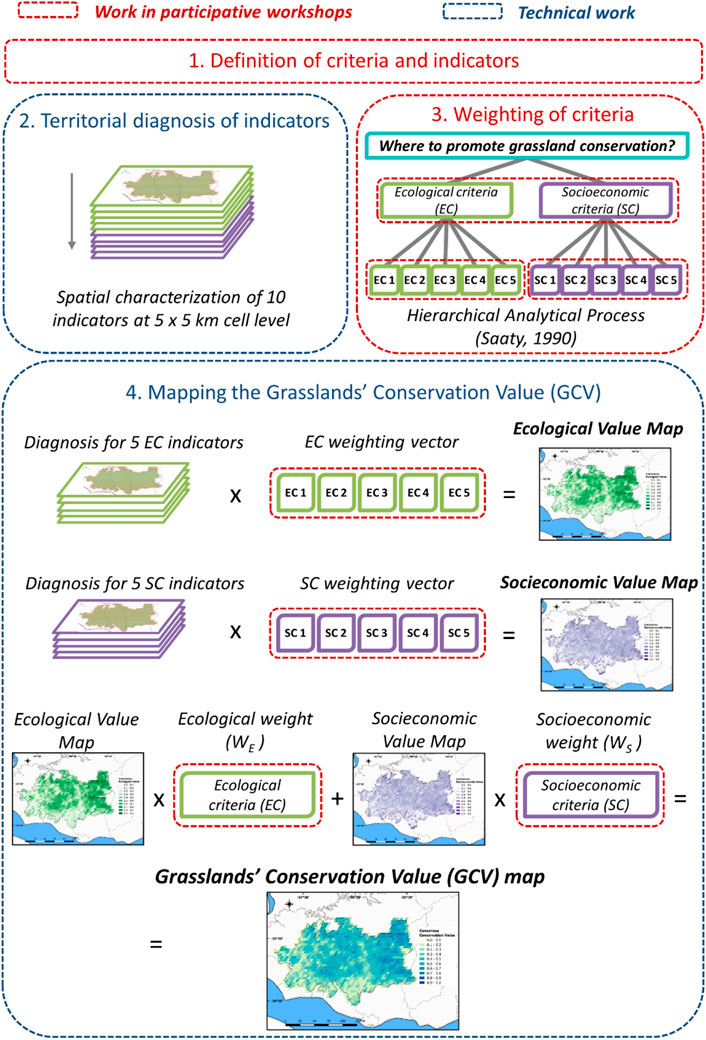
FIGURE 1. Methodological steps for defining the Grasslands’ Conservation Value (GCV). The size of the boxes does not represent the relative importance of each stage in the process.
2.2.1 Criteria and indicators for the socio-ecological diagnosis
The first step included the definition of the criteria on which the conservation value was to be determined (Figure 1). The criteria corresponded to both biophysical and human components of the socio-ecological system. Before the first workshop, the members of the MGCN, in the context of their regular meetings, worked on identifying important criteria to determine the GCV. A first list of criteria resulted from these meetings, and it was provided to the technical team. Indicators for these criteria were derived mainly from two sources, scientific articles and information from public institutions. In the first workshop, based on this proposal, the technical team, based on the previous work of the stakeholders, presented a first proposal of criteria to be included in the socio-ecological diagnosis. Each criterion was characterized by different indicators. Such indicators had to be spatially explicit to geographically discriminate areas with different conservation value. In turn, each indicator was evaluated by the members of the MGCN according to its relevance, source, and scale. Based on the comments of the workshop participants, the criteria and indicators considered were incorporated, modified, or discarded. Some new criteria were incorporated upon the comments of the attendants. A total of 34 indicators corresponding to 15 criteria were mapped and integrated into a Geographic Information System (Quantum GIS software) (Supplementary Table S2). Each indicator was summarized at a spatial resolution of 5 km (Figure 1) and scaled to the range (0–1) to make them comparable, using the following equation:
Where Xi scaled corresponds to the scaled value of indicator X for cell i, Xi is the value taken by indicator X in cell i, Xmin is the minimum value taken by indicator X among all cells and Xmáx is the maximum value taken by indicator X. For each criterion, a single indicator was selected, and correlation analyses were performed between the indicators in each group to rule out redundancies among them (Supplementary Figure S1). In those cases where Pearson correlation coefficient between two indicators was greater than 0.65, only one of them was conserved (e.g., floristic diversity was excluded because it presented a high correlation with the proportion of grasslands, r = 0.98).
As a result, a final set of 10 criteria was agreed in the second workshop (Figure 1). The criteria were divided into two groups (ecological and socioeconomic). In the first group, 5 Ecological Criteria (EC) were included, characterized through 5 indicators (Figure 2, Supplementary Table S3, Supplementary Figure S2):
• EC1: Protected areas and priority sites for conservation, characterized by the presence/absence of both a protected area and areas integrated into the network of priority sites to be incorporated according to a plan proposed by the National System of Protected Areas (SNAP, 2015).
• EC2: Faunal diversity, characterized through 5 maps of potential species richness for mammals, birds, reptiles, amphibians, and fishes in ∼66,000 ha cells for all of Uruguay (Brazeiro et al., 2008). A potential faunal diversity index was determined as the sum of the 5 specific richnesses summarized at the 5 × 5 km cell level.
• EC3: Functional diversity, characterized through the Ecosystem Functional Types (EFT) diversity. The EFT (Paruelo et al., 2001) result from combining three attributes of the annual dynamics of remotely sensed vegetation indices: the annual mean, the intra-annual coefficient of variation, and the moment of year of peak productivity. This approach allows to infer the degree of productive diversity. From the annual dynamics of the Enhanced Vegetation Index (EVI, derived from MODIS sensor images, product Mod13q1 with a spatial resolution of 250 m and a temporal resolution of 16 days), the EFTs were obtained for the year 2015. Four fixed levels were generated for the three attributes that were then combined to generate a map of EFTs (Alcaraz-Segura et al., 2013). The 250-m pixels corresponding to grasslands (identified from the EC4 land cover map corresponding to the same year) were excluded, and the Shannon Index was calculated to describe the functional diversity of the grassland surroundings.
• EC4: Remaining grassland area (proportion), obtained from a land-cover map for 2015, with a spatial resolution 30 m (Baeza et al., 2019).
• EC5: Grasslands’ ecosystem services supply, determined by trends in the Ecosystem Services Supply Index (ESSI), a synoptic indicator that estimates and maps supporting and regulating ecosystem services related to water and carbon dynamics derived from remote sensing data (Paruelo et al., 2016). The support for using ESSI as a proxy of ecosystem service supply is based on its ability to explain between 48 and 66% of the variability of four ecosystem services estimated from empirical data or mechanistic models: groundwater recharge and avian richness in Dry Chaco forests and soil organic carbon and evapotranspiration in Río de la Plata Grasslands (Paruelo et al., 2016). It is based on two attributes of vegetation index annual dynamics, the annual mean (VIMEAN, a proxy of total C gains) and the intra-annual coefficient of variation (VICV, an indicator of seasonality): ESSI = VIMEAN * (1—VICV). Those sites where annual productivity is higher and more seasonally stable would have a higher ES supply. From the annual dynamics of EVI (derived from MODIS sensor images, product Mod13q1 with a spatial resolution of 250 m and a temporal resolution of 16 days), the annual ESSI values were obtained, and their trend was estimated during the period 2000–2015. Since the criterion aimed to capture the ecosystem services supply provided by grasslands in a cell, the proportion of pixels corresponding to grasslands (identified from the EC 4 mapping) without negative ESSI trends (i.e., where the ecosystem services supply has been maintained or increased) was calculated with respect to the total number of grassland pixels in the cell.
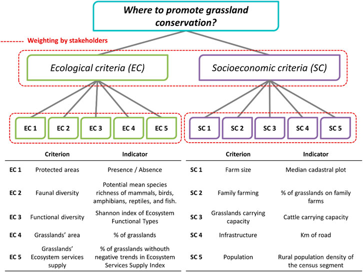
FIGURE 2. Hierarchical structure used to determine the Grasslands’ Conservation Value (GCV). The question to be answered is which cells (5 x 5 km) have higher conservation value. The criteria to answer that question were grouped into two categories: ecological (EC 1 to EC 5) and socioeconomic (SC1 to SC5), which were characterized by a spatially explicit diagnosis of their indicators. Each dotted red box encloses the elements that the stakeholders compared in the three weightings carried out. Each comparison gives rise to a weighting vector representing the relative importance of each element with respect to the others, whose sum is equal to 1.
In the second group, 5 Socioeconomic Criteria (SC) were included, characterized through 5 indicators (Figure 2, Supplementary Table S4, Supplementary Figure S3):
• SC1: Farm size, characterized through the median of cadastral plots (Dirección Nacional de Catastro, 2017).
• SC2: Family farming, whose indicator was the proportion of grasslands in family farms with respect to the total area of grasslands in the cell. One of the stakeholders (representative of The Rural Development office of the Ministry of Livestock, Agriculture and Fisheries) provided the information of the family farms, protecting the identity of the owners.
• SC3: The grasslands carrying capacity was estimated as follows:
• SC4: An index of infrastructure of each cell was characterized through the sum of the kilometers of road of the official national road network (Ministerio de Transporte y Obras Públicas, 2017).
• SC5: Population, characterized by the rural population density reported in the National Census of Population, Housing and Households (Instituto Nacional de Estadísticas, 2011). The most detailed spatial resolution available corresponds to the census segment.
For the EC, stakeholders agreed that the relationship between the values of each indicator and the contribution to conservation value was positive (i.e., higher values of each indicator contribute to a higher conservation value). In the case of the SC, although the stakeholders agreed that these were important criteria to include, they had different opinions regarding the relationship between the values of each indicator and their contribution to the GCV. These discrepancies required prior agreement, as opinions on weighting depends on the direction in which each indicator contributes to the GCV. For 4 of the 5 criteria, the relationship was positive, while for SC1, it was negative: those cells with smaller median size of cadastral plots would have a higher GCV than those with larger median size. Therefore, this indicator was incorporated into the GCV estimation as its complement (1- SC1 scaled). More details on the criteria and indicators considered is presented as supplementary material (details of the indicators calculated for the ecological and socioeconomic criteria are shown in Supplementary Table S3 and Supplementary Table S4, respectively, while the indicators maps are shown in Supplementary Figure S2 and Supplementary Figure S3).
2.2.2 Weighting of criteria
The weighting of the criteria was based on a multi-criteria analysis method, the Analytic Hierarchy Process (Saaty, 1990, 2014). To establish the relative importance of each criterion, the participants make pairwise comparisons of each criterion with respect to the rest using the Saaty scale (Saaty, 1977). The assignment of preferences was established by comparing the importance of the criterion in each row with respect to the criterion in each column in a square matrix (Table 1) through the scale whose values range from 1 to 9 and establish the following priorities:
1 = Equally important
3 = Moderately more important (and conversely 1/3 is moderately less important)
5 = Strongly important (1/5 strongly less important)
7 = Very strongly important (1/7 very strongly less important)
9 = Extremely more important (1/9 extremely less important)
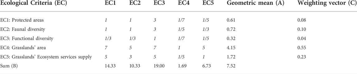
TABLE 1. Example of pairwise criteria comparison and obtaining the weighting vector corresponding to the ecological criteria. The row and column headings contain the criteria compared by the stakeholders using the Saaty scale in italic cells. Once the preferences had been assigned, the geometric mean was calculated for each row of the matrix and the geometric means of all the rows were summarized. The weighting value (relative importance) of each criterion was obtained by dividing its geometric mean (A) by the sum of the geometric means of all rows (7.52). These values determine the weighting vector (C), which indicates the relative importance of each criterion. The last row (B) is used to calculate the consistency level of the matrix.
2, 4, 6, 8 correspond to intermediate values that can be used to resolve compromise situations.
The method provides a measure of the degree of weighting consistency called Consistency Ratio (CR), which indicates to what extent the preferences were assigned through an informed and coherent judgment (Saaty, 1990, 2014). To this, the comparison matrix must comply with 3 properties: reciprocity (e.g., if criterion A is moderately more important than B, then B must be moderately less important than A), transitivity (e.g., if criterion A is more important than B and B is more important than C, then A must be more important than C), and proportionality (e.g., if A is moderately more important than B and B is moderately more important than C, then A must be extremely more important than C). A matrix with CR ≤ 0.10 implies accepting up to 10% of the inconsistency that would have been obtained by chance. If the ratio is much higher than 0.1, the judgments are unreliable because they are too close to randomness (Saaty, 1990, 2014) (see supplementary material for details on consistency analysis).
Based on the hierarchical scheme proposed, the stakeholders made three comparisons (Figure 2). The first one took place during the second workshop, after we presented the results of the ecological indicators diagnosis. Each of the 12 participants compared the 5 ecological criteria with each other using the Saaty scale. Based on the individual preferences a consensus matrix comparison was agreed in a plenary session. This allowed us to calculate an individual weighting vector (anonymous) that summarizes the relative importance that each stakeholder assigned to the ecological criteria and a consensus weighting vector. We also calculated the consistency of each weighting. The second comparison was carried out in the third workshop, after we presented the results of the socioeconomic indicators diagnosis. Each of the participants compared the 5 socioeconomic criteria with each other using the Saaty scale. In this instance, due to the stakeholders’ own dynamics during the workshop, we did not have the individual weightings, but they only registered the consensus weighting of the socioeconomic indicators as agreed in the plenary session. Finally, the relative importance of the ecological criteria with respect to the socioeconomic criteria was determined in plenary session and by consensus. Because at this hierarchical level there is only one pair of elements to compare, we asked them to directly assign a relative importance value. They had to distribute the 100% of the relative importance between the ecological and socio-economic criteria, ecological weighting (WE) and socio-economic weighting (WS), respectively.
2.2.3 Conservation value estimation and mapping
The area was divided into 1,217 cells of 5 × 5 km (Figure 3). Each of these cells represents the entity to which a conservation value will be assigned. The size of the cell was defined based on two criteria: 1) at this resolution (2,500 ha) basic attributes of the landscape (represented elements, configuration and structure) can be characterized (Baldi et al., 2006; Baldi and Paruelo, 2008), and 2) such grain is in between the resolution of coarser (e.g., faunal diversity, human population) and finer (e.g. remaining patches of grassland, supporting and regulating ecosystem services supply) available information. As some of the criteria (e.g., supporting and regulating ecosystem services supply, grasslands carrying capacity, functional diversity) were quantified from such spectral data derived from the MODIS (Moderate Resolution Imaging Spectroradiometer) sensor on board the Terra satellite (Earth Observation System - NASA), the cells of the grid were adjusted to the pixels of the satellite images.
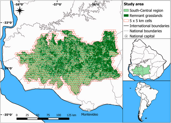
FIGURE 3. Study area. The conservation value has been determined for each cell of 5 x 5 km.
The GCV was determined by integrating the territorial diagnosis of ecological and socioeconomic indicators at the landscape level (5 × 5 km cells), with the weightings carried out by the stakeholders. To incorporate the diagnostic value of the indicators, stakeholders agreed on how each would contribute to conservation value. For 9 of the 10 indicators, a higher diagnostic value corresponded to a higher conservation value (e.g., Faunal diversity, presence of protected areas, carrying capacity, etc.). On the other hand, for the field size criterion, they agreed that higher median area of cadastral parcels would result in a lower conservation value. This was contemplated by performing an inverse scaling for this indicator (Equation 1). First, we determined: 1) the Ecological Value (EV) in each cell (Equation 2), which integrates the diagnostic value of the ecological indicators with the weighting of the ecological criteria by the stakeholders (12 individual weighting vectors and 1 consensus weighting vector) and 2) the Socioeconomic Value (SV) in each cell (Equation 3), which integrates the diagnostic value of the socioeconomic indicators with the weighting carried out in the group consensus. Finally, both values (EV and SV) were integrated together with their weighting (agreed upon in plenary) to obtain the Grasslands’ Conservation Value (GCV) (Equation 4). The three values corresponding to group consensus (EV, SV, and GCV) and the 12 individual EV were mapped.
The EV of each cell (n = 1,217) was determined through the following equation:
Where, EVi corresponds to the Ecological Value of the cell i, j represents the ecological criteria,
The SV of each cell (n = 1,217) was determined through the following equation:
Where, SV corresponds to the Socioeconomic Value of the cell i, k represents the ecological criteria, SC represents the scaled diagnostic value of the indicator describing socioeconomic criterion k for cell i obtained in the territorial diagnosis and
Finally, the conservation value was determined by the weighted sum of EV and SV by their weights (higher hierarchical level) through the following equation:
Where,
2.3 Data analysis and synthesis
The degree of agreement among stakeholders was assessed through two complementary analyses. First, the degree of agreement in both the assessment of the criteria and the mappings was evaluated through correlation analysis (Pearson correlation coefficient, Sokal and Rohlf, 2009), and both analyses were compared to assess the extent to which dissent in the weightings translated into dissent in the maps. Second, from the 12 EV mappings, the Coefficient of Variation (EVCV) was calculated in each of the cells and a map of the degree of agreement in the EV as a complement of the EVCV (1—EVCV) was obtained to identify spatially explicit consensus and disagreement.
3 Results
3.1 Ecological value weightings and mapping
The ecological criteria most highly valued according to the group consensus weighting vector were, in decreasing order of importance, the proportion of grasslands (WEC4 = 0.55) and the level of supply of supporting and regulating ecosystem services (WEC5 = 0.23), followed by faunal biodiversity (WEC2 = 0.10), protected areas (WEC1 = 0.08) and finally functional diversity (WEC3 = 0.04) (Figure 4). The criteria comparison matrix, from which this weighting vector was derived, was consistent (CR = 0.10). As for the individual weights the most highly valued criteria were also the proportion of grasslands and the level of ecosystem services provided by the grasslands and were, in turn, those with the most variable weights among participants (WEC4: mean = 0.44 and SD = 0.19; WEC5: mean 0.26 and SD = 0.12) (Figure 4). Of the 12 individual comparison matrices, 6 were consistent (CR≤0.10 for participants 2, 5, 7, 9, 10, and 12); while of the remaining 6, 3 presented values close to the suggested threshold (CR = 0.17 for participant 1, CR = 0.11 for participant 6 and CR = 0.12 for participant 11) and the other 3 presented higher values (CR = 0.26 for participant 3, CR = 0.27 for participant 4 and CR = 0.41 for participant 8). The individual weighting vectors and their CR are reported in the supplementary material (Supplementary Table S5).
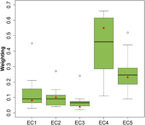
FIGURE 4. Distribution of the weighting values of the 12 individual stakeholders for each of the ecological criteria (EC1: Protected areas, EC2: Faunal diversity, EC 3: Functional diversity, EC4: Remaining grassland area, and EC5: Supporting and regulating ecosystem services supply). In each box, the horizontal black line represents the median, the extremes the quartiles (q1 and q3), the whiskers correspond to 1.5 of the interquartile range and the empty points are outliers. The red triangles represent the weights of the consensus vector.
A total of 73% of the correlations between the individual priority vectors were positive, of which 75% presented correlation coefficients greater than 0.58 and 50% greater than 0.9 (Figure 5). In contrast, 27% of the comparisons presented negative correlation coefficients, of which 50% presented values lower than −0.58 (Figure 5). Higher positive correlation coefficients indicate that the criteria weighting ranking between two stakeholders is similar. More negative coefficients indicate opposite weighting rankings between two stakeholders, while those close to 0 represent different rankings. In this sense, stakeholders P6 and P8 presented negative correlation values with the majority of stakeholders, indicating the lowest degree of agreement (Figure 5). The degree of correlation between each priority vector and the consensus vector was greater than 0.92 for 8 of the 12 stakeholders, showing a high degree of similarity between their rankings and the one resulting from the group consensus (Figure 5). Two of the remaining stakeholders presented positive but lower values (P5 = 0.64 and P7 = 0.44) and the other two negative values (P6 = -0.19 and P8 = -0.63).
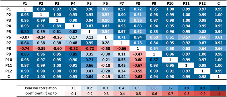
FIGURE 5. Below the diagonal: correlations between the weighting vectors resulting from comparing the ecological criteria among the 12 participants (P1 to P12) and the group consensus (C); values correspond to Pearson’s correlation coefficient (white values indicate significant correlations, p value < 0.05). Above the diagonal: correlations between the Ecological Value (EV) maps of the 12 participants (P1 to P12) and the group consensus (C); values correspond to Pearson's correlation coefficient (white values indicate significant correlations, p value< 0.001).
Regarding the degree of spatial agreement, the correlations between the 12 individual maps and the consensus map was higher or equal than 0.92 for 10 of the 12 stakeholders and for the remaining two it presented values of 0.61 (P6) and 0.66 (P8) (Figure 5). In all cases, the degree of agreement in the maps was higher than in the individual weigthings of criteria, even for the two stakeholders with a low degree of agreement in the individual weigthings of criteria. The dissent of these stakeholders in the weighting of criteria was not reflected in a dissent in the spatial ecological value. In turn, the cells with the lowest EV in the consensus map (Figure 6A), mostly coincide with those cells with the lowest degree of agreement in EV (Figure 6B).
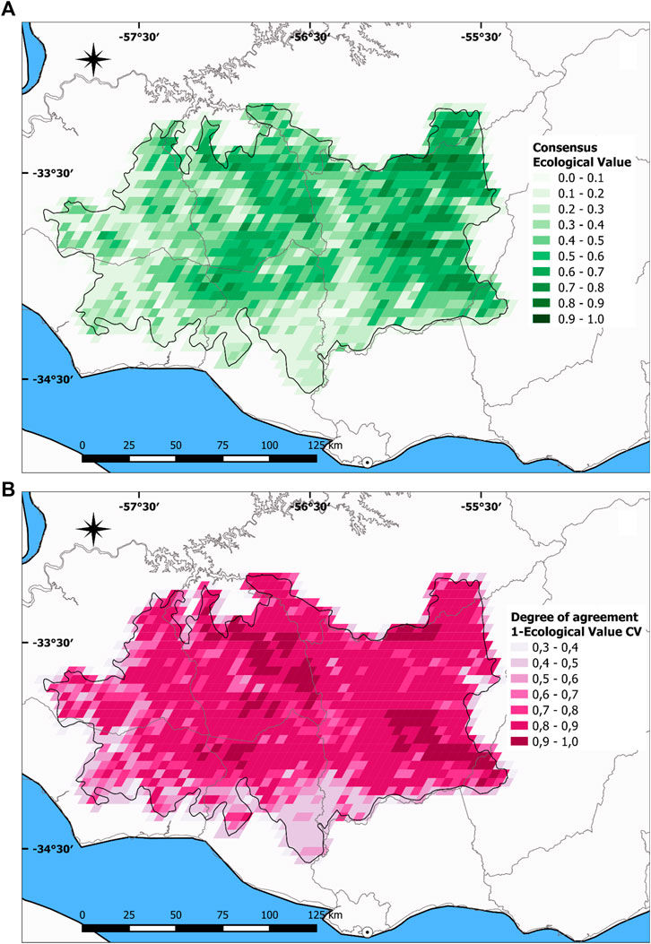
FIGURE 6. Consensus Ecological Value (EV) map (A). Complement of the coefficient of variation of the 12 individual Ecological Value (EV) maps (B).
3.2 Socioeconomic value weighting and grasslands conservation value mapping
The socioeconomic criteria most highly valued according to the group consensus weighting vector were, in decreasing order of importance, grasslands carrying capacity (WSC3 = 0.51) and grasslands on family farms (WSC2 = 0.25), followed by population (WEC5 = 0.12), farm size (WEC1 = 0.08) and finally infrastructure (WEC4 = 0.04). The criteria comparison matrix from which this weighting vector was derived was consistent (CR = 0.03). These results combined with the diagnosis of socioeconomic criteria determined the consensus mapping of socioeconomic value (SV, Figure 7B). The weighting of ecological criteria (WE) to socioeconomic criteria (WS), as determined by group consensus (top level of the hierarchical scheme, Figure 2), was 0.7 and 0.3, respectively. The consensus EV and SV maps weighted by these values determined the GCV map (Figure 7). The consensus EV ranged from 0.07 to 0.84 and the most frequent values were low (21.7% of the area had values between 0.1 and 0.2) (Figures 7A,D). The consensus SV varied between 0.002 and 0.65 and was more homogeneous than the EV, with 73% of the values between 0.3 and 0.5 (Figures 7B,E). The consensus GCV varied between 0.06 and 0.71 and the spatial pattern was similar to that of the EV, but with a higher frequency of average values, since 24.8% of the area had conservation values between 0.4 and 0.5 (Figures 7C,F).
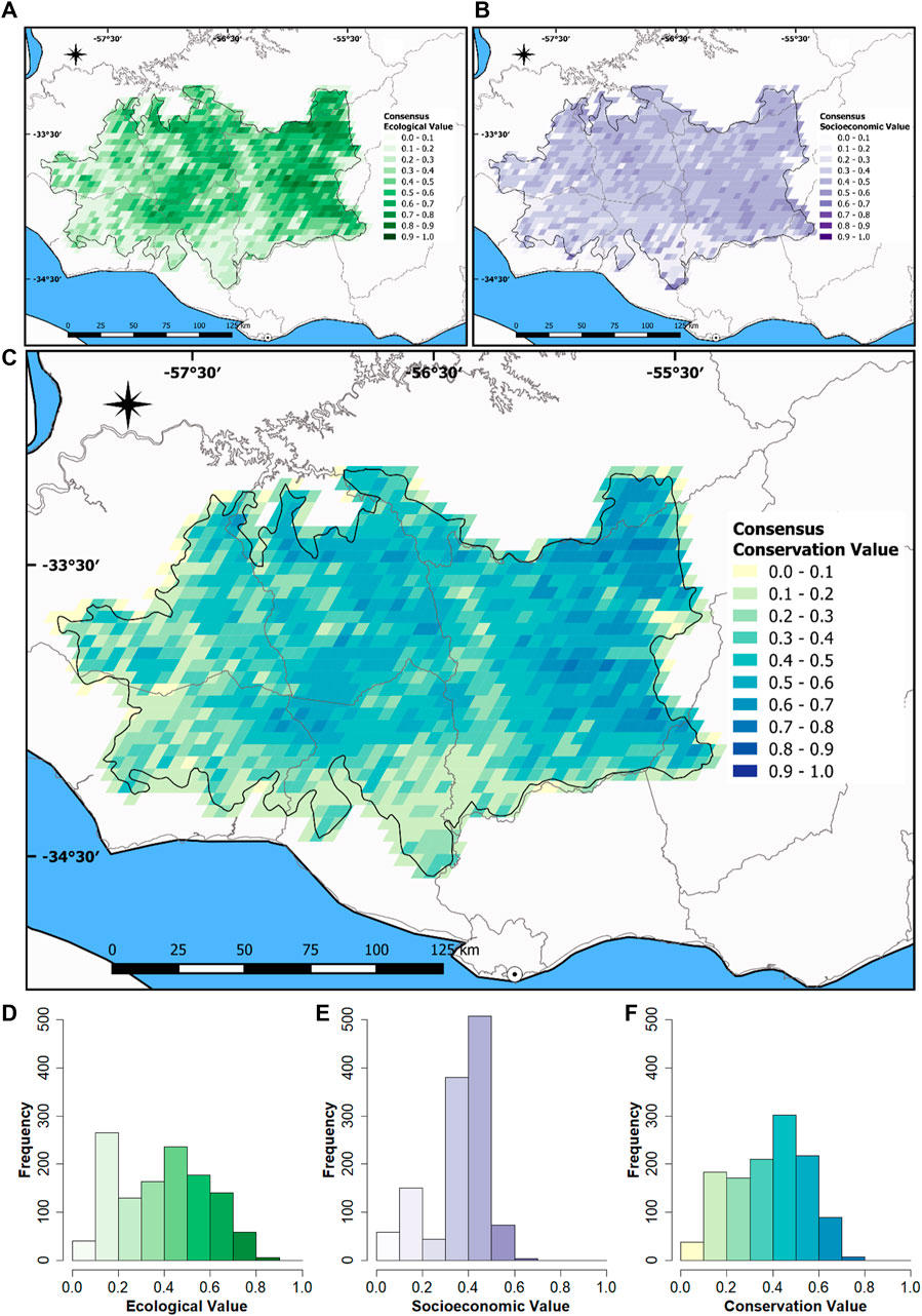
FIGURE 7. Consensus maps and histograms of Ecological Value (EV) (A and D), Socio-economic Value (SV) (B and E) and Grasslands’ Conservation Value (GCV) (C and F).
4 Discussion
Participatory evaluation and decision-making processes face the challenge of incorporating all opinions considering the power relations established among stakeholders (Felipe-Lucia et al., 2015). In this article we presented the development and implementation of a method to quantify the conservation value of natural grasslands based on objective criteria and incorporating the participation of the stakeholders involved. The methodology allowed the incorporation of different perceptions not only in the definition of conservation criteria but also in their prioritization, in a transparent and auditable process. It also made it possible to evaluate the degree of agreement among participants both in the prioritization of criteria and in the grasslands’ conservation value spatial variation.
An a priori and inclusive definition of the criteria to be considered and a critical evaluation of the quality of the data was essential to accommodate all views and interests. The inclusion or exclusion of a criterion in the construction of the conservation value was based on the one hand, on the perception and justification of its importance by the technical team and, at least, one of the stakeholders. On the other hand, the quality of the data was particularly considered. In this sense, spatially explicit data, based on documented sources and with access to metadata were privileged. The scale (extension and resolution) of the information was a key aspect in selecting the data. In this sense, only information that was larger than the area of study was included. Although we tried to include data with a more detailed resolution than that of the defined cells (2,500 ha) to carry out aggregation processes, this was not always possible. In the case of two criteria considered particularly important by some stakeholders (faunal diversity and population density) the basic information was at a coarser resolution. In these cases, we had to downscale the grain of the original information layers. To each cell we assigned the value of the object containing it or an area-weighted average in those cases where the cell overlapped with more than one unit. The lack of spatially explicit information or the availability of information with limited spatial detail highlights the need for the science and technology system to generate more detailed information for the criteria that are important to stakeholders.
The criteria selected to represent the biophysical dimension of the socio-ecosystems sought to cover, at the landscape level, the three dimensions of biodiversity proposed by (Noss, 1990). Thus, aspects related to composition (EC2: potential species richness), structure (EC4: proportion of remaining grassland area) and functioning (EC3: diversity of ecosystem functional types) were included. Along with the biophysical aspects, two aspects related to the interaction between the biophysical and human dimensions were considered (Pacheco-Romero et al., 2020): the presence of protected areas and the change in the supply of regulating and support Ecosystem Services. The criteria associated with the human dimension partially captures the aspects pointed out by Pacheco-Romero et al. (2020). The influence of these criteria in defining conservation value was more controversial than in the case of biophysical aspects. In fact, for some of the criteria the participants disagreed not only on the weight but also on the direction of the influence (positive or negative) on the contribution to the conservation value of grasslands. These disagreements in the direction of influence of the indicators promote major changes in weighting. For example, if a certain stakeholder considered that infrastructure (SC4) was a particularly important criterion and in turn that those areas with a lower degree of infrastructure (SC4) should be those with a higher conservation value, when an inverse (positive) direction was agreed upon for this indicator, the weighting assigned to it was naturally reduced.
Although in study case presented, consensus weights were achieved in the absence of conflict, we consider that there are risks associated with reducing the opinions of multiple stakeholders in a single weighting. There is no consensus in the literature on how to reduce variability in the weights; and the commonly used reductions (some measure of central tendency such as average, median or mode), imply not only that information is lost but also that stakeholders whose weights are very different from the agreed weighting may no longer wish to participate in the process (Proctor and Drechsler, 2006). In this sense, we consider that the most valuable aspect of the method we presented is the possibility of assessing the degree of agreement among stakeholders both in the perception of the criteria (Figure 4, Figure 5) and in the spatial variation of the conservation value (in this case, the ecological value, Figure 6B). Moreover, these aspects were documented and are available to be consulted and discussed in an iterative process. Due to the particular characteristics and dynamics of the MGCN, we did not have the individual priority vectors for the socioeconomic criteria and therefore have not been able to generate individual maps of socioeconomic value (or conservation value), which would be very important to be able to document the degree of agreement on socioeconomic value and its impact on the final GCV. Where and why to conserve grasslands in South-Central region of Uruguay, was associated, according to the stakeholders of the MGCN, mainly, to two criteria. The GCV map resembles the distribution of remnant grasslands (Figure 3, Figure 7C). This is because among the ecological criteria, the area occupied by remanent grasslands was the most important according to group consensus (WEC4 = 0.55, Figure 4). The second most weighted criterion by consensus was Grasslands’ supporting and regulating ecosystem services supply (WEC5 = 0.23, Figure 4), which takes positive values where there were grasslands and zero where there were no grasslands. At the same time, the weighting of the ecological criteria was higher than that of the socioeconomic criteria (WE = 0.7). This implies that those landscapes with few remnant grasslands would not have conservation priority. In this sense, stakeholders raised the possibility of replicating the methodology to answer a different question, which are the areas with the highest restoration priority? In such case a lower proportion of native grasslands and its connectivity would have a greater importance.
Though the stakeholders involved in the processes included the academia, conservation NGOs and ranchers’ associations, the focus was on conservation issues. In temperate and sub-humid grasslands, the exclusion of grazing does not necessarily lead to grassland conservation (Lunt et al., 2007; Cingolani et al., 2008; Gallego et al., 2020). In similar ecosystems, there is evidence that grazing prevents the accumulation of standing dead biomass, increasing light availability and consequently species richness and productivity (Rodríguez et al., 2003; Altesor et al., 2005; Overbeck et al., 2007). In turn, these compositional benefits are reflected in an increase in the supply of supporting and regulating ecosystem services (Gallego et al., 2020). Therefore, grasslands play a key role in supplying both provisioning (meat, wool, water supply) and regulating services (pollination, C sequestration, hydrologic regulation) (Yahdjian et al., 2015). In this sense, the participants weighted the criteria considering that a higher conservation value would imply a restriction for the transformation of grasslands to other land uses, but it would be compatible with cattle production. Thus, a high conservation value would not necessarily imply carrying out strict conservation activities. It is important to note that those stakeholders linked to activities that imply the replacement of grasslands (forestry industries, agricultural companies, for example) were not represented in the MGCN.
The degree of agreement on the prioritization of conservation areas was greater than on the prioritization of criteria, even for participants with a low degree of agreement on the prioritization of criteria. This highlights an important emerging property of the process: the need to postpone the dispute of visions on particular criteria until the results are seen. Some stakeholders differed sharply in the weighting of the presence of protected areas in defining the conservation value. However, given the scarce presence of protected areas in the territory, marked differences in weighting had a low effect on the resulting conservation values. This underscores the importance of postponing discussions and consensus-building until a clear idea of the practical consequences (in this case the GCV assigned) is obtained. The effort to avoid conflicting positions on the importance of each of the criteria should be concentrated on those that have the greatest impact on the final result.
The territorial diagnosis process carried out set the basis to explore the consequences of different scenarios of conservation, transformation, and/or restoration of grasslands areas on critical dimension of the environmental footprint of human activities. Different scenarios of land-use and land-cover can be evaluated in terms of Ecosystem Services supply, natural habitat preservation, functional diversity, and economic output. Aside from its applications, the process was important in itself because it allows the stakeholders to have a clear idea of the dimensions involved in a zoning exercise and to identify gaps in data and conceptual models. Moreover, the methodology implemented not only make visible the range of visions on grassland conservation but also set a productive arena where to discuss alternatives. This could contribute to enrich the decision-making process in the implementation of future regulations restricting grasslands substitution, increasing the legitimacy of territorial planning processes.
Data availability statement
The original contributions presented in the study are included in the article/Supplementary Material, further inquiries can be directed to the corresponding author.
Ethics statement
Ethical review and approval was not required for the study on human participants in accordance with the local legislation and institutional requirements. Written informed consent for participation was not required for this study in accordance with the national legislation and the institutional requirements.
Author contributions
JP, LS, and AA contributed to conception and design of the study. LS and FG organized the database. JP, LS, AA, and FG carried out the field work (participative workshops). LS performed the statistical analysis and wrote the first draft of the manuscript. All authors contributed to manuscript revision, read, and approved the submitted version.
Funding
This article was funded on an agreement between IICA and LART-FAUBA. This research was also financed by Universidad de Buenos Aires (Argentina), Fondo para la Investigación Científica y Tecnológica PICT 2150 (Argentina), Universidad de la República (Uruguay), Programa CSIC Grupos ID 71 (Uruguay), and on a grant from the Inter-American Institute for Global Change Research (IAI) CRN III 3095, which is supported by the US National Science Foundation (Grant GEO-1128040).
Acknowledgments
We thank the members of the MGCN for their participation and willingness to collaborate. Particularly we thank the support and commitment of Marcelo Pereira and Diego Cáceres, President and Secretary of the Board. Sebastián Aguiar, Pablo Baldassini, Gonzalo Camba Sans, Hernán Dieguez, and Paula Torre Zaffaroni contributed to enrich the early discussion of the structure that guided this manuscript. Also, we are grateful to the three reviewers for their comments, which helped us to substantially improve the manuscript.
Conflict of interest
The authors declare that the research was conducted in the absence of any commercial or financial relationships that could be construed as a potential conflict of interest.
Publisher’s note
All claims expressed in this article are solely those of the authors and do not necessarily represent those of their affiliated organizations, or those of the publisher, the editors and the reviewers. Any product that may be evaluated in this article, or claim that may be made by its manufacturer, is not guaranteed or endorsed by the publisher.
Supplementary material
The Supplementary Material for this article can be found online at: https://www.frontiersin.org/articles/10.3389/fenvs.2022.820449/full#supplementary-material
References
Aguiar, S., Mastrangelo, M. E., García Collazo, M. A., Camba Sans, G. H., Mosso, C. E., Ciuffoli, L., et al. (2018). What is the status of the forest law in the chaco region ten years after its enaction? Reviewing its past to discuss its future. Ecol. Austral 28, 400–417. doi:10.25260/ea.18.28.2.0.677
Alcaraz-Segura, D., Paruelo, J. M., Epstein, H. E., and Cabello, J. (2013). Environmental and human controls of ecosystem functional diversity in temperate South America. Remote Sensing 5 (1), 127–154.
Altesor, A., Oesterheld, M., Leoni, E., Lezama, F., and Rodrıguez, C. (2005). Effect of grazing on community structure and productivity of a Uruguayan grassland. Plant Ecol. 179, 83–91. doi:10.1007/s11258-004-5800-5
Auer, A., von Below, J., Nahuelhual, L., Mastrangelo, M., Gonzalez, A., Gluch, M., et al. (2020). The role of social capital and collective actions in natural capital conservation and management. Environ. Sci. Policy 107, 168–178. doi:10.1016/J.ENVSCI.2020.02.024
Baeza, S., Rama, G., and Lezama, F. (2019). “Cartografía de los pastizales naturales en las regiones geomorfológicas de Uruguay predominantemente ganaderas. Ampliación y actualización,” in Bases ecológicas y tecnológicas para el manejo de pastizales II. Editors A. Altesor, L. López-Mársico, J. M. Paruelo, Montevideo, and Serie (Montevideo: FPTA, INIA), 2727–4747.
Baldi, G., Guerschman, J. P., and Paruelo, J. M. (2006). Characterizing fragmentation in temperate South America grasslands. Agric. Ecosyst. Environ. 116, 197–208. doi:10.1016/J.AGEE.2006.02.009
Baldi, G., and Paruelo, J. M. (2008). Land-use and land cover dynamics in South American Temperate grasslands. Ecol. Soc. 13, art6. doi:10.5751/ES-02481-130206
Ban, N. C., Mills, M., Tam, J., Hicks, C. C., Klain, S., Stoeckl, N., et al. (2013). A social–ecological approach to conservation planning: Embedding social considerations. Front. Ecol. Environ. 11, 194–202. doi:10.1890/110205
Ban, N. C., Picard, C. R., and Vincent, A. C. J. (2009). Comparing and integrating community-based and science-based approaches to prioritizing marine areas for protection. Conserv. Biol. 23, 899–910. doi:10.1111/j.1523-1739.2009.01185.x
Benn, S., and Jones, R. (2009). The role of symbolic capital in stakeholder disputes: Decision-making concerning intractable wastes. J. Environ. Manag. 90, 1593–1604. doi:10.1016/j.jenvman.2008.05.014
Berkes, F., Folke, C., and Colding, J. (2000). in Linking social and ecological systems: Management practices and social mechanisms for building resilience. Editors F. Berkes, C. Folke, and J. Colding (New York: Cambridge University).
Bilenca, D., and Miñarro, F. (2004). “Las áreas valiosas de pastizal (AVPs) de los pastizales del rio de la plata,” in Identificación de áreas valiosas de pastizal, AVPs, en las pampas y campos de Argentina, Uruguay y sur de Brasil. Editors D. Bilenca, and F. Miñarro (Buenos Aires: Fundación Vida Silvestre Argentina), 50–67.
Borras, S. M., Kay, C., Goḿez, S., and Wilkinson, J. (2012). Land grabbing and global capitalist accumulation: Key features in Latin America. Can. J. Dev. Studies/Revue Can. d'etudes. du Dev. 33, 402–416. doi:10.1080/02255189.2012.745394
Brazeiro, A., Achkar, M., Toranza, C., and Bartesaghi, L. (2020). Agricultural expansion in Uruguayan grasslands and priority areas for vertebrate and woody plant conservation, 25. Ecology & Society. Available at: https://ecologyandsociety.org/vol25/iss1/art15/ (Accessed May 17, 2022).
Brazeiro, A., Achkar, M., Toranza, C., and Barthesagui, L. (2008). Potenciales impactos del cambio de uso de suelo sobre la biodiversidad terrestre de Uruguay. Efecto de los cambios globales sobre la biodiversidad, Programa Iberoamericano de Ciencia y Tecnología para el Desarrollo, 7–21. Available at: https://scholar.google.com/scholar?hl=es&as_sdt=0%2C5&q=Potenciales+impactos+del+cambio+de+uso+de+suelo+sobre+la+biodiversidad+terrestre+de+Uruguay.+Efecto+de+los+cambios+globales+sobre+la+biodiversidad%2C+Programa+Iberoamericano+de+Ciencia+y+Tecnolog%C3%ADa+para+el+Desarrollo%2C+7-21&btnG= [Accessed January 26, 2021].
Callicott, J. B., Crowder, L. B., and Mumford, K. (1999). Current normative concepts in conservation. Conserv. Biol. 13, 22–35. doi:10.1046/J.1523-1739.1999.97333.X
Carbutt, C., Henwood, W. D., and Gilfedder, L. A. (2017). Global plight of native temperate grasslands: Going, going, gone? Biodivers. Conserv. 26 (12 26), 2911–2932. doi:10.1007/S10531-017-1398-5
Cingolani, A. M., Renison, D., Tecco, P. A., Gurvich, D. E., Cabido, M., and Cingolani, A. M. (2008). Predicting cover types in a mountain range with long evolutionary grazing history: A GIS approach, 35. Wiley Online Library, 538–551. doi:10.1111/j.1365-2699.2007.01807.x
Collins, S. L., Carpenter, S. R., Swinton, S. M., Orenstein, D. E., Childers, D. L., Gragson, T. L., et al. (2011). An integrated conceptual framework for long‐term social-ecological research. Front. Ecol. Environ. 9 (6), 351–357.
Daniels, R. J., Hegde, M., Joshi, N. V., and Gadgil, M. (1991). Assigning conservation value: A case study from India. Conserv. Biol. 5, 464–475. doi:10.1111/J.1523-1739.1991.TB00353.X
di Minin, E., Soutullo, A., Bartesaghi, L., Rios, M., Szephegyi, M. N., and Moilanen, A. (2017). Integrating biodiversity, ecosystem services and socio-economic data to identify priority areas and landowners for conservation actions at the national scale. Biol. Conserv. 206, 56–64. doi:10.1016/J.BIOCON.2016.11.037
Dirección Nacional de Catastro (2017). Shapes del parcelario rural y urbano - conjuntos de Datos - catálogo de Datos Abiertos. Available at: https://catalogodatos.gub.uy/dataset/direccion-nacional-de-catastro-shapes-del-parcelario-rural-y-urbano (Accessed October 26, 2021).
Dudley, N., and Stolton, S. (2010). Arguments for protected areas: Multiple benefits for conservation and use. Available at: https://books.google.com/books?hl=en&lr=&id=_V2sBwAAQBAJ&oi=fnd&pg=PR1&ots=XRGNFua455&sig=DCi1hi2IFhAt31aDXopIvzTZ4Xw (Accessed March 31, 2021).
Eastwood, A., Brooker, R., Irvine, R. J., Artz, R. R. E., Norton, L. R., Bullock, J. M., et al. (2016). Does nature conservation enhance ecosystem services delivery? Ecosyst. Serv. 17, 152–162. doi:10.1016/j.ecoser.2015.12.001
Eclesia, R. P., Jobbagy, E. G., Jackson, R. B., Biganzoli, F., and Piñeiro, G. (2012). Shifts in soil organic carbon for plantation and pasture establishment in native forests and grasslands of South America. Glob. Change Biol. 18, 3237–3251. doi:10.1111/j.1365-2486.2012.02761.x
Egoh, B., Rouget, M., Reyers, B., Knight, A. T., Cowling, R. M., van Jaarsveld, A. S., et al. (2007). Integrating ecosystem services into conservation assessments: A review. Ecol. Econ. 63, 714–721. doi:10.1016/J.ECOLECON.2007.04.007
Esmail, B. A., and Geneletti, D. (2018). Multi-criteria decision analysis for nature conservation: A review of 20 years of applications integrated valuation of ecosystem services: Challenges and solutions view project ESMERALDA-enhancing ecosystem services mapping for policy and decision making view project. doi:10.1111/2041-210X.12899
FAO (2020). Global forest resources assessments. Ctry. Rep. Available at: http://www.fao.org/3/cb0113es/cb0113es.pdf (Accessed January 26, 2021).
Felipe-Lucia, M. R., Martín-López, B., Lavorel, S., Berraquero-Díaz, L., Escalera-Reyes, J., and Comín, F. A. (2015). Ecosystem services flows: Why stakeholders’ power relationships matter. PLOS ONE 10, e0132232. doi:10.1371/JOURNAL.PONE.0132232
Fisher, B., Turner, R., and Morling, P. (2009). Defining and classifying ecosystem services for decision making. Ecol. Econ. 68, 643–653. Available at: https://www.sciencedirect.com/science/article/pii/S0921800908004424?casa_token=o9ZkLHKUcqwAAAAA:g4EB8sHs5fkIZ5DAwAOv_bjSD__Ffm-NIa0xxMDBLLor_ouxxTz45W5CA8eRCzxriX7pBTAnsYbZ (Accessed March 17, 2021). doi:10.1016/j.ecolecon.2008.09.014
Gallego, F., Paruelo, J. M., Baeza, S., and Altesor, A. (2020). Distinct ecosystem types respond differentially to grazing exclosure. Austral Ecol. 45, 548–556. doi:10.1111/AEC.12870
Geist, H. J., and Lambin, E. F. (2002). Proximate Causes and Underlying Driving Forces of Tropical DeforestationTropical forests are disappearing as the result of many pressures, both local and regional, acting in various combinations in different geographical locations. Oxford Academic. doi:10.1641/0006-3568(2002)052[0143:PCAUDF]2.0.CO;2
Goldman, R. L., Tallis, H., Kareiva, P., Daily, G. C., and Mooney, H. A. (2008). Field evidence that ecosystem service projects support biodiversity and diversify options. Available at: https://www.pnas.org/content/105/27/9445.short (Accessed March 17, 2021).
Golluscio, R. A., Deregibus, V. A., and Paruelo, J. M. (1998). Sustainability and range management in the Patagonian steppes. Ecol. Austral 8, 265–284. Available at: https://bibliotecadigital.exactas.uba.ar/greenstone3/exa/collection/ecologiaaustral/document/ecologiaaustral_v008_n02_p265 (Accessed October 26, 2021).
Grigera, G., Oesterheld, M., and Pacín, F. (2007). Monitoring forage production for farmers’ decision making. Agric. Syst. 94, 637–648. doi:10.1016/J.AGSY.2007.01.001
Haines-Young, M., and Potschin, R. (2010). “The links between biodiversity, ecosystem services and human well-being,” in (Cambridge: Ecological reviews series, CUP.). Editors researchgatenet, D. Raffaelli, and C. Frid. Available at: http://www.un.org/millenniumgoals/(Accessed March 17, 2021).
Hansen, M. C., Potapov, P. v., Moore, R., Hancher, M., Turubanova, S. A., Tyukavina, A., et al. (2013). High-resolution global maps of 21st-century forest cover change. Science, 850–853. doi:10.1126/science.1244693
Hoekstra, J. M., Boucher, T. M., Ricketts, T. H., and Roberts, C. (2005). Confronting a biome crisis: Global disparities of habitat loss and protection. Ecol. Lett. 8, 23–29. doi:10.1111/J.1461-0248.2004.00686.X
Humphries, C. J., Williams, P. H., and Vane-Wright, R. I. (1995). Measuring biodiversity value for conservation. Annu. Rev. Ecol. Syst. 26, 93–111. doi:10.1146/ANNUREV.ES.26.110195.000521
Instituto Nacional de Estadísticas (2011). Censo 2011. Available at: https://www.ine.gub.uy/web/guest/censos-2011 (Accessed October 26, 2021).
INUMET (2021). Instituto uruguayo de Meteorología. Tablas estadísticas | Inumet. Available at: https://www.inumet.gub.uy/index.php/clima/estadisticas-climatologicas/tablas-estadisticas (Accessed October 22, 2021).
Levine, J., Chan, K. M. A., and Satterfield, T. (2015). From rational actor to efficient complexity manager: Exorcising the ghost of Homo economicus with a unified synthesis of cognition research. Ecol. Econ. 114, 22–32. doi:10.1016/J.ECOLECON.2015.03.010
Lezama, F., Pereira, M., Altesor, A., and Paruelo, J. (2019). “Cuán heterogéneos son los pastizales naturales en Uruguay?,” in Bases ecológicas y tecnológicas para el manejo de pastizales II proyecto FPTA 305 “caracterización de estados del campo natural en sistemas ganaderos de Uruguay: Definición y uso de indicadores de condición como herramientas de manejo”. Editors A. Altesor, L. López-Mársico, and J. M. Paruelo (Montevideo: Montevideo: Serie FPTA, INIA), 15–26.
Lunt, I., Eldridge, D., and Morgan, J. (2007). A framework to predict the effects of livestock grazing and grazing exclusion on conservation values in natural ecosystems in Australia. Aust. J. Bot. 55, 401–415. Available at: https://www.publish.csiro.au/bt/BT06178 (Accessed May 17, 2022). doi:10.1071/bt06178
Margules, C. R., and Pressey, R. L. (2000). Systematic conservation planning. Nature, 243–253. 2000 405:6783 405. doi:10.1038/35012251
Margules, C. R., and Usher, M. (1981). Criteria used in assessing wildlife conservation potential: A review. Biol. Conserv. 21, 79–109. doi:10.1016/0006-3207(81)90073-2
Mgcn, (2021). Mesa de ganadería sobre campo natural | Ministerio de Ganadería, Agricultura y Pesca. Available at: https://www.gub.uy/ministerio-ganaderia-agricultura-pesca/politicas-y-gestion/mesa-ganaderia-sobre-campo-natural (Accessed October 21, 2021).
Ministerio de Transporte y Obras Públicas (2017). Caminería nacional. Available at: https://geoportal.mtop.gub.uy/visualizador/#xy=-3830602.0478391 (Accessed October 26, 2021).
Modernel, P., Rossing, W. A. H., Corbeels, M., Dogliotti, S., Picasso, V., and Tittonell, P. (2016). Land use change and ecosystem service provision in Pampas and Campos grasslands of southern South America. Environ. Res. Lett. 11, 113002. doi:10.1088/1748-9326/11/11/113002
Monteith, J. L. (1972). Solar radiation and productivity in tropical ecosystems. J. Appl. Ecol. 9, 747–766. Available at:https://www.jstor.org/stable/2401901 (Accessed October 26, 2021).
Mukherjee, N., Zabala, A., Huge, J., Nyumba, T. O., Adem Esmail, B., and Sutherland, W. J. (2018). Comparison of techniques for eliciting views and judgements in decision-making. Methods Ecol. Evol. 9, 54–63. doi:10.1111/2041-210x.12940
Naidoo, R., Balmford, A., Costanza, R., Fisher, B., Green, R. E., Lehner, B., et al. (2008). Global mapping of ecosystem services and conservation priorities. Available at: www.pnas.org/cgi/content/full/(Accessed March 17, 2021).
Noss, R. F. (1990). Indicators for monitoring biodiversity: A hierarchical approach. Available at: https://conbio.onlinelibrary.wiley.com/doi/abs/10.1111/j.1523-1739.1990.tb00309.x?casa_token=KdBYhuA2LKIAAAAA:d5TjPe9wrkoVvmU2GrDqDZUFJ00ujHZykdDOQgNQJGfBLbJGRMcLzBMjUxwPPRlPAyKCXJ3ds2eLTSOQ (Accessed March 17, 2021).
Overbeck, G., Müller, S. C., Fidelis, A., Pfadenhauer, J., Pillar, V. D., Blanco, C. C., et al. (2007). Brazil’s neglected biome: The South Brazilian Campos. Plant Ecol. Evol. Syst. 9 (2), 101–116.
Oyarzabal, M., Andrade, B., Pillar, V. D., and Paruelo, J. (2019). Temperate subhumid grasslands of southern South America. Encycl. World’s Biomes, 577–593. doi:10.1016/B978-0-12-409548-9.12132-3
Pacheco-Romero, M., Alcaraz-Segura, D., Vallejos, M., and Cabello, J. (2020). An expert-based reference list of variables for characterizing and monitoring social-ecological systems. Ecology and Society. doi:10.5751/ES-11676-250301
Pampa, Mapbiomas (2021). MapBiomas Pampa trinacional colección 1.0. Available at: https://pampa.mapbiomas.org/es/statistics (Accessed October 15, 2021).
Panario, D. (1987). Geomorfología del Uruguay. Montevideo: Publicacion de la Facultad de Humanidades y Ciencias.
Panario, D., Gutiérrez, O., Sánchez Bettucci, L., Peel, E., Oyhantçabal, P., and Rabassa, J. (2014). Ancient landscapes of Uruguay. Gondwana landscapes in southern South America. Argentina: Uruguay and Southern Brazil, 161–199. doi:10.1007/978-94-007-7702-6_8
Parlamento del Uruguay (2021). Trámite parlamentario 148848. Available at: https://parlamento.gub.uy/documentosyleyes/ficha-asunto/148848/tramite (Accessed March 16, 2021).
Paruelo, J., Jobbágy, E., and Sala, O. (2001). Current distribution of ecosystem functional types in temperate South America. Ecosystems 4, 683–698. doi:10.1007/S10021-001-0037-9
Paruelo, J. M., Guerschman, J. P., Piñeiro, G., Jobbagy, E. G., Veron, S. R., Baldi, G., et al. (2006). Cambios en el uso de la tierra en Argentina y Uruguay: Marcos conceptuales para su analisis. Agrociencia X.
Paruelo, J. M., Texeira, M., Staiano, L., Mastrángelo, M., Amdan, L., and Gallego, F. (2016). An integrative index of Ecosystem Services provision based on remotely sensed data. Ecol. Indic. 71, 145–154. doi:10.1016/J.ECOLIND.2016.06.054
Paruelo, J., Oyarzabal, M., Cordon, G., Lagorio, G., and Pereira, M. (2019). “Estimación de la eficiencia de uso de la radiación en recursos forrajeros perennes del Uruguay,” in Bases ecológicas Y tecnológicas para el manejo de pastizales. Editors A. Altesor, L. Lopez Marsico, and J. M. Paruelo (Montevideo: Serie FPTA, INIA), 135–149.
Piñeiro, D. (2010). “Concentración y extranjerización de la tierra en el Uruguay,” in Las agriculturas familiares del MERCOSUR Trayectorias, amenazas y desafíos. Editors M. Manzanal, and G. Neiman, 153–170.
Piñeiro, G., Oesterheld, M., and Paruelo, J. M. (2006). Seasonal variation in aboveground production and radiation-use efficiency of temperate rangelands estimated through remote sensing. Ecosystems 9, 357–373. doi:10.1007/S10021-005-0013-X
Proctor, W., and Drechsler, M. (2006). Deliberative multicriteria evaluation. Environ. Plann. C. Gov. Policy 24, 169–190. doi:10.1068/C22S
Reed, M. S. (2008). Stakeholder participation for environmental management: A literature review. Biol. Conserv. 141, 2417–2431. doi:10.1016/j.biocon.2008.07.014
Rodríguez, C., Leoni, E., Lezama, F., and Altesor, A. (2003). Temporal trends in species composition and plant traits in natural grasslands of Uruguay. J. Veg. Sci. 14, 433–440. doi:10.1111/J.1654-1103.2003.TB02169.X
Rulli, M. C., Saviori, A., and D’Odorico, P. (2013). Global land and water grabbing. Proc. Natl. Acad. Sci. U. S. A. 110, 892–897. doi:10.1073/pnas.1213163110
Saaty, T. L. (1977). A scaling method for priorities in hierarchical structures. J. Math. Psychol.. Available at: https://www.sciencedirect.com/science/article/pii/0022249677900335 (Accessed March 17, 2021).
Saaty, T. L. (2014). Analytic heirarchy process. Wiley Online Library. Available at: https://onlinelibrary.wiley.com/doi/abs/10.1002/9781118445112.stat05310 (Accessed March 17, 2021).
Saaty, T. L. (1990). How to make a decision: The analytic hierarchy process. Eur. J. Operational Res. 48, 9–26. doi:10.1016/0377-2217(90)90057-I
Saaty, T. L., and Peniwati, K. (2008). Group decision making: Drawing out and reconciling differences. Available at: https://books.google.com.ar/books?id=rGwXAgAAQBAJ&pg=PT58&hl=es&source=gbs_toc_r&cad=4#v=onepage&q&f=false (Accessed March 17, 2021).
Sala, O. (2001). Global biodiversity in a changing environment. New York: Springer, 121–137. Available at: https://link.springer.com/chapter/10.1007/978-1-4613-0157-8_7 (Accessed January 25, 2021).Temperate grasslands
Salazar, A., Baldi, G., Hirota, M., Syktus, J., and McAlpine, C. (2015). Land use and land cover change impacts on the regional climate of non-amazonian South America: A review. Glob. Planet. Change 128, 103–119. doi:10.1016/j.gloplacha.2015.02.009
Scott, J. M., Davis, F., Csuti, B., Noss, R., Butterreld, B., Groves, C., et al. (1993). Gap analysis: A geographic approach to protection of biological diversity. Wildl. Monogr. 2, 3–41. Available at: https://www.researchgate.net/publication/249010384 (Accessed October 21, 2021).
SNAP (2015). Sistema nacional de áreas protegidas de Uruguay plan estratégico 2015 – 2020. Available at: https://www.dinama.gub.uy/oan/documentos/Plan-Estrat%C3%A9gico-2015-2020-SNAP.pdf (Accessed October 24, 2021).
Sokal, R. R., and Rohlf, F. J. (2009). “Correlation,” in Introduction to biostatistics. Editors R. R. Sokal, and F. J. Rohlf (New York: Dover Publications), 267–286.
Soriano, A., Leon, R., Sala, O., Lavado, R., Deregibus, V. A., Cauhépé, M. A., et al. (1992). “Río de la Plata grassland,” in Ecosystems of the world 8A natural grasslands introduction and western hemisphere. Editor R. T. Coupland (Amsterdam - London - New York - Tokyo: Elsevier), 367–407.
Soutullo, A., Clavijo, C., and Martínez-Lanfranco, J. (2013). Especies prioritarias para la conservación en Uruguay. Vertebrados, moluscos continentales y plantas vasculares. Montevideo: SNAP/DINAMA/MVOTMA y DICYT/MEC.
Sterling, E. J., Betley, E., Sigouin, A., Gomez, A., Toomey, A., Cullman, G., et al. (2017). Assessing the evidence for stakeholder engagement in biodiversity conservation. Biol. Conserv. 209, 159–171. doi:10.1016/J.BIOCON.2017.02.008
Sterling, E. J., Zellner, M., Jenni, K. E., Leong, K., Glynn, P. D., BenDor, T. K., et al. (2019). Try, try again: Lessons learned from success and failure in participatory modeling. Elementa 7. doi:10.1525/elementa.347
Texeira, M., Oyarzabal, M., Pineiro, G., Baeza, S., and Paruelo, J. M. (20152015). Land cover and precipitation controls over long-term trends in carbon gains in the grassland biome of South America. Ecosphere 6, 196. doi:10.1890/ES15-00085.1
Vega, E., Baldi, G., Jobbágy, E. G., and Paruelo, J. (2009). Land use change patterns in the Río de la Plata grasslands: The influence of phytogeographic and political boundaries. Agric. Ecosyst. Environ. 134, 287–292. doi:10.1016/j.agee.2009.07.011
Volante, J. N., Mosciaro, M. J., Gavier-Pizarro, G. I., and Paruelo, J. M. (2016). Agricultural expansion in the Semiarid Chaco: Poorly selective contagious advance. Land Use Policy 55, 154–165. doi:10.1016/j.landusepol.2016.03.025
Wu, J. (2013). Landscape sustainability science: Ecosystem services and human well-being in changing landscapes. Landsc. Ecol. 28, 999–1023. doi:10.1007/s10980-013-9894-9
Keywords: territorial planning, decision-making, socio-ecological systems, multicriteria analysis, stakeholders, ecosystem services, remote sensing, GIS
Citation: Staiano L, Gallego F, Altesor A and Paruelo JM (2022) Where and why to conserve grasslands socio-ecosystems? A spatially explicit participative approach. Front. Environ. Sci. 10:820449. doi: 10.3389/fenvs.2022.820449
Received: 23 November 2021; Accepted: 18 July 2022;
Published: 07 September 2022.
Edited by:
Jane Addison, James Cook University, AustraliaReviewed by:
Martin Drechsler, Helmholtz Association of German Research Centres (HZ), GermanySandra Ricart, University of Alicante, Spain
Copyright © 2022 Staiano, Gallego, Altesor and Paruelo. This is an open-access article distributed under the terms of the Creative Commons Attribution License (CC BY). The use, distribution or reproduction in other forums is permitted, provided the original author(s) and the copyright owner(s) are credited and that the original publication in this journal is cited, in accordance with accepted academic practice. No use, distribution or reproduction is permitted which does not comply with these terms.
*Correspondence: Luciana Staiano, c3RhaWFub0BhZ3JvLnViYS5hcg==