Resilience Analysis Framework for a Water–Energy–Food Nexus System Under Climate Change

Climate change impacts the water–energy–food security; given the complexities of interlinkages in the nexus system, these effects may become exacerbated when feedback loops magnify detrimental effects and create vicious cycles. Resilience is understood as the system’s adaptive ability to maintain its functionality even when the system is being affected by a disturbance or shock; in WEF nexus systems, climate change impacts are considered disturbances/shocks and may affect the system in different ways, depending on its resilience. Future global challenges will severely affect all vital resources and threaten environmental resilience. In this article, we present a resilience analysis framework for a water–energy–food nexus system under climate change, and we identify how such systems can become more resilient with the implementation of policies. We showcase results in the national case study of Greece. Parametric sensitivity analysis for socioecological systems is performed to identify which parameter the model is the most sensitive to. The case study is based on the structure of a system dynamics model that maps sector-specific data from major national and international databases while causal loop diagrams and stock-and-flow diagrams are presented. Through engineering and ecological resilience metrics, we quantify system resilience and identify which policy renders the system more resilient in terms of how much perturbation it can absorb and how fast it bounces back to its original state, if at all. Two policies are tested, and the framework is implemented to identify which policy is the most beneficial for the system in terms of resilience.

Introduction

Economic growth during the last century has positively affected many people, thus providing them with the main essentials resources for living—water, energy, and food (WEF) (UNDP, 2016). These accomplishments have adverse effects on environmental assets. Worldwide, aquatic and terrestrial ecosystems have been irreparably affected, natural deposits have been exhausted, some species are facing high risk of extinction, and susceptibility to disturbances has increased (Turner et al., 2003; Vörösmarty et al., 2020; Puma, 2019). Considering the current global situation, GHG emissions are projected to increase by 50%, primarily due to a 70% growth in energy-related CO₂ emissions (Kitamori et al., 2012). To prevent that, many countries have adopted Nationally Appropriate Mitigation Actions (NAMAs) to set limits to this increase, aiming at stabilizing global temperature increase by 2°C in the future (UNFCCC, 2011). However, if no major interventions are carried out, the global temperature is expected to rise by 3.5°C by 2035 (IEA, 2010), indicating the need for imperative and drastic implementation of solutions to address the problem in a timely manner. Water security will ensure both the reduction of energy needs for the agri-food sector and generation of renewable energy supply aiming at stabilizing the GHG emissions.

Both environmental burden and lack of the combined WEF security are expected to deteriorate in the next decades, driven by overpopulation, increasingly resource-intensive lifestyles, and susceptibility to disturbances under climate change (Hoekstra and Wiedmann, 2014; Steffen et al., 2018). A WEF nexus approach seems to be able to set limits to this ongoing problem since such an approach can enhance WEF security, leading to fewer CO₂ emissions by increasing resource efficiency and integrating management and governance across sectors and scales (Hoff, 2011). Applying the nexus approach to policymaking is based on the idea that WEF systems should be addressed collectively and holistically in order to achieve WEF security (WEF, 2011; Bleischwitz et al., 2018). To achieve sustainable development at a national and ultimately the global level, other aspects such as poverty, hunger, wellbeing, equality, and environment are of equal importance. To this extent, these aspects which constitute part of the 17 sustainable development goals (SDGs) are fully interconnected with the WEF nexus under climate change (SDG2-food, SDG6-water, SDG7-energy, and SDG13-climate) since the cross-sectoral management is vital to achieving the SDGs (Flammini et al., 2014). Integrating climate change adaptation strategies into the WEF nexus can obtain efficient resource cooperation, resulting in better environmental resilience (Mpandeli et al., 2018). As the nexus approach becomes more and more popular, a lot of research has been published on the WEF nexus concept (Laspidou et al., 2020; Albrecht et al., 2018; Finley and Seiber, 2014; Stephan et al., 2018; Ioannou and Laspidou, 2018), extended Nexus approaches, such as the water–energy–food ecosystem (Malagó et al., 2021), and including land use and climate in the nexus concept (Janssen et al., 2020; Laspidou et al., 2019), with some articles focusing on the combined WEF security and system resilience (Sukhwani et al., 2019; Mguni and van Vliet, 2020). One of the greatest challenges worldwide is to provide essential human needs and resources to all in an environmentally compatible, economically resilient, and socially inclusive manner that is capable to contend with disturbances and catastrophes (Sachs et al., 2019).

At the same time, the resilience analysis approach was discussed in scientific debates, evolved from the field of ecology, and is firmly linked with sustainability science and global change research (Folke et al., 2010; Scheffer et al., 2012; Anderies, 2015). In a world characterized by uncertainty and complexity, unexpected disturbances and disasters may affect systems in unpredictable ways, reducing system performance (Nyström et al., 2019). Hence, the resilience analysis approach accentuates the need to design, develop, and manage systems for resilience with the aim to withstand and absorb unavoidable disturbances; either short-term disturbances, such as a pandemic, or long-term disturbances, such as climate change (World Bank, 2013; Hall et al., 2014; Grafton et al., 2019). Resilience literature at its early stage often uses the metaphor of a stability landscape, where resilience measures the persistence of a system and its ability to absorb change and disturbance (Holling, 1973). The resilience analysis approach is progressively urged to tackle some of the great disputes of the current century: providing WEF security to all while maintaining natural resource availability at sustainable levels; this is a great challenge, considering the extensive environmental stress caused by exploitation and climate change.

Both nexus and resilience approaches are applicable to science and to policy- and decision-making, but it is still indefinite to what degree they are expected to accomplish what they stand for to make a significant contribution to WEF security goals. In resilience modeling, there is a great deal of diversity in the literature on disturbance conceptualization, methodology, and tools for implementing different approaches. (Grafton et al., 2016; Allen et al., 2019). Similarly, for the nexus, while aiming at identifying the WEF system interlinkages under climate change conditions, there are limited advanced analytical frameworks proposed in the literature for integrated WEF policy development (Laspidou et al., 2020; Papadopoulou et al., 2020; Scott et al., 2011; Leck et al., 2015; Albrecht et al., 2018). Therefore, the convergence of objectives and concepts in both contexts led researchers to consolidate the two approaches (Guillaume et al., 2015; De Grenade et al., 2016; Stringer et al., 2018).

System dynamics modeling (Forrester, 1961; Coyle, 1997; Ford, 1999; Kelly et al., 2013) is used with the intention of simulating and analyzing complex systems, thus offering policymakers a valuable tool to comprehend the potential impacts of policy implementation (Bakhshianlamouki et al., 2020). A system dynamics model (SDM) attempts to simulate the real-world system’s behavior based on the principal concepts of flows, feedback loops, and time delays. Thus, when aiming at modeling any system, it is critical to develop the model based on the behavior of the system in real-world circumstances and apprehend the interaction of the parameters affecting the system’s behavior in accordance with the real system (van Emmerik et al., 2014; Chen et al., 2016). In this study, the system dynamics modeling approach is adopted to model the WEF nexus interlinkages under climate change due to its adjustability and its ability to focus on the long-term characteristics (Robinson, 1998), and thus propose policies to improve the overall behavior of the system with the aim to enhance its resilience.

In this article, we identify and quantify the WEF nexus interlinkages of a system under climate change and develop an SDM that is conceptualized to be used as a framework for nexus system resilience analysis. We focus on the nexus approach at the national level combined with system resilience analysis and parametric sensitivity analysis (SA). We present a study of the systemic reaction to disturbance and quantify different measures of resilience of socio-ecological systems (SESs) (Walker et al., 2006) to climate change for different scenarios/policies for the national case study of Greece. Our goal is to set up a comprehensive resilience analysis framework of the WEF nexus system under climate change through system dynamics modeling and causal loop analysis in order to assess and quantify causality and systemic resilience under environmental stress and shock, simulating extreme events under climate change. This analysis enhances the science-policy interface and translates the complexity of a WEF nexus system in terms that are easy to understand, thus communicating the effects of climate change and leading to informed policy-making. SA is also conducted on a system and sector level to identify variables that the system is most sensitive to. The energy and agricultural policies are modeled, and their effects on system resilience are investigated.

Materials and Methods

The SDM was implemented in STELLA Architect (www.iseesystems.com/). We used the SIM4NEXUS project dataset (Mellios and Laspidou, 2020) that was developed for 2010 and ran simulations for 100 years (2010–2110) with a yearly time step. We focused on water for the case study of Greece (modeled as available freshwater) since water has been identified as the most vulnerable nexus sector and the one most prominently affected by the other sectors for Greece (Laspidou et al., 2019). In relation to energy, the water–energy interlinkage is monitored through cooling water (CW) since electricity is produced in thermal power plants in the country, requiring large amounts of freshwater. Hydropower is not considered in this study. The water–food interlinkage is presented through the quantities of water for irrigation and available food produced locally, while GHG emissions are produced from fossil-fuel power plants, human activities (transportation, households, services, etc.), and agricultural activity (Figure 1).

FIGURE 1

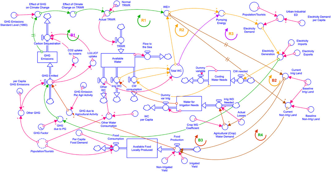
FIGURE 1. Stock-flow diagram for the national case study of Greece.

According to the Greek Statistical Authority (ELSTAT), Greece has a population of 10.4 million people (2020), which has been experiencing an ongoing decline since 2010 (Hellenic Statistical Authority, 2020). It is a popular touristic destination amassing over 30 million tourists per year, as was the case in 2019 (SETE, 2019). On the one hand, tourism is a significant factor for the Greek economy, and on the other hand, a demanding resource consumer, affecting resource availability and competing with antagonistic resource uses in the country. Furthermore, the agricultural sector in Greece has always been a reference point for economic and social life, thus contributing to 4% of the GDP, twice as much as in other European countries (Hellenic Statistical Authority, 2018), consuming close to 80% of all national freshwater resources and contributing to 7.84 million tons of GHG emissions (Our World in Data).

System Dynamics Model

System dynamics modeling has broadly been used as a simulator of complex real systems, helping researchers and policymakers to frame and understand the complexities of and interlinkages within the system, while at the same time, it provides information on how the system might evolve over time (Bakhshianlamouki et al., 2020). Τo conceptualize a complex dynamic system prior to simulation analysis, causal loop diagrams (CLDs) are used to identify the key variables in a system and indicate the causal relationship between them using links (Randers 1980). CLDs can perfectly describe the flow of the dynamic behavior of complex dynamic systems. A CLD consists of variables connected with links showing their interdependence and corresponding signs on each link that mark the nature of the paired connection—increase or decrease of the dependent variable; the number of increases or decreases defines the nature of the system behavior as a whole—making loops either reinforcing (multiplying the change in one direction) or balancing (breaking the chain, counterbalancing explosive system behavior, and resulting in reduced outcomes) (Lannon, 2012). Balancing or stabilizing feedback loops (Chapin et al., 2009) act by altering variables in the reverse direction to their existing one, neutralizing the effects of the condition on the system (Morecroft, 2015). Balancing the feedback loop is crucial because it can contribute to system recovery after a perturbation disappears. Reinforcing or amplifying feedback loops intensify the effects of the perturbations that contribute to destabilizing the system. The policies aiming at enhancing resilience might be used in “vicious” amplifying feedback loops by counterbalancing them to diminish or delay their effects on the outcome function of the system and mitigate the impact of perturbations. Whether loops are reinforcing or balancing, it depends on the number of negative relationships in a feedback loop: an even number of negative relationships indicates that the loop is positive (reinforcing), while an odd number indicates a negative (balancing) loop. Ideally, in each SDM, the existence of both, reinforcing and balancing loops, ensures the overall balance of the system.

As the next step, to quantify the variables in the loop, the stock-and-flow diagram (SFD) is used since SFDs can perfectly capture the stock and flow behavior of a system. Stocks are variables that represent accumulations (Richardson, 2011), and the flow is changing by decisions based on the condition of the system and can be simulated to generate the dynamic behavior of the system. Crucial stocks can enhance system resilience due to the by-default delay created between the disturbance and its effect. Thus, the system outcome function is less affected by the disturbance and saves time for easier recovery. The SFD represents integral finite difference equations involving the variables of the feedback loop structure of the system and simulates the dynamic behavior of the system (Manetsch and Park 1982; Bala et al., 2017).

The SDM (Figure 1) starts by simulating the GHG emissions as a stock, so GHGs in the atmosphere are the sum of what is emitted (GHG emitted) minus what is sequestrated (carbon sequestration). The GHG emitted is the sum of GHGs produced due to power generation (PG), GHGs due to agricultural activity, and other GHGs (i.e., urban/household) coming mainly from the population and tourists using the per capita GHG emissions (industrial GHG emissions are excluded from this calculation as they are deemed minor—see Laspidou et al., 2020). Carbon sequestration, on the other hand, depends on land use, land-use change, and forestry (LULUCF) uptake and CO₂ uptake by the oceans. As the GHG emissions change over time, the effect of GHGs on climate change varies accordingly, while the effect of climate change on total renewable water resources (TRWRs) is affected inversely; thus, an increase in GHG emissions leads to a decrease in the TRWR, reflecting the fact that climate change will bring about water scarcity in the long run. The TRWR is the inflow that feeds the available freshwater stock, while its outflows are: flow to the sea, (CW) consumption, the irrigation water consumption (WC), and other WC (household/urban WC). The sum of all these outflows (except from flow to the sea) is the total WC.

We use the Water Exploitation Index plus (WEI+) as a measurement of water stress in the country (Casadei et al., 2020). Values greater than 20% indicate water scarcity, while values greater than 40% indicate situations of severe water scarcity (i.e., the use of freshwater resources is clearly unsustainable) (EUROSTAT). WEI+ is affected by both actual TRWR and total WC. The former inversely affects the WEI+ (a delay signal has been used herein, indicating that changes in TRWR will become visible in the WEI+ in the long run), while the latter directly affects the WEI+. When the WEI + increases, it means that we have increasing deficits in freshwater availability, which leads to a drop in aquifer levels and an increase in pumping energy (PE) as we have to go deeper and deeper to find water. In turn, the electricity demand (ED) associated with pumping increases, followed by increased electricity generation to meet demands, which leads to both increased GHG emissions (when fossil fuels are used) and increased demands in CW, and thus in total WC, and a further increase in WEI+, creating a reinforcing loop (R3).

An increased WEI+, which is a result of either increased water consumption, decreased TRWR, or both, will in the long run result in farmers switching to alternative crops that do not require irrigation. This is a natural adaptation to climate change practice that farmers will follow. As a result, irrigated land and associated irrigation water demand will decrease and nonirrigated land should increase; this is not expected to be an immediate response to water scarcity; thus, a delay is taken into account in the SDM. Naturally, both irrigated and nonirrigated land affect food production (FP) and GHG emissions due to agricultural activity. Finally, all human consumption is represented and regulated by the population/tourist parameter directly affecting the following quantities in the model: urban–industrial ED, food consumption, other (urban) water consumption, and other (urban) GHG emissions. The CLDs formed in this SDM are presented in the Results section.

Sensitivity Analysis

With the purpose of developing confidence and validity in the model and its results, unit consistency and SA were implemented in the developed SDM; this analysis aims to prove that this model is sufficiently accurate for its intended use (Robinson, 2004). To check the unit consistency of our model, each model variable in the SDM was separately selected and either confirmed or amended to ensure that it is correct and in consistent units. In this combined nexus–resilience analysis, we used the SA to identify the most important parameters affecting the basic variables of the system by quantifying the importance of each parameter.

We start by performing sensitivity runs based on Monte Carlo simulations implemented in the SDM for all model parameters. The initial values of the parameters were altered by ±10% to observe the corresponding changes on the variables of the greatest interest in our model. We present the analysis for three important quantities, namely, available freshwater, ED, and GHG emissions. Our interest is to show how these quantities change when all parameters vary by ±10% with a Monte Carlo analysis. For some parameters, we observed almost no change, while for some others, we had significant variability. We show the results for a selected set of seven parameters that our quantities show variable sensitivity to. These are: TRWR (m³ of water), population/tourists (number), GHG emission factor for PG (kg of CO₂/GWh produced), per capita GHG emissions (kg of CO₂/capita due to human activity—mainly transportation), ED per capita (GWh electricity consumed/capita), irrigated land (m² of land), and actual losses in the agricultural irrigation system (m³ water). All data come from the SIM4NEXUS dataset (Mellios and Laspidou, 2020) and are expressed on a yearly basis.

To quantify sensitivity, we used Eq. 1, where $S\left(p\right)$ is the estimated sensitivity value of a parameter, x is the selected variable, p is the selected parameter, and $\mathrm{\Delta }x$ and $\mathrm{\Delta }p$ denote the change in the variable and parameter, respectively (Jørgensen and Bendoricchio, 2001). The larger the $S\left(p\right)$ value of a given parameter, the more important that parameter is.

$S\left(p\right)=\frac{\frac{\mathrm{\Delta }\mathit{x}}{\mathit{x}}}{\frac{\mathrm{\Delta }\mathit{p}}{\mathit{p}}},(1)$

System Resilience Analysis

In the context of implementing SRA, we investigated how our system responds to a disturbance $\left(\sigma \right)$. In our case study, we chose disturbance $\left(\sigma \right)$ to be the reduction of the TRWR (i.e., a drought) as a consequence of climate change. Our outcome function F(x) (i.e., available freshwater) indicates how the system responds to that disturbance. The purpose of this analysis is to investigate whether a system—after being affected by a disturbance $\left(\sigma \right)$—can recover or not and under which circumstances. More specifically, two things can happen to a system that has undergone shock or a very strong disturbance: it can either absorb the shock and result in maintaining its original behavior (no change) or it can change to a new state. When a system shifts to a new state, it can then either bounce back to its original state (a mechanical equivalent would be that the system “bends”) or be forced to a completely new permanent state and never bounce back to its original state (corresponding to the system “braking” according to our mechanical analogy) (Herrera de Leon and Kopainsky, 2019). When assessing system resilience, it is important to identify “when the disturbance forces the system to change its behavior”, or in other words, “how big a disturbance needs to be”, “under which circumstances and after how long the system bounces back or breaks”, and/or “how fast the system can recover”, if at all. To address the aforementioned questions, we follow the Herrera (2017) methodology and quantify system resilience by measuring five resilience metrics. To do this, we consider the available freshwater as the outcome function F(x) and quantify the system behavior after being affected by disturbance $\left(\sigma \right)$, which is an extreme drought, expressed as a steep reduction in the TRWR.

Engineering resilience and ecological resilience are both considered here. Engineering resilience is defined as the rate (how fast) at which a system resumes to its original state after a perturbation (Pimm 1984), whereas ecological resilience is defined as the amount of disturbance a system can withstand and not change into a new condition (Carpenter and Gunderson, 2001). As also described by Herrera (2017), for this analysis, we assess engineering resilience by using hardness, recover rapidity, and robustness measures, whereas to assess ecological resilience, we use elasticity and index of resilience measures. To define the aforementioned measures, we consider the following characteristics:$\delta$: magnitude of disturbance, $t_c$: time when the disturbance starts, $t_d$: time when the disturbance stops, and $t_f$: time when the system fully bounces back.

Hardness $\left({\sigma }_H\right)$ is the system’s ability to withstand a disturbance $\left(\sigma \right)$ without presenting a change in the performance of the outcome function $F\left(x\right)$. To measure hardness, we increase $\delta$ to find the smallest value of $\sigma$ that produces a different outcome function $F\left(x\right)$, while keeping $t_d$ and $t_c$ constant.

${\mathit{\sigma }}_{\mathit{H}}={\mathit{\delta }}_{\mathit{H}}\times \left(t_d-t_c\right).(2)$

Recover rapidity $\left(\overline{\mathit{R}}\right)$ is the average rate at which a system bounces back to its original situation after a disturbance $\left(\sigma \right)$ (Pimm, 1984; Martin et al., 2011; Herrera 2017). To measure $\overline{R}$, we continue increasing $\delta$, keeping $t_d$ and $t_c$ steady, and estimate the $F\left(t_{d_1}\right)$ for the current (original) situation and $F\left(t_{d_2}\right)$ after the disturbance $\left(\sigma \right)$:

$\left(\overline{\mathit{R}}\right)=\frac{\left(\mathit{F}\left({\mathit{t}}_{{\mathit{d}}_1}\right)-\mathit{F}\left({\mathit{t}}_{{\mathit{d}}_2}\right)\right)}{{\mathit{t}}_{\mathit{f}}-{\mathit{t}}_{\mathit{d}}}.(3)$

Robustness $\left(\overline{\mathit{\rho }}\right)$ is the system’s ability to resist big disturbances $\left(\sigma \right)$ without significant loss of performance (Attoh-Okine et al., 2009; Herrera 2017) and is given by Eq. 4:

$\left(\overline{\mathit{\rho }}\right)=\frac{\mathit{\sigma }}{\left(\mathit{F}\left({\mathit{t}}_{{\mathit{d}}_1}\right)-\mathit{F}\left({\mathit{t}}_{{\mathit{d}}_2}\right)\right)}.(4)$

Elasticity $\left({\mathit{\sigma }}_{\mathit{E}}\right)$ is the system’s ability to absorb a disturbance $\left(\sigma \right)$ without changing to a different permanent state (Holling, 1996; Herrera 2017). Elasticity is calculated as the smallest disturbance ${\sigma }_E$ that moves $F\left(x\right)$ to a different state. The bigger ${\sigma }_E$ a system has, the more undisturbed it is

${\mathit{\sigma }}_{\mathit{E}}={\mathit{\delta }}_{\mathit{E}}\times \left({\mathit{t}}_{\mathit{d}}-{\mathit{t}}_{\mathit{c}}\right).(5)$

Index of Resilience $\left({\mathit{I}}_{\mathit{res}}\right)$ is the probability of the system to keep its current situation steady (Holling, 1996; Holling and Gunderson, 2002; Martin et al., 2011). High values of $I_{res}$ indicate low probability of the system changing to a different state.

${\mathit{I}}_{res}=\mathit{P}\left(\mathit{\sigma }\le {\mathit{\sigma }}_{\mathit{E}}\right).(6)$

Results and Discussion

Causal Loop Diagrams

For this analysis, the conceptualization of the nexus system is presented through the construction of a CLD. The CLD (Figure 2) revealed seven interesting feedback loops–four reinforcing (R1, R2, R3, and R4) and three balancing ones (B1, B2, and B3). R1 is a climate–water–energy nexus reinforcing loop starting from the climate sector (Figure 3A). When the GHG produced due to PG is dealing with an increase, then the GHG emitted inflow is also increased, which in turn affects the GHG emissions the same way. An increase in GHG emissions causes a delayed increase on the effect of GHGs on climate change, while the effect of climate change on the TRWR is affected inversely, causing a decrease on the TRWR. When the TRWRs are reduced, WEI+—affected by TRWR—faces an increase which intensifies PE, ED, and EG, leading to a further increase in GHG produced due to PG. The R2 loop (Figure 3B) indicates the interconnection of total WC, WEI+, PE, ED, EG, and CW, where all are followed by successive increase, thus creating a water–energy nexus reinforcing loop. R3 in Figure 3C, is also a water–energy nexus reinforcing loop following the structure of R2, but in this loop, an increase in PE is caused by an increase in total WC due to the emerging need to extract more water to cover water demands (WEI+ is not part of this loop). In the R4 loop (Figure 3D), the GHG emissions affect the TRWR and WEI+ in the way described previously for R1. An increase in WEI + leads to a drop in water supply forcing the farmers to adapt to the new challenge by switching to nonirrigated crops, thus leading to an increase in nonirrigated land and FP. In turn, an increase in FP leads to a GHG emission increase through GHG due to agricultural activity, thus creating a reinforcing climate–water–food nexus loop.

FIGURE 2

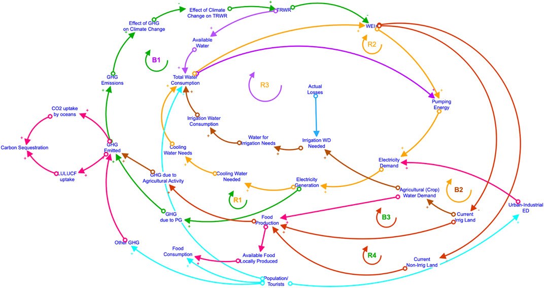
FIGURE 2. Causal loop diagram (CLD) indicating the interconnection of Greece’s water–energy–food system under climate change using the SDM.

FIGURE 3

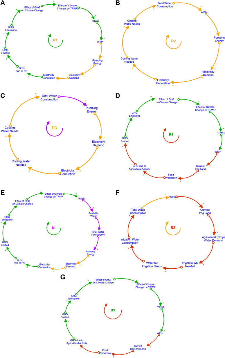
FIGURE 3. Individual causal loop diagrams (CLDs) indicating the four reinforcing and three balancing loops. (A) Water–energy–climate reinforcing loop, (B) water–energy reinforcing loop, (C) water–energy reinforcing loop, (D) water–food–climate reinforcing loop, (E) water–energy–climate balancing loop, (F) competitive water uses the balancing loop, and (G) water–food–climate balancing loop.

In the B1 loop (Figure 3E), an increase in GHG emissions causes a decrease in the TRWR through the effect of climate change on TRWR; thus, both water availability and WC are also decreased, meaning the energy sector is also facing a decrease contributing to less GHG emissions (through GHG due to PG). Balancing loop B1 contributes to the limitation of climate change effects on the water and energy sector, creating a climate–water–energy nexus loop. In the B2 loop (Figure 3F), an increase in total water consumption means that water scarcity is deteriorating, so the WEI + values increase. When the country faces water scarcity, farmers will adapt to this situation by limiting the cultivation of irrigating crops; thus, the irrigated land, the associated irrigation WD, and irrigation WC will decrease. This behavior sets limits to reckless water use and creates a competitive water use balancing loop. In the B3 loop (Figure 3G), similar to B2, an increase in WEI + causes a decrease in irrigated land, FP, and GHG emissions through the GHG emitted due to agricultural activity, thus creating a climate–water–food nexus balancing loop. The system comes to a relative balance due to the existence of both kinds of loops–reinforcing and balancing.

Following the model’s conceptualization, we then proceeded to the system’s SFD as depicted in Figure 1 to quantify the nexus interlinkages, find the most sensitive system parameters, and quantify system resilience for the three scenarios.

Sensitivity Analysis Results

Table 1 reveals the most important parameters that affect the whole system in a descending order based on parameter S(p) (Eq. 1). The TRWR and the number of people (population/tourists) seem to be the two parameters that our model is the most sensitive to, while the parameter actual losses in the irrigation network is the one that affects the model the least.

TABLE 1

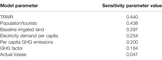
TABLE 1. Whole model’s parameter importance in descending order.

To quantify how much these seven model parameters affect the three basic quantities in the model, namely, available water, ED, and GHG emitted, we present a sector-specific SA, in which S(p) is calculated for each quantity, making it possible to compare and contrast the sensitivity of the important quantities to these parameters (Table 2). We observe that actual losses are at the bottom of the list, and the number of people (population/tourists) is close to the top of the list for all three quantities.

TABLE 2

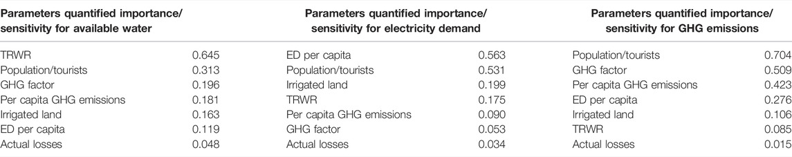
TABLE 2. Parameter quantified importance/sensitivity for available water, electricity demand, and GHG emissions in a descending order.

Next, a percentile analysis is performed. The most sensitive parameters are expected to bring about large variability in the quantities, while small variability indicates that the quantities do not change much, so they are insensitive to the parameters in question. Tornado diagrams are used to visually depict these results, showing the value of the quantity for the limiting values of the 5th and the 95th percentile of the parameter (Howard, 1988; Eschenbach, 1992). To show not only the limiting values but also the values of the quantities for the whole range of values that the parameter takes in the Monte Carlo analysis, we use sensitivity spread diagrams that were produced using the “ggplot2” plotting package in RStudio software. These results are shown in Figure 4. The climate sector is mostly affected by the population/tourists, GHG factor, and per capita GHG parameters (Figures 4A,B). The most important parameters of the water sector are TRWR and population/tourists (Figures 4C,D), while the energy sector is proved to be sensitive when ED per capita and population/tourists change (Figures 4E,F). Actual losses seem to affect these three sectors (and the whole system) the least.

FIGURE 4

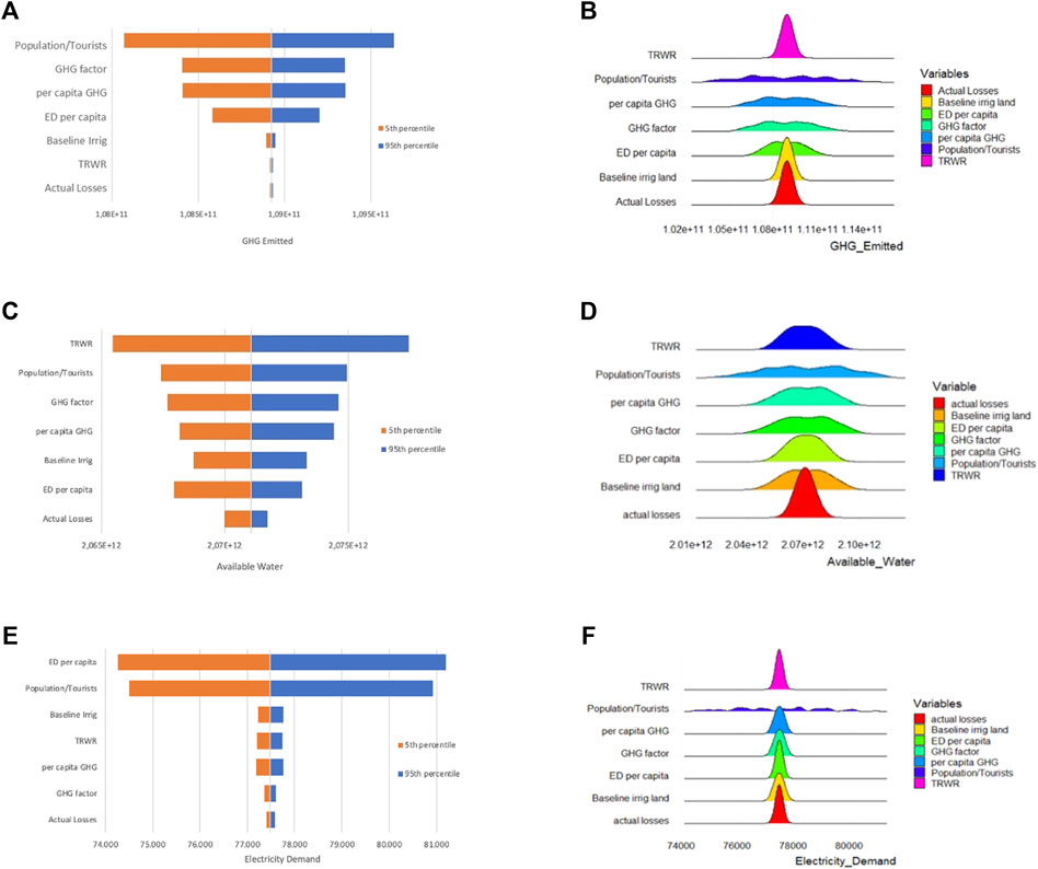
FIGURE 4. Tornado diagrams showing the value of the quantity for the limiting values of the 5th and the 95th percentile of the parameters for: (A) GHG emitted in kg CO₂, (C) available water in m3, and (E) electricity demand in GWh. Spread diagrams indicating values of the quantities for the whole range of values that the parameter takes in the Monte Carlo analysis for: (B) GHG Emitted in kg CO₂, (D) Available Water in m3, (F) Electricity Demand in GWh.

The spread diagrams indicate the values of the quantities for the whole range of values that the parameter takes in the Monte Carlo analysis for: b) GHG emitted in kg CO₂, d) available water in m3, and f) electricity demand in GWh.

To validate the results of the model, we used the WEI + values. We simulated the WEI + values starting from year 1 (corresponding to actual year 2010), and we compared the two values—simulated and real—for the year 7 (corresponding to actual year 2017). We chose the year 2017 since this is the last value published by EUROSTAT. The actual WEI + value for the year 2017 is 39.37% (European Environmental Agency (EEA), 2020), while the simulated value is 38.7%, thus validating model results.

Resilience Analysis and Policy Evaluation

To assess SRA for our case study, we study the system behavior and quantify its ability to withstand shock under climate change; in this case, an extreme drought scenario is imposed on the system, and its ability to withstand it is investigated. The ecological and engineering measures of resilience (system resilience analysis) were applied to the developed SDM for the baseline scenario (with no interventions) and also for two suggested policies aiming to enhance WEF security; the implementation of renewable energy systems (RESs) (policy I) and increased stakeholder awareness and education, followed by increased funding to implement advanced irrigation systems with minimal losses in agriculture (policy II).

In Figure 5, we show the SFD that includes the implementation of policy I. The outer loop shown with black arrows is reinforcing loop R1, while the balancing loop B1 combines black and blue arrows and goes through the available water stock and through total WC and pumping energy. For policy I, we add the parameter fraction of RES in total energy generation mix (shown in the box in Figure 5), and this way, we reduce the GHG emissions due to power generation by 30% as compared to the baseline scenario.

FIGURE 5

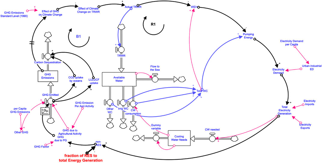
FIGURE 5. Stock-and-flow diagram with the implementation of policy I—renewable energy systems (RES).

For policy II, we add extra variables in the SDM, and a new loop is formed (reinforcing loop R5). Here, awareness and education is designed to lead to stakeholders demanding and obtaining more funding for the implementation of efficient irrigation technologies that will lead to increased irrigation efficiency and reduced actual losses in agriculture (Figure 6). We expect both policies to lead to more resilient water systems overall through a WEF analysis; our goal is to compare the two policies in terms of systemic resilience using the metrics presented in the system resilience analysis. Therefore, we simulate and measure the resilience function $F\left(x\right)$ (which represents the quantity of choice, depending on our scenario) for the baseline scenario (with no policies yet implemented); in our case, F(x) is available water. As the next step, the two proposed policies are applied separately to the system, and then the respective responses to the system are measured. “Before” and “after” results can then be compared to identify which scenario enhances the system resilience aiming at WEF security under climate change.

FIGURE 6

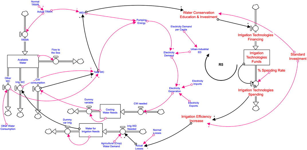
FIGURE 6. Stock-and-flow diagram with the implementation of policy II—funding to reduce water losses in irrigation systems.

We follow a methodology in order to define system hardness $\left({\sigma }_H\right)$ and elasticity $\left({\sigma }_E\right)$. To find system hardness, we keep increasing the magnitude of the system disturbance (TRWR reduction) over a period of 10 years, specifically from 2014 to 2024, and we observe how $F\left(x\right)$—available water—changes. The highest disturbance/change in the TRWR that produces the least noticeable change in $F\left(x\right)$ is its hardness $\left({\sigma }_H\right)$, the engineering threshold (shown in Table 3). We observe that when all scenarios are compared, the baseline is the least resilient system, having the lowest hardness, while policy I has the highest. With the implementation of policies, the system can withstand bigger changes (higher hardness) in the TRWR, such as extreme droughts caused by climate change, before available water is affected. Variable $\overline{R}$ shows how quickly the system will recover from the disturbance, and it is the highest for policy I, while in terms of robustness, the two policies appear similarly robust and more robust than the baseline. Ecological resilience is assessed next with the calculation of system elasticity $\left({\sigma }_E\right)$ and Index of Resilience $\left(I_{res}\right)$ for the same 10-year period (2014–2024). We now reduce the TRWR even more until the outcome $F\left(x\right)$—available water—changes significantly and to a new state, and we observe whether $F\left(x\right)$ bounces back or not. In a mechanical analog, we speak about the system “bending” and “not breaking”, that is, eventually recovering to its original state after some time. Again, policy I seems to perform the best, showing higher system elasticity and a significantly higher Index of Resilience overall. The system shows a higher overall resilience under policy I.

TABLE 3

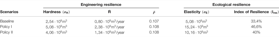
TABLE 3. Results of engineering and ecological resilience measures for the three scenarios; the baseline scenario, policy I—RES, and policy II—irrigation funding.

In Figure 7, we show graphically the function $F\left(x\right)$ for the three scenarios (baseline and policy I and II) along with the initial values (blue), hardness ${\sigma }_H$ (orange), and elasticity ${\sigma }_E$ (green). The initial values are improved for the two policies, with policy I being slightly better (curve slightly higher than the other blue curves). For hardness and elasticity, we need to compare the difference with the initial values. For hardness, we observe that the biggest difference is found between initial values and policy I, indicating that the system is the “hardest” with policy I. Policy II shows hardness that is improved from the baseline. For elasticity, again, policy I is the most “elastic” with the difference being significantly larger when comparing with policy II and baseline. This means that the system is more resilient, and even when there is a large perturbation, it is capable of “absorbing” it and bouncing back to its original state. When examining the baseline scenario, we observe that the system is capable of absorbing a small disturbance (indicated by hardness curve matching the initial value at 100 years), but it is not able to bounce back to its original state when a larger perturbation occurs. This is indicated when we observe that the green solid line (elasticity for baseline scenario) never meets the blue solid line (initial value, baseline scenario), but even 100 years later, it remains lower than the original curve. Thus, without the implementation of any policies, the system suffers a significant blow and never bounces back.

FIGURE 7

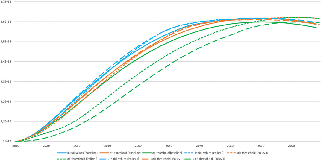
FIGURE 7. Simulated behavior for the available freshwater constituted of initial values of the TRWR (with no disturbance) and system thresholds of hardness and elasticity referring to the three scenarios: baseline scenario, policy I, and policy II.

Conclusion

New approaches on natural resource policymaking need to be applied with the intention to provide essential human needs and resources to all in an environmentally compatible, economically resilient, and socially inclusive manner that is capable of contending with perturbations. SES adaptation to climate change requires a more functional approach of resilience use in policymaking. System dynamic modeling prevails over other simulation techniques by supporting the analysis of system structure and focusing on feedback loop relationships. This study combines WEF nexus analysis under climate change with SA and SRA that are said to have the potential to deliver on these grand development challenges. The proposed methodology describes how to simulate the WEF nexus system under climate change for the national case study of Greece using system dynamic modeling, identify the most important (sensitive) system parameters, and quantify five essential metrics of resilient behavior (for three scenarios), thus providing the policymakers with a quantitative basis to enhance the resilience of SESs. Engineering ( ${\sigma }_H$, $\overline{R}$, and $\overline{\rho }$ ) and ecological ( ${\sigma }_{{\rm E}}$ and $I_{res}$ ) resilience measures are quantified, and the respective thresholds are also identified. In this study, two proposed policies are compared to decide which one enhances the system resilience best. Evaluating the results, we conclude that the Greek simulated system can withstand an extreme drought event affected for a 10-year period under the allowing circumstances of engineering and ecological thresholds found for the two policies (policy I and policy II); the baseline scenario has little tolerance to such disturbance (reduction on TRWR) and easily breaks when it overcomes the ecological threshold without being able to recover. Policy I proposing the implementation of RES seems to be the most promising scenario as its resilience measures have the highest values, so the system can even recover from the shock for a more severe drought, while policy II is also a good scenario since it contributes to system recovery when affected by drought although having lower resilience measures values by enhancing water security through irrigation funding techniques.

Data Availability Statement

Publicly available datasets were analyzed in this study. These data can be found here: https://data.mendeley.com/datasets/9x7wn24rrp/1.

Author Contributions

AI: conceptualization, methodology, software, validation, formal analysis, visualization, data curation, and writing—original draft preparation. CL: conceptualization, methodology, resources, writing—reviewing and editing, supervision, project administration, and funding acquisition.

Funding

The work described in this article has been conducted within the project NEXOGENESIS. This project has received funding from the European Union’s Horizon (2020) Research and Innovation Programme under Grant Agreement No. 1010003881 NEXOGENESIS. This article and the content included in it do not represent the opinion of the European Union, and the European Union is not responsible for any use that might be made of its content.

Conflict of Interest

The authors declare that the research was conducted in the absence of any commercial or financial relationships that could be construed as a potential conflict of interest.

Publisher’s Note

All claims expressed in this article are solely those of the authors and do not necessarily represent those of their affiliated organizations, or those of the publisher, the editors, and the reviewers. Any product that may be evaluated in this article, or claim that may be made by its manufacturer, is not guaranteed or endorsed by the publisher.

References

Albrecht, T. R., Crootof, A., and Scott, C. A. (2018). The Water-Energy-Food Nexus: A Systematic Review of Methods for Nexus Assessment. Environ. Res. Lett. 13, 043002. doi:10.1088/1748-9326/aaa9c6

CrossRef Full Text | Google Scholar

Allen, C. R., Angeler, D. G., Chaffin, B. C., Twidwell, D., and Garmestani, A. (2019). Resilience Reconciled. Nat. Sustain. 2 (10), 898–900. doi:10.1038/s41893-019-0401-4

PubMed Abstract | CrossRef Full Text | Google Scholar

Anderies, J. M. (2015). Managing Variance: Key Policy Challenges for the Anthropocene. Proc. Natl. Acad. Sci. U.S.A. 112 (47), 14402–14403. doi:10.1073/pnas.1519071112

PubMed Abstract | CrossRef Full Text | Google Scholar

Attoh-Okine, N. O., Cooper, A. T., and Mensah, S. A. (2009). Formulation of Resilience index of Urban Infrastructure Using Belief Functions. IEEE Syst. J. 3 (2), 147–153. doi:10.1109/jsyst.2009.2019148

CrossRef Full Text | Google Scholar

Bakhshianlamouki, E., Masia, S., Karimi, P., van der Zaag, P., and Sušnik, J. (2020). A System Dynamics Model to Quantify the Impacts of Restoration Measures on the Water-Energy-Food Nexus in the Urmia lake Basin, Iran. Sci. Total Environ. 708, 134874. doi:10.1016/j.scitotenv.2019.134874

PubMed Abstract | CrossRef Full Text | Google Scholar

Bala, B. K., Arshad, F. M., and Noh, K. M. (2017). “Systems Thinking: System Dynamics,” in System Dynamics (Singapore: Springer), 15–35. doi:10.1007/978-981-10-2045-2_2

CrossRef Full Text | Google Scholar

Bleischwitz, R., Spataru, C., VanDeveer, S. D., Obersteiner, M., van der Voet, E., Johnson, C., et al. (2018). Resource Nexus Perspectives towards the United Nations Sustainable Development Goals. Nat. Sustain. 1 (12), 737–743. doi:10.1038/s41893-018-0173-2

CrossRef Full Text | Google Scholar

Carpenter, S. R., and Gunderson, L. H. (2001). Coping with Collapse: Ecological and Social Dynamics in Ecosystem Management. BioScience 51 (6), 451–457. doi:10.1641/0006-3568(2001)051[0451:cwceas]2.0.co;2

CrossRef Full Text | Google Scholar

Casadei, S., Peppoloni, F., and Pierleoni, A. (2020). A New Approach to Calculate the Water Exploitation Index (WEI+). Water 12 (11), 3227. doi:10.3390/w12113227

CrossRef Full Text | Google Scholar

F. S. ChapinIII, G. P. Kofinas, and C. Folke (Editors) (2009). Principles of Ecosystem Stewardship: Resilience-Based Natural Resource Management in a Changing World (Springer Science & Business Media).

Google Scholar

Chen, X., Wang, D., Tian, F., and Sivapalan, M. (2016). From Channelization to Restoration: Sociohydrologic Modeling with Changing Community Preferences in the Kissimmee River Basin, Florida. Water Resour. Res. 52 (2), 1227–1244. doi:10.1002/2015WR018194

CrossRef Full Text | Google Scholar

Coyle, R. G. (1997). System Dynamics Modelling: A Practical Approach. J. Oper. Res. Soc. 48 (5), 544.

CrossRef Full Text | Google Scholar

C. S. Holling, and L. H. Gunderson (Editors) (2002). Panarchy: Understanding Transformations in Human and Natural Systems (Washington, DC: Island Press).

Google Scholar

De Grenade, R., House-Peters, L., Scott, C., Thapa, B., Mills-Novoa, M., Gerlak, A., et al. (2016). The Nexus: Reconsidering Environmental Security and Adaptive Capacity. Curr. Opin. Environ. sustainability 21, 15–21. doi:10.1016/j.cosust.2016.10.009

CrossRef Full Text | Google Scholar

Eschenbach, T. G. (1992). Spiderplots versus Tornado Diagrams for Sensitivity Analysis. Interfaces 22 (6), 40–46. doi:10.1287/inte.22.6.40

CrossRef Full Text | Google Scholar

European Environmental Agency (EEA) (2020). Development of the Water Exploitation index Plus (WEI+). Copenhagen. Available from: https://www.eea.europa.eu/data-and-maps/daviz/water-exploitation-index-plus#tab-chart_1_filters=%7B%22rowFilters%22%3A%7B%7D%3B%22columnFilters%22%3A%7B%22pre_config_year%22%3A%5B%222017%22%5D%7D%3B%22sortFilter%22%3A%5B%22wei_2017_reversed%22%5D%7D (Accessed November 8, 2021).

Google Scholar

European Union’s Horizon (2020). European Union’s Horizon. Available from: https://ec.europa.eu/info/research-and-innovation/funding/funding-opportunities/funding-programmes-and-open-calls/horizon-2020_en.

Google Scholar

Finley, J. W., and Seiber, J. N. (2014). The Nexus of Food, Energy, and Water. J. Agric. Food Chem. 62 (27), 6255–6262. doi:10.1021/jf501496r

PubMed Abstract | CrossRef Full Text | Google Scholar

Flammini, A., Puri, M., Pluschke, L., and Dubois, O. (2014). Walking the Nexus Talk: Assessing the Water-Energy-Food Nexus in the Context of the Sustainable Energy for All Initiative. Rome: Fao.

Google Scholar

Folke, C., Carpenter, S. R., Walker, B., Scheffer, M., Chapin, T., and Rockström, J. (2010). Resilience Thinking: Integrating Resilience, Adaptability and Transformability. Ecol. Soc. 15 (4), 150420. doi:10.5751/es-03610-150420

CrossRef Full Text | Google Scholar

Ford, A. (1999). Modelling the Environment. An Introduction to System Dynamics Modelling of Environmental Systems. Washington, D.C: Island Press, 401.

Google Scholar

Forrester, J. W. (1961). Industrial Dynamics. Cambridge, MA: MIT Press.

Google Scholar

Grafton, R. Q., McLindin, M., Hussey, K., Wyrwoll, P., Wichelns, D., Ringler, C., et al. (2016). Responding to Global Challenges in Food, Energy, Environment and Water: Risks and Options Assessment for Decision-Making. Asia Pac. Pol. Stud. 3 (2), 275–299. doi:10.1002/app5.128

CrossRef Full Text | Google Scholar

Grafton, R. Q., Doyen, L., Béné, C., Borgomeo, E., Brooks, K., Chu, L., et al. (2019). Realizing Resilience for Decision-Making. Nat. Sustain. 2, 907–913. doi:10.1038/s41893-019-0376-1

CrossRef Full Text | Google Scholar

Guillaume, J., Kummu, M., Eisner, S., and Varis, O. (2015). Transferable Principles for Managing the Nexus: Lessons from Historical Global Water Modelling of Central Asia. Water 7, 4200–4231. doi:10.3390/w7084200

CrossRef Full Text | Google Scholar

Hall, J. W., Grey, D., Garrick, D., Fung, F., Brown, C., Dadson, S. J., et al. (2014). Coping with the Curse of Freshwater Variability. Science 346, 429–430. doi:10.1126/science.1257890

PubMed Abstract | CrossRef Full Text | Google Scholar

Hellenic Statistical Authority (2018). Water Use (2000 - 2018). Piraeus, Greece. (Accessed November 8, 2021).

Google Scholar

Hellenic Statistical Authority (2020). Estimated Population and Migration Flows. Piraeus, Greece. Available from: https://www.statistics.gr/en/statistics/-/publication/SPO18/ (Accessed November 8, 2021).

Google Scholar

Herrera de Leon, H. J., and Kopainsky, B. (2019). Do you bend or Break? System Dynamics in Resilience Planning for Food Security. Syst. Dyn. Rev. 35 (4), 287–309. doi:10.1002/sdr.1643

CrossRef Full Text | Google Scholar

Herrera, H. (2017). From Metaphor to Practice: Operationalizing the Analysis of Resilience Using System Dynamics Modelling. Syst. Res. 34 (4), 444–462. doi:10.1002/sres.2468

CrossRef Full Text | Google Scholar

Hoekstra, A. Y., and Wiedmann, T. O. (2014). Humanity's Unsustainable Environmental Footprint. Science 344, 1114–1117. doi:10.1126/science.1248365

PubMed Abstract | CrossRef Full Text | Google Scholar

Hoff, H. (2011). Understanding the Nexus. Background Paper for the Bonn 2011 Nexus Conference: The Water, Energy and Food Security Nexus. Stockholm: Stockholm Environment Institute.

Google Scholar

Howard, R. A. (1988). Decision Analysis: Practice and Promise. Manag. Sci. 34 (6), 679–695. doi:10.1287/mnsc.34.6.679

CrossRef Full Text | Google Scholar

Holling, C. S. (1973). Resilience and Stability of Ecological Systems. Annu. Rev. Ecol. Syst. 4, 1–23. doi:10.1146/annurev.es.04.110173.000245

CrossRef Full Text | Google Scholar

Holling, C. S. (1996). Engineering within Ecological Constraints. Eng. within Ecol. constraints 31, 32. doi:10.17226/4919

CrossRef Full Text | Google Scholar

International Energy Agency (2010). World Energy Outlook. Retrieved from: http://sdg.iisd.org/news/iea-releases-world-energy-outlook-2010/811 (Accessed November 8, 2021).

Google Scholar

Ioannou, A. E., and Laspidou, C. S. (2018). “The Water-Energy Nexus at City Level: The Case Study of Skiathos,”. Multidisciplinary Digital (Lefkada, Greece: Publishing Institute Proceedings), 2, 694. doi:10.3390/proceedings2110694No. 11

CrossRef Full Text | Google Scholar

Janssen, D. N. G., Ramos, E. P., Linderhof, V., Polman, N., Laspidou, C., Fokkinga, D., et al. (2020). The Climate, Land, Energy, Water and Food Nexus Challenge in a Land Scarce Country: Innovations in the Netherlands. Sustainability 12 (24), 10491. doi:10.3390/su122410491

CrossRef Full Text | Google Scholar

Jørgensen, S. E., and Bendoricchio, G. (2001). Fundamentals of Ecological Modelling, 21. Elsevier.

Google Scholar

Kelly, R. A., Jakeman, A. J., Barreteau, O., Borsuk, M. E., ElSawah, S., Hamilton, S. H., et al. (2013). Selecting Among Five Common Modelling Approaches for Integrated Environmental Assessment and Management. Environ. Model. Softw. 47, 159–181. doi:10.1016/j.envsoft.2013.05.005

CrossRef Full Text | Google Scholar

Kitamori, K., Manders, T., Dellink, R., and Tabeau, A. A. (2012). OECD Environmental Outlook to 2050: The Consequences of Inaction. Paris: OECD.

Google Scholar

Lannon, C. (2012). Causal Loop Construction: the Basics. Syst. Thinker 23 (8), 7–8.

Google Scholar

Laspidou, C., Mellios, N., and Kofinas, D. (2019). Towards Ranking the Water-Energy-Food-Land Use-Climate Nexus Interlinkages for Building a Nexus Conceptual Model with a Heuristic Algorithm. Water 11 (2), 306. doi:10.3390/w11020306

CrossRef Full Text | Google Scholar

Laspidou, C. S., Mellios, N. K., Spyropoulou, A. E., Kofinas, D. T., and Papadopoulou, M. P. (2020). Systems Thinking on the Resource Nexus: Modeling and Visualisation Tools to Identify Critical Interlinkages for Resilient and Sustainable Societies and Institutions. Sci. Total Environ. 717, 137264. doi:10.1016/j.scitotenv.2020.137264

PubMed Abstract | CrossRef Full Text | Google Scholar

Leck, H., Conway, D., Bradshaw, M., and Rees, J. (2015). Tracing the Water-Energy-Food Nexus: Description, Theory and Practice. Geogr. Compass 9, 445–460. doi:10.1111/gec3.12222

CrossRef Full Text | Google Scholar

Malagó, A., Comero, S., Bouraoui, F., Kazezyılmaz-Alhan, C. M., Gawlik, B. M., Easton, P., et al. (2021). An Analytical Framework to Assess SDG Targets within the Context of WEFE Nexus in the Mediterranean Region. Resour. Conservation Recycling 164, 105205. doi:10.1016/j.resconrec.2020.105205

CrossRef Full Text | Google Scholar

Manetsch, T. J., and Park, G. L. (1982). System Analysis and Simulation with Applications to Economic and Social Systems. Michigan: Department of Electrical Engineering and System Science, Michigan State University.

Google Scholar

Martin, S., Deffuant, G., and Calabrese, J. M. (2011). “Defining Resilience Mathematically: from Attractors to Viability,”. Viability and Resilience ofComplex Systems. Editors G. Deffuant, and N. Gilbert (Berlin: Springer), 4, 15–36. doi:10.1007/978-3-642-20423-4_2

CrossRef Full Text | Google Scholar

Mellios, N., and Laspidou, C. (2020). “Water-Energy-Food-Land-Climate Nexus Data for the Case Study of Greece: National and River Basin District Scale”. London, United Kingdom: Mendeley Data, V1, doi:10.17632/9x7wn24rrp.1

CrossRef Full Text | Google Scholar

Mguni, P., and van Vliet, B. J. (2020). Rethinking the Urban Nexus-Resilience and Vulnerability at the Urban Nexus of Water, Energy and Food (WEF). An Introduction to the Special Issue. J. Integr. Environ. Sci. 17, 617. doi:10.1080/1943815X.2020.1866617

CrossRef Full Text | Google Scholar

Morecroft, J. D. (2015). Strategic Modelling and Business Dynamics: A Feedback Systems Approach. New York: John Wiley & Sons

Mpandeli, S., Naidoo, D., Mabhaudhi, T., Nhemachena, C., Nhamo, L., Liphadzi, S., et al. (2018). Climate Change Adaptation through the Water-Energy-Food Nexus in Southern Africa. Int. J. Environ. Res. Public Health 15 (10), 2306. doi:10.3390/ijerph15102306

PubMed Abstract | CrossRef Full Text | Google Scholar

Nyström, M., Jouffray, J.-B., Norström, A. V., Crona, B., Søgaard Jørgensen, P., Carpenter, S. R., et al. (2019). Anatomy and Resilience of the Global Production Ecosystem. Nature 575, 98–108. doi:10.1038/s41586-019-1712-3

PubMed Abstract | CrossRef Full Text | Google Scholar

Papadopoulou, C.-A., Papadopoulou, M., Laspidou, C., Munaretto, S., and Brouwer, F. (2020). Towards a Low-Carbon Economy: a Nexus-Oriented Policy Coherence Analysis in Greece. Sustainability 12 (1), 373. doi:10.3390/su12010373

CrossRef Full Text | Google Scholar

Pimm, S. L. (1984). The Complexity and Stability of Ecosystems. Nature 307, 321–326. doi:10.1038/307321a0

CrossRef Full Text | Google Scholar

Puma, M. J. (2019). Resilience of the Global Food System. Nat. Sustain. 2, 260–261. doi:10.1038/s41893-019-0274-6

CrossRef Full Text | Google Scholar

Randers, J. (1980). Guidelines for Model Conceptualization. Elem. Syst. Dyn. method 117, 139.

Google Scholar

Richardson, G. P. (2011). Reflections on the Foundations of System Dynamics. Syst. Dyn. Rev. 27 (3), 219–243.

CrossRef Full Text | Google Scholar

Robinson, C. (1998). Dynamical Systems: Stability, Symbolic Dynamics, and Chaos. Boca Raton, FL: CRC Press.

Google Scholar

Robinson, S. (2004). Simulation: The Practice of Model Development and Use, 1. Inglaterra: John Willey and Sons. Inc. Cap, 5.2

Google Scholar

Sachs, J. D., Schmidt-Traub, G., Mazzucato, M., Messner, D., Nakicenovic, N., and Rockström, J. (2019). Six Transformations to Achieve the Sustainable Development Goals. Nat. Sustain. 2, 805–814. doi:10.1038/s41893-019-0352-9

CrossRef Full Text | Google Scholar

Scheffer, M., Carpenter, S. R., Lenton, T. M., Bascompte, J., Brock, W., Dakos, V., et al. (2012). Anticipating Critical Transitions. Science 338, 344–348. doi:10.1126/science.12252410.1126/science.1225244

PubMed Abstract | CrossRef Full Text | Google Scholar

Scott, C. A., Pierce, S. A., Pasqualetti, M. J., Jones, A. L., Montz, B. E., and Hoover, J. H. (2011). Policy and Institutional Dimensions of the Water-Energy Nexus. Energy Policy 39, 6622–6630. doi:10.1016/j.enpol.2011.08.013

CrossRef Full Text | Google Scholar

SETE (2019). Basic Sizes of Greek Tourism. Available from: https://sete.gr/el/stratigiki-gia-ton-tourismo/vasika-megethi-tou-ellinikoy-tourismoy/ (Accessed November 8, 2021).

Google Scholar

Steffen, W., Rockström, J., Richardson, K., Lenton, T. M., Folke, C., Liverman, D., et al. (2018). Trajectories of the Earth System in the Anthropocene. Proc. Natl. Acad. Sci. U.S.A. 115 (33), 8252–8259. Proc. doi:10.1073/pnas.1810141115

PubMed Abstract | CrossRef Full Text | Google Scholar

Stephan, R. M., Mohtar, R. H., Daher, B., Embid Irujo, A., Hillers, A., Ganter, J. C., et al. (2018). Water-energy-food Nexus: a Platform for Implementing the Sustainable Development Goals. Water Int. 43 (3), 472–479. doi:10.1080/02508060.2018.1446581

CrossRef Full Text | Google Scholar

Stringer, L. C., Quinn, C. H., Le, H. T. V., Msuya, F., Pezzuti, J., Dallimer, M., et al. (2018). A New Framework to Enable Equitable Outcomes: Resilience and Nexus Approaches Combined. Earth's Future 6, 902–918. doi:10.1029/2017ef000694

CrossRef Full Text | Google Scholar

Sukhwani, V., Shaw, R., Mitra, B. K., and Yan, W. (2019). Optimizing Food-Energy-Water (FEW) Nexus to foster Collective Resilience in Urban-Rural Systems. Prog. Disaster Sci. 1, 100005. doi:10.1016/j.pdisas.2019.100005

CrossRef Full Text | Google Scholar

Turner, B. L., Kasperson, R. E., Matson, P. A., McCarthy, J. J., Corell, R. W., Christensen, L., et al. (2003). A Framework for Vulnerability Analysis in Sustainability Science. Proc. Natl. Acad. Sci. U.S.A. 100, 8074–8079. doi:10.1073/pnas.1231335100

PubMed Abstract | CrossRef Full Text | Google Scholar

UNDP (2016). Human Development Report 2016—human Development Foreveryone. New York, NY: United Nations Development Programme.

Google Scholar

UNFCCC (2011). Compilation of Information on Nationally Appropriate Mitigation Actions to Be Implemented by Parties Not Included in Annex I to the Convention. Bonn, Germany: United Nations Framework Convention on Climate Change. Available from: http://unfccc.int/resource/docs/2011/awglca14/eng/inf01.pdf.

Google Scholar

van Emmerik, T. H. M., Li, Z., Sivapalan, M., Pande, S., Kandasamy, J., Savenije, H. H. G., et al. (2014). Socio-hydrologic Modeling to Understand and Mediate the Competition for Water between Agriculture Development and Environmental Health: Murrumbidgee River basin, Australia. Hydrol. Earth Syst. Sci. 18 (10), 4239–4259. doi:10.5194/hess-18-4239-2014

CrossRef Full Text | Google Scholar

Vörösmarty, C. J., McIntyre, P. B., Gessner, M. O., Dudgeon, D., Prusevich, A., Green, P., et al. (2010). Global Threats to Human Water Security and River Biodiversity. Nature 467, 555–561. doi:10.1038/nature09440

PubMed Abstract | CrossRef Full Text | Google Scholar

Walker, B., Gunderson, L. H., Knizig, A., Folke, C., and Carpenter, S. (2006). A Handful of Heuristics and Some Propositions for Understanding Resilience in Social-Ecological Systems. Ecol. Soc. 11 (1), 13. doi:10.5751/es-01530-110113

CrossRef Full Text | Google Scholar

WEF (2011). Water Security: The Water–Food–Energy–Climate Nexus. Washington DC: World Economic Forum.

Google Scholar

World Bank (2013). World Development Report 2014: Risk and Opportunity—Managing Risk for Development. Washington, DC: World Bank.

Google Scholar